Chapter 6 Biscuit model validation 6.1

(1)

Chapter 6

Biscuit model validation

6.1 Introduction

In the previous chapters the physical model and the equations necessary to write a baking model were described. Moreover, in chapter 5 all the parameters necessary were found thanks to rheological characterization. In order to validate and extend the model, the validation tests were conducted on flour 1, which is the standard flour used in the UB baking process, and then, to see how the model was capable of following changes in the working conditions, the effects of both the recipes and rheology were studied. The results are reported only as simulations while for the other rheology some experimental data of another flour, called flour 2, were available, thus a comparison was also possible. To have good model results, sensitivity tests on the baking model are very important together with changing some initial values, like the void fraction, to test the capability of the program to predict the final biscuits properties, in agreement with industrial experience.

The model computation gives the values of the variables considered in the model at any instant and at any position and comparison was made by using the data obtained from UB by means of the so-called Brandstorm.

6.2 Heat fluxes and program graphic interface

Two different heat fluxes were considered to test the model sensitivity. The considered fluxes are industrial standard for baking and give different final texture and height due to the heating rate. The thermal history for the biscuit baking can be “fast” and “slow”: in this way in this chapter two different thermal profiles called K2 and STD are considered, which are fast and slow respectively. The model input was given in terms of measured heat flux, and the two different profiles, K2 and STD, were considered and reported in Fig.6.1 and Fig.6.2 respectively. A suitable fitting data software (Cubic Spline) was used to obtain the needed equations by interpolation, which in turn are used as boundary conditions.

(2)

K2 Spline 0 2000 4000 6000 8000 10000 12000 14000 0 50 100 150 200 250 time, s G, W/m^2 GTop real GBottom real GTop simul GBottom simul GTop GBottom

Figure 6. 1 – Cubic spline for K2 profile Std Fitting 0 1000 2000 3000 4000 5000 6000 7000 8000 0 50 100 150 200 250 300 time, s G, W/m^2 GTop real GBottom real GTop simul GBottom simul GTopGTo GBottom GBottom

(3)

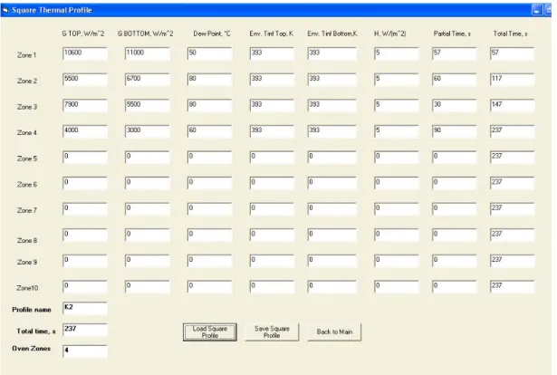
The predictive model of the final biscuit properties was implemented with a user friendly interface to allow the rheological properties, initial conditions and geometry, convection coefficient and the bulk temperature, heat fluxes and humidity bulk profiles to be changed. The interface, shown in figure 6.3, allows all the parameters to be loaded and permits a choice between spline heat fluxes (“fitted oven profile” button) and square fluxes. In the case of the latter option, the baking period is divided into definite zones in which the fluxes and humidity bulk value are constant (figure 6.4).

(4)

Figure 6. 4 – Interface to load square profiles

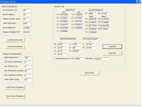
All the parameters can be loaded in the form shown in figure 6.5. As can be seen, the form is divided into three parts: geometrical, initial conditions and rheological.

It is possible to modify, save and upload the stored configuration. Moreover, the process parameters can be changed: initial temperature, tray surface void fraction, tray thickness, water content and R.A amount.

Finally, it is possible to change the flour when its rheological behaviour is known. In fact, the dough properties may be inserted, modified and stored.

Data of top and bottom heat flux and dew point can be uploaded from the files. Data will be fitted automatically by applying a cubic spline method and in real time shown in the form. Then, it is possible to upload data independently.

(5)

Figure 6. 5 – Process set up form

(6)

With these presuppositions, it is possible to simulate a specific biscuit baking and, when the simulation is completed, the main output (biscuit height, water content, surface and core temperature) are shown in the graph. Finally all the data obtained from the program can be downloaded onto an excel sheet.

Figure 6. 7 – Principal program outputs

To tests the model capability of predicting the final characteristics of the biscuit and the thermal profile of the sample, many simulations were carried out with this model that are reported later on.

6.3 Simulations for standard flour

The simulation results with flour 1 are shown in the following pictures and are reported in terms of temperature patterns in three different biscuit positions for the two different baking profiles and height profile stated in the previous chapter.

(7)

Temperature Profile (K2) 300 320 340 360 380 400 420 440 460 480 0 50 100 150 200 250 Time, s T, K

Simul_Bottom Real_Bottom Simul_Top

Real_Top Simul_Core Real_Core

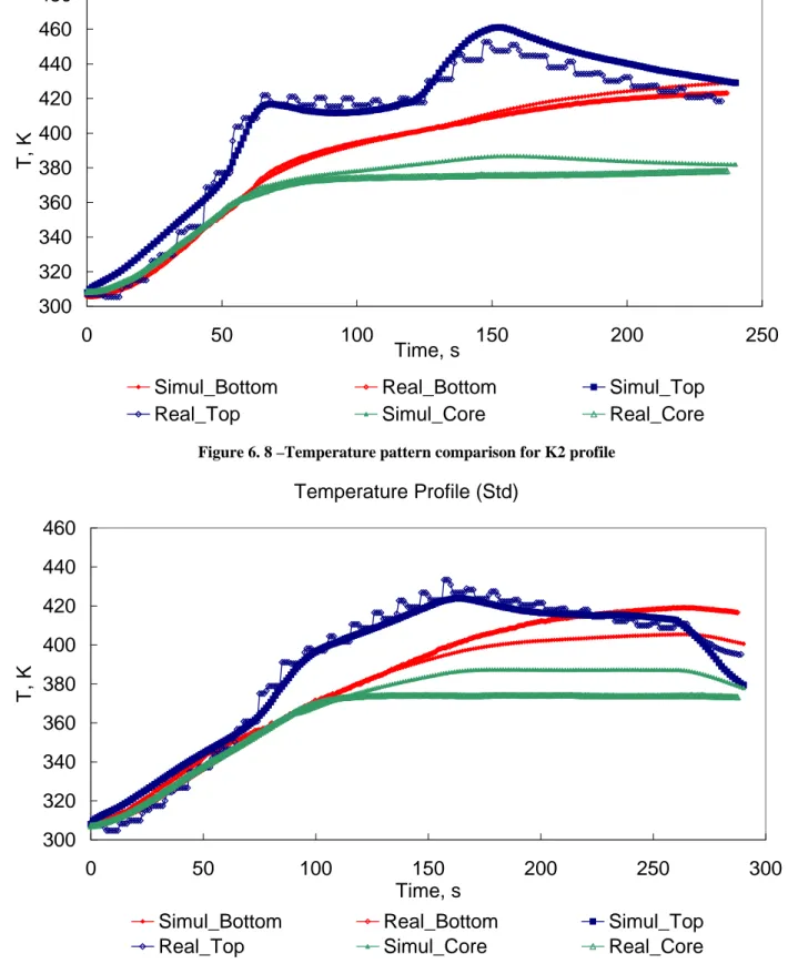
Figure 6. 8 –Temperature pattern comparison for K2 profile Temperature Profile (Std) 300 320 340 360 380 400 420 440 460 0 50 100 150 200 250 300 Time, s T, K

(8)

A good agreement between the model predictions and experimental data was found at any position of the system for the considered flux input, therefore denoting a good sensitivity of the proposed model to follow different fluxes (figure 6.8 and 6.9). The results give also an idea of the goodness of the temperature computation and in turn of the energy balance.

The simulation of the transient height of the biscuit is shown in Figure 6.10 for the considered case. A rather good agreement for both the oven profiles was found for the initial slope, the time at which collapse starts and the shape of the curve after collapse. The following height decrease is sufficiently acceptable for the STD profile and is in very good agreement for K2.

Height Profile 2 3 4 5 6 7 8 9 0 50 100 150 200 250 300 Time, s Heig ht, mm

K2_Simul K2_Real Std_Simul Std_Real

Figure 6. 10 – Simulated and experimental biscuit height

To show the observed differences the weight loss is reported in figure 6.11 where the above findings are enhanced. The agreement is not excellent, but the trend is the right one and the time at which the weight starts to decrease is sufficiently fitted. In every case, the difference between the real and the simulated profile is in the range of 5% error.

(9)

Weight Loss Profile 8 8.5 9 9.5 10 10.5 0 50 100 150 200 250 300 Time, s We igh t, g

K2_Real K2_Simul Std_Real Std_Simul Figure 6. 11 – Simulated and experimental weight loss

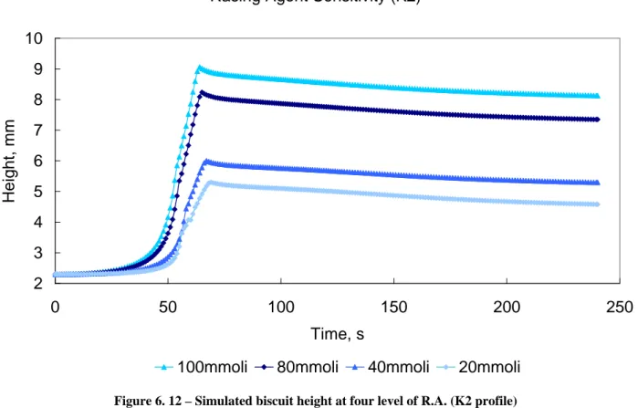
Then to verify the capability of the proposed model to follow parameter changes, four levels of raising agent (R.A.) initial concentration were studied. The comparison is made with a level of 80 mmole/kg dough of R.A., which is the standard industrial value used during baking. In figure 6.12 and 6.13 are reported the height profiles when changing the R.A. level. The dependence on the R.A. concentration is not proportional as a consequence of the mixing and standing process steps, during which some gas is lost. The values and the general shape are in agreement with practical experience, in particular the STD and K2 profiles are in the right order, the former being lower and shifted towards a higher time with respect to the latter. In figures 6.14 and 6.15 the computed temperature profile at the surface are reported and the results are in good agreement with expectations. In fact, when the level of R.A. is greater, it is normal to expect a higher final height with respect to lower R.A. concentrations and as a consequence a higher final void fraction. As a matter of fact, the literature data indicates that adding R.A., the consistency of the material decreases, allowing the bubbles present inside the dough to expand more easily. As a consequence the surface temperature increase being a function of the degree of void, and specifically by increasing the ε factor, conductivity decreases, causing a higher surface temperature.

(10)

Rasing Agent Sensitivity (K2) 2 3 4 5 6 7 8 9 10 0 50 100 150 200 250 Time, s Heig ht, mm

100mmoli 80mmoli 40mmoli 20mmoli

Figure 6. 12 – Simulated biscuit height at four level of R.A. (K2 profile) Rasing Agent Sensitivity (Std)

2 2.5 3 3.5 4 4.5 5 5.5 6 6.5 7 0 50 100 150 200 250 300 Time, s Heig ht, mm

(11)

Temperature Profiles @ Different Rasing Agent (K2) 300 320 340 360 380 400 420 440 460 480 500 0 50 100 150 200 250 Time, s T, K

Figure 6. 14 – Temperature profiles at four R. A. level (K2) Temperature Profiles @ Different Rasing Agent (Std)

300 320 340 360 380 400 420 440 460 0 50 100 150 200 250 300 Time, s T, K

(12)

The weight loss is also computed and the results for the two oven profiles are shown in the following figures.

Weight Loss Profiles @ Different Rasing Agent (K2)

8 8.4 8.8 9.2 9.6 10 0 50 100 150 200 250 Time, s W e ight , g

Figure 6. 16 – Simulated weight loss at four R.A. levels (K2). Weight Loss Profiles @ Different Rasing Agent (Std)

8 8.4 8.8 9.2 9.6 10 0 50 100 150 200 250 300 Time, s W e ight , g

(13)

Three values of void fraction were chosen close to the actual value and simulations were performed, the results are reported in terms of biscuit height (figures 6.18-6.19), surface temperature (figures 6.20-6.21) of biscuit and weight loss in figures 6.22-6.23 as already done above for both the considered oven profiles. It appears clearly that the larger the void fraction the lower the collapse as a consequence of the lower elastic energy stored. This was expected by the technician and the weight loss does not show any significant difference in both cases.

Void Fraction Sensitivity (K2)

2 3 4 5 6 7 8 9 0 50 100 150 200 250 Time, s H e ight, mm

Eps 0.05 Eps 0.04 Eps 0.03

(14)

Void Fraction Sensitivity (Std) 2 3 4 5 6 7 0 50 100 150 200 250 300 Time, s H e ight, mm

Eps 0.05 Eps 0.04 Eps 0.03

Figure 6. 19 - Simulated biscuit height at three void fraction (STD)

Temperature Profiles @ Different Void Fraction (K2)

300 320 340 360 380 400 420 440 460 480 500 0 50 100 150 200 250 Time, s T, K

Eps 0.05 Eps 0.04 Eps 0.03

(15)

Temperature Profiles @ Different Void Fraction (Std) 300 320 340 360 380 400 420 440 0 50 100 150 200 250 300 Time, s T, K

Eps 0.05 Eps 0.04 Eps 0.03

Figure 6. 21 - Simulated temperature profiles at three void fraction (STD)

Weight Loss Profiles @ Different Void Fraction (K2)

8 8.5 9 9.5 10 0 50 100 150 200 250 Time, s Weight,g

Eps 0.05 Eps 0.04 Eps 0.03

(16)

Weight Loss Profiles @ Different Void Fraction (Std) 8 8.5 9 9.5 10 0 50 100 150 200 250 300 Time, s We igh t, g

Eps 0.05 Eps 0.04 Eps 0.03

Figure 6. 23 - Simulated weight loss profiles at three void fraction (STD)

6.4 Rheological model sensitivity.

A different flour type was used to see the effect of rheology change,. Then, using the data available from rheological characterization, the computations were performed. A good agreement for the surface temperature was found only for the STD oven conditions, while it looks rather poor for the K2, but observing the profiles very well it can be noticed that the difference between simulated and real profile is in the range of 5%.

Of course, also the height reported in figure 6.26 suffers from the temperature differences observed. However, it can also be considered that the simulations are coherent even if the height is less and then the collapse behaviour is rather interesting, that has a well-predicted percentage. It is conviction that the difference between the real and simulated profiles depend on the uncertainty in the “Rupture work “ experimental data, affected by experimental error (see chapter V) of about 18%, while flour 1 has a parameter with 9.7% of error. In fact, adding the maximum standard deviation at the “rupture work” parameter, the profiles clearly improves (figure 6.28).

(17)

In figure 6.27 the weight loss is reported and as can be seen from the figure the weight loss for the standard profile is in very good agreement with the real trend and the final moisture value.

Temperature Profile (K2) 300 320 340 360 380 400 420 440 460 0 50 100 150 200 250 Time, s T, K

(18)

Temperature Profile (Std) 300 320 340 360 380 400 420 440 0 50 100 150 200 250 300 Time, s T, K

Figure 6. 25 - Simulated temperature profiles for flour 2 (STD) Height Profile 2 3 4 5 6 7 8 9 0 50 100 150 200 250 300 Time, s Heig ht, mm

(19)

Weight Loss Profile 8 8.5 9 9.5 10 10.5 0 50 100 150 200 250 300 Time, s We igh t, g

K2_Real K2_Simul Std_Real Std_Simul

Figure 6. 27 - Simulated weight loss profiles for flour 2 STD and K2 Height Profile 2 3 4 5 6 7 8 9 0 50 100 150 200 250 300 Time, s Heig ht, mm

(20)

6.5 Conclusions

The experimental verification of the proposed model has shown a good match between the experimental and the simulated profiles. The proposed analysis can be used to improve the quality process and the final texture. From the simulation it can be seen that the program requires some adjustment, but it is equally evident that the program has a correct sensitivity to the initial and boundary conditions and above all to the rheological parameters. In fact, changing flour type, the model shows different behaviour and correct initial and final trend, even if the final height is not in very good agreement with experimental trials.