4. Measurements
4.1. Performance
indices
Like any other computer system wireless sensor networks are expected to perform well, since the effectiveness of computations distributed over the network often depends directly on the efficiency with which the network delivers the computation’s data [Eph02].
To evaluate sensor networks performance we have used the following indices [Ana]:
- throughput ( also called bandwidth )
The bandwidth of a network is given by the number of bits that can be transmitted over the network in a certain period of time. The effective end-to-end throughput that can be achieved over a network is given by the simple relationship:
Throughput = Transfer_size / Transfer_time
Where Transfer_time includes not only the elements of one-way latency but also any additional time spent requesting or setting up the transfer
- latency
Corresponds to how long it takes a message to travel from an end of a network to the other. Latency is measured strictly in terms of time.
- packet loss
It is the percentage of packets that receiver doesn’t get.
- RTT (round trip time)
There are many situations in which it is more important to know how long it takes to send a message from one end of a network to the other and back rather than the one-way latency.
While throughput is a direct metric of sensor networks performance, the impact of packet loss provides us an indication of how the performance degradation comes about.
Bandwidth and latency combine to define the performance characteristics of a given link or channel.
A key evaluation metric for any wireless sensor network is also its communication rate, power consumption, and range.
It is clear that the coverage of the network is not limited by the transmission range of the individual nodes; the transmission range have a significant impact on the minimal acceptable node density. If nodes are placed too far apart it may not be possible to create an interconnected network or one with enough redundancy to maintain a high level of reliability.
If the radio communications range demands a higher node density, additional nodes must be added to the system in to increase node density to a tolerable level.
The communication rate also has a significant impact on node performance.
Higher communication rates translate into the ability to achieve higher effective sampling rates and lower network power consumption. As bit rates increase, transmissions take less time and therefore potentially require less energy. However, an increase in radio bit rate is often accompanied by an increase in radio power consumption. All things being equal, a higher transmission bit rate will result in higher system performance.
4.2. Test
modality
Each test was performed ten times to take an average value of measure and to have a confidence interval that gives a lower and an upper bound.
At the end of each test we wait about five minutes to run out possible electromagnetic phenomena that could affect tests’ results.
Due to the poor maturity of mica2 technology for radio transmission we have used a system called virtual ground to improve measurements’ affordability. In practice each sensor has a small copper table so that antenna sees an equipotential surface as ground and it behaves as a dipole because of reflection. With this expedient the transmission is more uniform and we limit reflection’s phenomena and bad electromagnetic wave’s perturbation.
To measure temperature and relative humidity was used an hygrometer while to measure rain intensity it was used a rudimental pluviometer.
4.3. Transmission
Range
The transmission range of a wireless system is controlled by several key factors. The most intuitive factor is that of transmission power. The more energy put into a signal, the farther it should travel. Theoretically the relationship between power output and distance traveled is a polynomial with an exponent of between 3 and 4 (non-line of sight propagation). So to transmit twice as far through an indoor environment, 8 to 16 times as much energy must be emitted.
Other factors in determining range include the sensitivity of the receiver, the gain and efficiency of the antenna and the channel encoding mechanism. In general, wireless sensor network nodes cannot exploit high gain, directional antennas because they require special alignment and prevent ad-hoc network topologies. Omni-directional antennas are preferred in ad-hoc networks because they allow nodes to effectively communicate in all directions.
Both transmission strength and receiver sensitivity are measured in dBm (dB per mW).
We consider an initial test where a mica2 mote (A) continuously transmits packets to another mica2 mote (B).
Packets contain a progressive sequence number so B can realize if some packets are not received.
If we change the distance between the motes we can draw a graph of packets received (that is 1 minus packet loss) on distance change.
Test is made with default TinyOS setting condition ( 100% duty cycle and 0 dBm power out ) but with antennae in back to back disposition ( see Figure 4.3-1 ) ; for more details about test’s conditions see Table 4.3-1.
Figure 4.3-1 Sender Mica2 Receiver Mica2 Ground distance (m) 1 Relative humidity 55% Temperature ( C ) 18 Time 11
Atmospheric Conditions normal
Antenna position Back to back
Power out ( dB/mW ) 0 (default)
Radio duty cycle 100% (default)
Antennae back to back 0% 20% 40% 60% 80% 100% 120% 5 10 15 20 25 30 35 40 45 50 55 57 60 65 70 distance (m ) p k t r eceived ( % )
avg min max
Figure 4.3-2
The graph in Figure 4.3-2 shows that we have a useful transmission range until 55 m that corresponds to a 15% packet loss. Over 55 m transmission range declines and packet loss quickly reaches high values.
If we change antennae disposition communication has a great deterioration as we can see in Figure 4.3-3 where antennae form a π/2 angle each other. This phenomenon is very noticeable since useful transmission range falls to 12 meters.
Antennae disposition comparison 0% 20% 40% 60% 80% 100% 120% 5 10 15 20 25 30 35 40 45 50 55 57 60 65 70 distanza (m) p k ts r e cei ved (% )
back to back PI/2
Figure 4.3-3
Looking at the previous tests we can conclude that mica2 antennae (in Crossbow MPR400 motes) are strongly directive that is they don’t radiate signal in all directions but they focus energy in a precise direction.
We have an excellent communication if both the antennae are polarized vertically and devices are directed back to back.
The worst condition is that sender uses a vertical polarization and receiver an horizontal polarization (or vice versa) as it is shown in Figure 4.3-3
In appendix 7.7 we made some tests with random antenna disposition.
If we repeat the same tests with mica2dot motes we obtain a different behavior. In fact, due to the technology’s maturity, mica2dot have an higher transmission range ( about 135 meters with 15% packet loss ) ( Figure 4.3-4 ). Furthermore radio signal is more stable even if a vertical polarization of both devices is to prefer.
Antennae back to back 0% 20% 40% 60% 80% 100% 120% 0 50 100 150 200 distance (m) p ack et s re cei ved ( % )
avg min max
Figure 4.3-4
Now we’ll going to analyze how atmospheric factor (like fog or rain) and atmospheric conditions could influence communication and transmission between the motes.
Atmospheric agents and particular climatic conditions could introduce an attenuation of electromagnetic signal and can irradiate signal in not expected directions.
Consequently there could be interferences and little deviations of wave polarization level.
In Table 4.3-2 are reported three different situations that reflect three different moments of a day: morning, afternoon and evening. As we can see in Figure 4.3-5 transmission range is essentially independent from relative humidity and temperature for normal atmospheric conditions.
morning afternoon evening
Sender Mica2 Mica2 Mica2
Receiver Mica2 Mica2 Mica2
Ground distance (m) 1 1 1
Relative humidity 55% 61% 72%
Temperature ( C ) 18 13 12
Time 11 am 6 pm 9 pm
Atmospheric Conditions normal normal normal
Antenna position Back to back Back to
back
Back to back
Power out ( dB/mW ) 0 0 0
Radio duty cycle 100% 100% 100%
Table 4.3-2
Antennae back to back
0% 20% 40% 60% 80% 100% 120% 5 10 15 20 25 30 35 40 45 50 55 57 60 65 70 distance (m) p k ts r e ce ve d
evening (avg) morning (avg) afternoon (avg)
Instead electromagnetic waves are very disturbed from fog and rain; in fact transmission range declines of a 0.5 factor (Figure 4.3-6) . The fact that rain disturbs more than fog can be explained if we consider that rain particles’ diameter ( between 1 mm and 4 mm ) are bigger than fog ones ( between 0.006 mm and 0.06 mm ). So rain particles are dimensionally closest to wave length’s perturbation so they absorb a major electromagnetic energy; thus causes a major dissipation and so a little more signals’ attenuation.
In Table 4.3-3 there are temperature , relative humidity in normal , fog and rain condition measured during tests.
Relative humidity Temperature ( C )
normal 55% 18
fog 83% 6 rain 65% 12
Table 4.3-3
Comparison Fog / Rain
0% 10% 20% 30% 40% 50% 60% 70% 80% 90% 100% 5 10 15 20 25 30 distance (m) pcks r ecei ved ( % ) fog (avg) rain (avg)
Figure 4.3-6
In appendix 7.4 and 7.5 we can found minimum , maximum and average lines for rain and fog measurements.
As we have said in the overview transmission range deeply depends on antenna power out.
The RF output power is programmable and controlled by the PA_POW register of CC1000. In fact in application module we can wire the CC1000Controlinterface and then we can call CC1000Control.setRFPower(char value)following Table 4.3-4 to choice the appropriate index for value
Output power ( dBm ) Index (hex)
-20 02 -19 02 -18 03 -17 03 -16 04 -15 05 -14 05 -13 06 -12 07 -11 08 -10 09 -9 0B -8 0C -7 0D -6 0F -5 40
-4 50 -3 50 -2 60 -1 70 0 80 1 90 2 B0 3 C0 4 F0 5 FF Table 4.3-4
Using the previous function and making some experiments we can conclude that transmission range increases in a more than linear way with power out in both mica2 and mica2dot motes.
At maximum power out (5dBm) mica2 sensors reach an useful transmission range (with 10/15 % packet loss) of 70 m while mica2dot cover 230 m ( see Figure 4.3-7 and Figure 4.3-8 )
Power out : mica2 0% 20% 40% 60% 80% 100% 120% 0 20 40 60 80 100 120 distance(m) p k ts r e cei ved (% ) 0 dB/mW (default) -10 dB/mW -20 dB/Mw +5 dB/mW Figure 4.3-7
Power out : mica2dot 0% 20% 40% 60% 80% 100% 120% 0 50 100 150 200 250 300 350 distance (m) p k ts r eceived ( % ) 0 dBm (default) 5 dBm -10 dBm -20 dBm Figure 4.3-8
Transmission range can vary if we change data rate. In Wi-fi 802.11 studies it was underlined that with the decrementing of data rate the devices seems to have more power out and therefore transmission range increases heavily.
The result of some tests with mica2 and mica2dot motes show a different behavior. With mica2 sensors transmission range is essentially independent from data rate even if power out increases a little decrementing data rate (Figure 4.3-9 ). If we make a zoom of an interesting zone (Figure 4.3-10) we can see that if distance is 55 m packet loss at different power out is in the 3%-15% interval ; for this reason we can consider transmission range independent from output power.
Using mica2dot motes useful transmission range increases a little decrementing data rate (from 130 m to 145 m) as it is shown in Figure 4.3-11 and Figure 4.3-12.
Data rate : mica2 0% 20% 40% 60% 80% 100% 120% 5 10 15 20 25 30 35 40 45 50 55 57 60 65 70 75 80 85 90 95 distance (m) p k ts r e ce ivedi (% ) 0,258 kbps 5,67 kbps 1,33 kbps 12,3 kbps Figure 4.3-9 Figure 4.3-10
Data rate : mica2dot 0% 20% 40% 60% 80% 100% 120% 0 20 40 60 80 100 120 140 160 180 200 distance (m) p k ts r e cei ve d i (% ) 12,3 kbps 5,67 kbps 5,67 kbps 0,258 kbps Figure 4.3-11 Figure 4.3-12
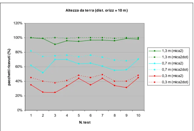
During the experiments we performed to analyze the transmission ranges at various data rates, we observed a dependence of the transmission ranges from the mobile devices’ height from the ground. Specifically, in some cases we observed that devices were not able to communicate when located on the stools, they started to exchange packets by lifting them up. In this section we present the results obtained by a careful investigation of this phenomenon. Specifically we studied the dependency of packet loss from the devices’ height from the ground.
As it clearly appears in Figure 4.3-14 the ground height may have a big impact on the quality of communications between the mobile devices.
R1 R Fr esnel Zone Ground Plane D Figure 4.3-13
Specifically the channel power loss depends on the contact between the Fresnel zone and the ground. The Fresnel zone for a radio beam is an elliptical area located between the sender and the receiver. Objects in the Fresnel zone cause diffraction and hence reduce the signal energy. Figure 4.3-13 shows the Fresnel zone for a sender-receiver couple at a distance D. In the figure, R1 denotes the height of the first Fresnel Zone. R1 is highly dependent on the stations distance. These theoretical considerations are aligned with our experimental results.
Figure 4.3-14 shows that Fresnel effect is more sensible for mica2 sensors than mica2dot motes and that packet loss increases when height decreases.
See appendix 7.6 for details.
4.4. Power
consumption
The battery supplies power to the complete sensor node and hence plays a vital role in determining sensor node lifetime. Batteries are complex devices whose operation depends on many factors including battery dimensions, type of electrode material used, and diffusion rate of the active materials in the electrolyte. In addition there can be several nonidealities that can creep in during battery operation which adversely
Altezza da terra (dist. orizz = 10 m )
0% 20% 40% 60% 80% 100% 120% 1 2 3 4 5 6 7 8 9 10 N. test p acc h e tt i r ice vu ti ( % ) 1,3 m (mica2) 1,3 m (mica2dot) 0,7 m (mica2) 0,7 m (mica2dot) 0,3 m (mica2) 0,3 m (mica2dot) Figure 4.3-14
The most important factor that affects battery lifetime is the discharge rate or the amount of current drawn from the battery. Every battery has a rated current capacity specified by the manufacturer. Drawing higher current than the rated value leads to a significant reduction in battery life. If the high discharge rate is maintained for a long time, the electrodes run out of active materials, resulting in battery death even though active ingredients are still present in the electrolyte.
The effect of high discharge rates can be mitigated to a certain extent through battery relaxation. If the discharge current from the battery is cut off or reduced the diffusion and transport rate of active materials catches up with the depletion caused by the discharge. This phenomenon is called relaxation effect and enables the battery to recover a portion of its lost capacity.
There are two common battery technologies that are applicable for wireless sensor networks: Alkaline and Lithium.
Alkaline Battery for mica2 is rated at 1.5 V, but during operation it ranges from 1.65 to 0.8 V as shown in Figure 4.4-1 and is rated at 2850 mAh. While providing a cheap, high capacity, energy source, the major drawbacks of alkaline batteries are the wide voltage range that must be tolerated and their large physical size. Additionally, lifetimes beyond 5 years cannot be achieved because of battery self-discharge. The shelf-life of an alkaline battery is approximately 5 years.
Lithium batteries provide an incredibly compact power source. The smallest versions are just a few millimeters across. Additionally, they provide a constant voltage supply that decays little as the battery is drained (Figure 4.4-1). Devices that operate off of lithium batteries do not have to be as tolerant to voltage changes as devices that operate off of alkaline batteries. Additionally, unlike alkaline batteries, lithium batteries are able to operate at temperatures down to -40 C. The most common lithium battery is the CR2032 (used for mica2dot motes) ; it is rated at 3V, 255 mAh and sells for just 16 cents.
Theoretically a 1000 mAh battery can suffer a consumption of 10 mA for 100 hours; however in the real usage this consideration is false. Due to the chemical composition of the battery voltage current levels can vary depending on the way energy is extracted from battery.
Furthermore a battery is considered discharged from manufacturer when voltage gets down to 0.8 V (cut-off voltage) even if the circuit that battery stokes may require a minimal voltage greater than 0.8 V.
A very important parameter to be considered in the choice of battery type is that mica2 and mica2dot processor (ATMega128) must be stoked with at least 2.8 V. This forces a limitation in the usage of alkaline batteries that provide a wide voltage range
In details batteries used for the following tests are:
- Panasonic Alkaline AM-3PI ( 1.5V ) ; rated capacity : 2870 mAh (for mica 2) - Panasonic Lithium Coin CR2354 ( 3V ) ; rated capacity : 560 mAh (for mica2dot) - Energizer Lithium AA 2 Pack ( 1.5 V ) ; rated capacity : 2900 mAh (for mica2)
Figure 4.4-1
Due to the wide voltage range of alkaline batteries and the limitation of the ATMega processor described below a first test is a typical battery discharge test.
A mica2 mote in which an application that through an internal counter sends 51-byte pck/sec , is linked to a voltmeter to measure voltage . Furthermore a receiver, placed
quite near (10 m from the sender) , blinks a led if the packet has received ; this simple mechanism allow to know visually when communication stops.
Battery Discharge 0 0,5 1 1,5 2 2,5 3 3,5 0 50 100 150 200 250 time ( hours ) v o lt ag e ( V )
discharge CPU threshold working threshold
Figure 4.4-2
As Figure 4.4-2 shows even if CPU threshold is 2.7 V with a consequent lifetime of 40 hours until 2.3 V motes communicate properly. The conclusion is that the real lifetime is about 150 hours.
Measuring average leaked current for this application we obtain a value of 15 mA , so:
lifetime = rated capacity / load current = = 2870 mAh / 15 mA = 191 h
Between theoretical lifetime and measured lifetime there is a 0.784x factor ; so a good value for effective capacity could be 2250 mAh ( rather than 2870 mAh ). This approximation is very precautionary seeing that real motes application have an average leaked current of about 0.1 mA.
We are going to analyze average leakage current of motes subsystems in different operating conditions.
The reference circuit for measurement is shown in Figure 4.4-3
Figure 4.4-3
Current is measured with an amperometer in series with power supply ( that has an internal impedence) and the mote.
In a first group of tests we analyze different power consumption in different radio operating modalities (transmitting, receiving, idle). It is also considered the special power down mode (referred to the processor state).
Results (Figure 4.4-4) show that:
- mica2 need more energy than mica2 in all working modalities;
- transmit is more expensive than receive ( 18mA VS 16mA in mica2 and 14mA VS 12mA in mica2dot );
- computation ( processor only ) costs 8 mA;
Power Consumption 12 14 11 13 8 0,01 16 18 15 15 8 0,01 0 2 4 6 8 10 12 14 16 18 20 Rec eption Tran smi ssion Idle ( ra dio rx m od. ) Idle (rad io tx mod ) Idle (rad io of f ) Idle (po wer do wn) modality le ake d cu rr en t (m A) mica2dot mica2 Figure 4.4-4
Result in Figure 4.4-4 are the summary of some tests reported explicitly in appendix 7.8.
Both mica2 and mica2dot motes have subsystems as described in 3.1.
In succeeding tests we are interested in power consumption of LED and datalogger component.
Datalogger component that is flash memory on chip can be used as a permanent memory as program memory or temporary data storage. However due to the fact that is persistent no energy is required to maintain data but there are long times and big power consumption for writing and reading (see Figure 4.4-5).
Static RAM on motes could be used for similar purpose but it requires energy to maintain data and it’s a volatile memory even if we have a small access time.
Subsistems leaked current 9,5 15 24 0 5 10 15 20 25 30
CPU+Led CPU+log write CPU+log read active subsistem cu rr ent ( m A ) Figure 4.4-5
As it was said in chapter 3 mica2 and mica2dot support a sensor board where a certain number of sensor can be placed. We are going to measure average leaked current with different sensors ( Figure 4.4-6 )
Power Consumption : sensors
10 9 12 10 0 2 4 6 8 10 12 14
CPU+Sounder CPU+accelerometee CPU+magnetometer CPU+photo subsistem and sensor
cu rr ent ( m A )
Finally we have tested power consumption in a real sensor application.
Mica2 mote samples light through photo sensor every second and transmits an 8-byte packet via radio with the value sampled. When radio is not used radio is put off and processor enters in power down mode.
Test is done in default condition so with 0 dB/mW power out and in an indoor environment.
If we graph current trend we obtain Figure 4.4-7 .
A real application 0 5 10 15 20 25 0 1 2 3 4 5 6 time (s) c u rre n t (m A) Figure 4.4-7
It is quite clear that when sampling leaked current is 20mA while in transmitting mode is 18 mA.
When mote is in power down mode current decades to 10 uA.
If we consider one period average current leaked is 0.19 mA; thus causes a power leaked of 0.57 mW (that is 0.19mA * 3 V). Using typical lifetime found in initial power consumption test we have the following lifetimes:
Lifetime ( alkanine battery ) = 11800 h = 1 year and 3 months
Lifetime ( lithium battery ) = 15263 h = 1 year and 7 months
4.5. Throughput
In this section we will show that only a fraction of the 19.2 Kbps nominal bandwidth can be used for data transmission. To this end we need to carefully analyze the overheads associated with the transmission of each packet (see Figure 4.5-1).
From the figure we can note that a certain number of send application calls go into a queue. With a FIFO politic packets are passed to MAC layer and the to the physical one. Each layer produce an acknowledgment to the upper level until send is considered done when application receives the ack.
Figure 4.5-1
Specifically each maximum 36 bytes generated by a legacy TinyOS application is encapsulated by the MAC-layer that adds a 18-bytes preamble and 2-bytes synchronization information for transmission over the wireless medium. We could differentiate two kind of throughput depending on which part of the packet we consider useful (see Figure 4.5-2):
- throughput : if we consider the whole 56-bytes as useful;
Figure 4.5-2
If we consider packets of maximum data size whereas effective data radio rate is 19.2 kbps packet time is 23.3 ms (that is 43 packets / s) :
packet time = 56 byte / 19.2 kbps = 23.33 ms
With this observation we can simply compute theoretical throughput :
Throughput = 19.2 kbps (obvious !) Net Throughput = 12.4 kbps
Tests with 2 stations at 10m distance show that measured throughputs are very near to theoretical ones (Figure 4.5-3).
It is very important to note that in these experiments MAC delay is fixed to 0 so we haven’t any delay due to MAC overhead.
Throughput 19,2E+3 19,1E+3 12,4E+3 12,3E+3 000,0E+0 5,0E+3 10,0E+3 15,0E+3 20,0E+3 25,0E+3 kbp s theoretic throughput avg. measured throughput theoretic net throughput avg. measured net throughput
Figure 4.5-3
Now we consider the MAC delay due to random initial backoff ( see 3.2.8 ) . In a theoretic point of view we can differentiate:
- Theoretic minimum net throughput: it’s computed considering the initial backoff time fixed to the maximum value (68.3 ms) . We obtain a value of 3.2 kbps. - Theoretic maximum net throughput : it’s computed considering the initial backoff
time fixed to the minimum value (15 ms). We obtain a value of 7.6 kbps.
- Theoretic average net throughput : it’s computed considering the average backoff time ( (68.3+15.2) / 2 = 41.75). We obtain a value of 4.5 kbps.
Theoretic minimum net throughput = 3.2 kbps Theoretic maximum net throughput = 7.6 kbps Theoretic average net throughput = 4.5 kbps
The average measured throughput is very near to the theoretic one (Figure 4.5-4) Throughput 7,6E+3 4,5E+3 3,2E+3 4,6E+3 000,0E+0 1,0E+3 2,0E+3 3,0E+3 4,0E+3 5,0E+3 6,0E+3 7,0E+3 8,0E+3 k bps
theoretic max net t. theoretic average net t. theoretic min net t. average measured net t.
4.6. Software
overhead and time analysis
In this section we would like to measure through experiments the overhead introduced by TinyOS stack protocols and evaluate times during a transmission. Fist we must consider that when a motes (A) transmits a packet to another mote (B) there are several times to count (Figure 4.6-1) :
- t stack down : it’s the time to cross TinyOS stack protocol from up to down. - t FIFO queue : it’s the time that a packet spends in the FIFO queue. It’s 0 if queue
is empty.
- t MAC delay : it’s the time introduced by MAC layer. It could be set to 0 or it’s controlled by MAC layer (so it can be initial backoff time or congestion backoff time).
- t packet time : it’s the time needful for packet transmission. It is related to radio effective data speed. We can assume it to 23.3 ms for a maximum length packet. - t propagation delay : it’s the time of signal propagation in the air
Figure 4.6-1
A first set of experiments show that propagation delay is negligible respect other times.
In fact propagation delay is defined as distance divided speed of light in the air:
propagation delay = D / v
where :
D = distance between motes
v = speed of light in the air = 298000 km/s
From Table 4.6-1 we can see that propagation delay has a magnitude order of 10^-8 , 10^-9 while other times are 10^-3 ; so it can be omitted.
D(m) Tpd(s)
10 3,36E-08 50 1,68E-07 100 3,36E-07
Table 4.6-1
In all following tests it’s important to notice that all time are application to application related; this is due to the fact that we operate at application level thought TinyOS programs.
Now we consider one station; the mote is programmed with a TinyOS application that starts a timer and transmits a 36-byte packet through a Send() call ; the mote stops the timer when application receives SendDone() signal ( Figure 4.6-2 ).
Figure 4.6-2
Results show that averaged time measured is 26.15 ms. So we can conclude that software overhead is about 2.85ms since packet time is 23.3 ms. In fact until motes haven’t send the last bit it doesn’t send the acknowledgment to application level ( sendDone() ).
It’s important that MAC delay is fixed to 0 so we haven’t the aleatory of MAC layer.
If we have a 2 station configuration we can estimate the application to application RTT (round trip time) (refer to
Figure 4.6-3)
Figure 4.6-3
In this case A starts a timer and transmits a 36-byte packet to B that resends it to A. When A receives the packet stops the timer and compute the RTT time.
The result RTT is of 52.4 ms so this time software delay is about 5.8 ms.
This fact can be explained if we think that there are four crossings of protocol’s stack: - A crosses stack from up to down to send the packet;
- B crosses stack from down to up to receive the packet; - B crosses stack from up to down to resend the packet;
- A crosses stack from down to up to receive the packet sent by B;
Finally consider a 4-station configuration in which stations forward the packet.
A starts a timer when transmits a packet to B. When A receives back the packet it stops the timer and computes the RTT time (Figure 4.6-4)
Measured RTT is 156.95 ms so software delay is about 17.15 ms; this is due to many crossings of protocol’s stack.