S TEERABLE C ONCENTRIC R ING A RRAYS 1 C ONSTRAINED P ARETO O PTIMIZATION OF W IDE B AND AND

1 C

P

O

W

B

S

C

R

A

A multi-objective evolutionary algorithm that explicitly introduces the management of a single or multiple constraints on the solutions of an electromagnetic problem is presented in his chapter. The proposed strategy is based upon a modified genetic algorithm which evaluates the strength of a solution by considering both the match to the desired performance (objectives) as well as the satisfaction of specific requirements imposed to the design (constraints). The key issue is represented by the adaptive constraints management and its influence on the selective pressure of the genetic algorithm. The procedure is applied to the optimization of concentric ring arrays. Several design examples of steerable and wideband arrays are provided to prove the flexibility and reliability of the approach. A particular emphasis is given to the changes in array performance when the same objectives are requested but different kinds of constraints are forced.

Multi-objective evolutionary algorithms (MOEAs) are efficient for simultaneous optimization of conflicting design objectives. A multi-objective design differs from a single-objective problem where a global minimum or maximum represents the best solution. In fact, in the case of multiple cost functions a solution that fully satisfies all the requirements may not exist. Moreover, a change in the design parameters representing an improvement for one objective can cause, at the same time, a deterioration to another one. For this class of problems, there exists an ideal set of solutions, named the Pareto Front (PF), over which no other solution of the population dominates [1]. MOEAs have been recently adopted in the electromagnetic community to design linear arrays with low sidelobe level and narrow half-power beamwidth [2][3], antennas with high gain or small size [4][5], microwave absorbers with a high level of attenuation and a small thickness [6]-[8]. The opposing but desired objectives have to be pursued by choosing the value of the physical parameters in the limited range of allowed values. Within this framework, a further level of challenge can be represented by a multi-objective optimization where some additional constraints have been explicitly imposed to the decision variables, thus reducing the extent of the total search space [8][9]. This can be the case of planar array designs where it is not only necessary to obtain low Peak Sidelobe Levels (PSLLs) and predefined Half-Power Beamwidths (HPBWs) at a fixed

frequency band, but also to take into account other constraints such as the efficiency or, for instance, a maximum number of the radiating elements.

In this work we are interested in designing Concentric Ring Arrays (CRAs) by introducing a flexible and general management of constraints in a multi-objective electromagnetic problem. We focus our attention on arrays able to fulfil requirements such as a low PSLL or a large Fractional Bandwidth (FBW). At the same time we restrict our search for optimized antenna arrays that comply additional criteria for their practical realization such as a minimum inter-element spacing and a constrained limited number of radiating elements. This chapter is organized as follows. Section 1.1 illustrates the implemented multi-objective genetic algorithm which is capable of explicitly managing constraints imposed by the designer, both of equality and inequality. Then, Section 1.2 describes the properties of CRAs and the geometrical parameters which define the radiating structure. The following Section 1.3 assesses the proposed algorithm performance using a CRA design as a test case. Section 1.4 provides some design examples of planar arrays which allow highlighting the reliability of the optimization procedure as well as the effectiveness of the constraint enforcement. Finally, some concluding remarks are given.

1.1 Constrained Pareto Optimization

As all evolutionary algorithms, the MOEAs are useful when the design requires managing a large number of parameters and the presence of multiple and divergent objectives. Let us suppose there are K objective functions fi (x), which require to be simultaneously

optimized (i.e. minimized or maximized), where the variables xn can assume values in a

N-dimensional search space defined by boundaries:

 





By recurring to the Pareto dominance concept, it is possible to determine a set of optimal solutions known as the Pareto Front. More in detail, in the case of a minimization of the objectives, a solution x1 is defined to dominate another solution x2 if and only if the objective function values for x1 are less than or equal to those of x2, and at least one is strictly

less than that of x2. This set provides a range of solutions representing a trade-off of the desired design objectives but none of these solutions can be considered the best of all, thus the designer has to find as many Pareto-optimal solutions as possible to determine the front [1]. The Paretofront search could be accomplished by recurring to a single-objective algorithm where each one of the many objectives is emphasized at time. However, this requires many singleobjective simulation runs and does not guarantee an efficient scouting of the Pareto front [10],[12]. On the contrary, a MOEA is able to find multiple Pareto-optimal solutions in a single run. In the last years, several optimizers based both on Genetic Algorithm (GA) [13][14] and Particle Swarm Optimization (PSO) [15][16] have been employed to handle multi-objective problems.

Within this framework, the problem of constraints handling has received more and more attention in the optimization literature and a large number of solutions have been proposed [17]-[19] to take into account the imposed constraints throughout the optimization process. Constraints may involve physical limitations imposed to certain parameters and determine a reduction of the allowed search space. They can be generally divided into two classes, namely inequality vj(x) and equality uj(x) constraints:

 





 





where s is the number of inequality constraints and (t-s) that of equality ones. As a result, we can have a feasible solution and an infeasible one whether all the constraint goals are accomplished or not. More in detail, a feasible solution must satisfy (1.2), regardless of the values assumed by its objectives, whereas an infeasible one may have a better performance but does not fulfil (1.2). It is worthwhile to underline that an infeasible solution is a solution that does not adhere to our constraints but nevertheless has a physical meaning.

In this work, we adopt a modified implementation of the Non-dominated Sorting Genetic Algorithm II (NSGA-II) [17] with the constraint management approach proposed in [20]. The flow chart of the algorithm is shown in Figure 1.1 and it will be hereafter illustrated. An initial population of M chromosomes is randomly generated at the beginning of the evolutionary process. Next, the value of each one of the K objective functions is evaluated for

each solution codified in the genetic pool. In the absence of any constraints only this contribute provides the dominance criterion necessary to pursue the Pareto front however, if some constraints are enforced, the algorithm has to be modified to pursue solutions satisfying the imposed limitations. The key point of our modified algorithm is to not discard a priori all the infeasible solutions because some of them may possess some useful information. In fact, the modified calculation of the objective values is based on the relation between a careful estimate of the degree of violation of the imposed constraints and the level of performance expressed by the objectives value. These tasks are accomplished by the use of a suitably defined distance and an adaptive penalty. For this purpose a normalized objective function needs to be defined, where the operators min

 

x and Maxx  apply on the current population:

 

 



 



 







 



The constraint violation w(x) of a solution coded in a chromosome is defined as well on the current population as the normalized summation over all the constraint violations

 

 

 

 



 



 



 





being  the tolerance value accepted for the equality constraints. It is apparent from (1.5) that

cj(x) is greater than zero only when the individual violates the jth-constraint. At this point, a

new distance can be introduced in each one of the N dimensions as

 

 

 

 

where F is the ratio between the number of feasible solutions in the current population and the population size M. The adaptive penalty further modifies the objectives evaluation of infeasible solutions. The aim of this term is to properly consider the infeasible solutions without discarding or equally penalizing all of them a priori. The correction term for the

ithobjective function dimension is expressed by

 





 

 

 

_{ }

 

_{ }

The adaptive nature of (1.7) is apparent from (1.8) and (1.9). In fact, when there is a small number of feasible solutions, chromosomes with higher constraint violations are more penalized than those with lower ones. Similarly, when F is large, infeasible solutions will be penalized on the basis of a high objective function value. Therefore, this adaptive penalty term initially stimulates the search of feasible solutions and then improves them. It is worthwhile to notice that the switch between these two goals can happen anytime during the evolutionary process thus avoiding to manually tune parameters for this task. The final modified objective function in the ith-objective function dimension is expressed by

 

 

 

i i i

MF x dist x p x (1.10)

and it allows an efficient employment of the unfeasible solutions to improve the search. More in detail, the adaptive nature of (1.10) does not always prefer chromosomes with small constraints violation only or with low objectives value only. If the pool contains only infeasible solutions, the modified objective function in (1.10) pushes the evolutionary process toward the search of feasible individuals before searching for the individuation of configurations that improve the objectives. It promotes individuals with both low objective function values and low constraint violations with respect to those with higher values of objectives and/or violations. When two chromosomes have close distance values disti(x), the

dominance is mainly influenced by the penalty term pi(x). In fact, if F is small the solution

closer to the feasible space will be the dominant one; on the contrary, if F is large, the solution with the smaller objective function value will prevail.

Once the modified function values have been calculated for all the M chromosomes in the pool, the standard NSGA-II is employed. The nondominated sorting is then applied to the population and it determines the actual Pareto front and the other ranked partitions. Following the described steps the initial parental generation with M chromosomes, Parent(M,0), is generated. Next, at each iteration k an offspring, Offspring(M,k), is generated by using the well-known tournament selection, crossover and mutation operators [21], while Parent (M,k) is temporary stored. The modified objective functions of Offspring(M,k) are then evaluated and both the parental and the offspring pools are merged into Union (2M,k) and sorted. In order to reduce the population to M members, it is necessary to apply the

crowdedcomparison operator which measures the uniformly spread-out of the solutions on the Pareto front [17]. Until the maximum number of generations is reached the set of chromosomes represented by Union (M,k) is considered as the input Parent (M,k+1) and further optimized.

1.2 Concentric Ring Arrays Optimization

Unlike linear arrays that can only scan the main beam in one polar plane, planar arrays offer the advantage of a 3D scanning of the main beam and this feature is required in a large variety of applications such as wireless communications, air navigation, radar and radio astronomy. A low peak sidelobe level and a narrow half-power beamwidth are often included in the requirements and many options are available to the designer to accomplish them. Periodic planar arrays can be tailored to possess a low PSLL even if at the cost of a narrow bandwidth, while completely random arrays may offer a wider range of frequencies but they suffer from a limited ability to predictably control the worst case of PSLL. Moreover, a totally random array increases the complexity of the feeding network. In order to allay these drawbacks, it is possible to recur to an amplitude tapering [22]-[24] or a phase tapering [25] [26], for those cases where the element lattice is fixed and elements are equally spaced. Other techniques exploit unequally spaced array [24]-[27] or the perturbation of a particular geometry [28] since irregular arrays provide a way to address grating lobe problems by eliminating the periodicities in the element locations. All the aforementioned techniques may be also jointly employed [29][30] in order to get additional degrees of freedom in the design.

Among the possible planar array configurations, the Concentric Ring Array (CRA) exhibits the interesting properties of a nearly invariant pattern for a full azimuthal coverage and main beam symmetry. An example of a generic CRA is given in Figure 1.2, where P is the total number of rings, rp is the radius of ring p and dp is the constant distance between the

elements in the ring p. The use of CRA providing main lobe scanning has been addressed by using current amplitude tapering [31] and space-tapering [32][33], by optimizing both current amplitudes and ring spacing [34] or rings spacing and number of elements in each ring [35]. Within this framework, our aim is to employ our MOEA to design CRAs with requirements imposed on the PSLL and HPBW under the presence of explicit inequality or equality

constraints. In the next section the flexibility and reliability of the proposed optimization method will be illustrated by examples with a constraint on the number of elements in the array and on the beamwidth when steering in the desired direction.

Figure 1.2 - Geometry of a concentric ring array.

In particular, we focus most of our attention on antenna arrays with a controlled or maximum number of elements. We do not employ any amplitude tapering and we just control the phase to point the main beam in the desired direction since this solution guarantees a simple feeding network and maximizes the total radiated power for a given number of radiating elements. We also require that the proposed solution is physically realizable, thus the minimum distance between elements in the array has to be set consistent with the overall antenna dimension both to satisfy mechanical limits imposed by element size and to mitigate the effect of electromagnetic coupling.

1.3 Concentric Ring Array Design as a Benchmark for Multi-objective

Constrained Optimization

In order to assess the performance of our MOEA the proposed algorithm is tested on an EM design problem. More in detail, we provide a comparison with the Non-dominated Sorting Genetic Algorithm II (NSGA-II) [17] by focusing on the design of a concentric ring array regarding the minimization of the PSLL and the HPBW under the imposed constraint of

N =50. The NSGA-II algorithm has been chosen as a benchmark since it has proven to

outperform two other recent MOEAs such as the Pareto-Archived Evolution Strategy (PAES) [36] and the Strength-Pareto Evolutionary Algorithm (SPEA) [37]. In the case of the

aforementioned NSGA-II, the constraints are directly involved in the Pareto dominance definition. In particular, the result of the comparison between two solutions x1 and x2 (in the case of a minimization of the objectives) is determined by the following rules:

 if one solution is feasible (x1) and the other (x2) is infeasible, then x1 dominates x2, regardless of their objective function values;

 if they are both feasible solutions the standard Pareto dominance is applied which means that a solution x1 is said to dominate another solution x2 if and only if the objective function values for x1 are less than or equal to those of x2, and at least one is strictly less than that of x2;

 if they are both infeasible solutions but one solution (x1) has less constraint violation than the other solution (x2) then x1 dominates x2.

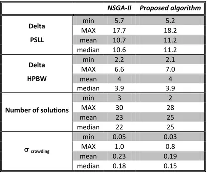
Therefore in NSGA-II case, the level of constraint violation is used to compare two infeasible individuals and thus the non-dominance ranking ignores the values assumed by those individuals in the objectives space and this may cause in a possible loss of some important evolutionary material. We have performed 100 multi-objective genetic algorithm optimizations with both the NSGA-II and the proposed algorithm. Each one of the 100 runs comprises 1000 generations. With a population size of 100 chromosomes, the total number of unique fitness evaluation is 1x107, which is sufficient to justify its effectiveness from a statistical perspective. More in detail, for each solution on the final PF produced by the 100 runs we have evaluated:

 maximum and minimum difference between the peak sidelobe level (PSLL) values of the two extreme points of the PF (referred as Delta PSLL) as well as arithmetic mean and median of the PSLL;

 maximum and minimum difference between the half power beam width values of the two extreme points of the PF (referred as Delta HPBW) as well as arithmetic mean and median of the HPBW;

 maximum, minimum, mean and median of the number of the solutions in the final PF;

 maximum, minimum, mean and median of the standard deviation of the crowding distance ( crowding ) of the solutions forming the PF.

These parameters have been chosen since they provide a significant indication of the diversification among the individuated EM designs and the spreading of the solutions along the Pareto front. In fact, the Delta PSLL and the Delta HPBW quantitatively describe the extension of the Pareto front and the excursion of the objectives along each search direction. A greater excursion means the designer has more freedom of choice in terms of solutions with different performance, whereas it is obvious that a higher number of solutions is preferable. Finally, since the crowding distance [17] provides the density estimation of solutions surrounding a particular solution in the population, the smaller the value of its standard deviation the more homogeneous is the distribution of the solutions along the Pareto front. The final results are reported in Table I.

Table I - Comparison between NSGA-II and the proposed algorithm

NSGA-II Proposed algorithm

Delta PSLL min 5.7 5.2 MAX 17.7 18.2 mean 10.7 11.2 median 10.6 11.2 Delta HPBW min 2.2 2.1 MAX 6.6 7.0 mean 4 4 median 3.9 3.9 Number of solutions min 3 2 MAX 30 28 mean 23 25 median 22 25 crowding min 0.05 0.03 MAX 1.0 0.8 mean 0.23 0.19 median 0.18 0.15

As observed from Table I, the proposed algorithm exhibits some advantages with respect to the NSGA-II for the addressed problem of concentric ring array design. First of all, the mean and median Delta PSLL is better whereas the Delta HPBW is the same for both algorithms. The number of solution is 12% higher in the case of the proposed algorithm and

the  crowding is 17% less than that of the NSGA-II which means that the solutions have a more homogeneous spread along the PF. The percentage values are calculated with respect to the median values since this parameter is less influenced by extreme values that may be present in the distribution.

1.4 Optimization Results: Concentric Ring Array synthesis

This section addresses the application of the proposed MOEA to different concentric ring array designs. The number P of rings, their radius rp and the number of elements in each

ring are some of parameters under designer's control that need to be optimized. The radius of each ring has to be independently selected as well in order to enhance the array performance. The elements in each circle are uniformly spaced in angle therefore another choice regards the ring angular offset which breaks the alignment of radiating elements in each radial direction thus improving the robustness of the solution with respect to the PSLL. All the antenna arrays considered here are assumed to be composed of uniformly excited isotropic elements with inter-element spacing in [0.5,  A population of 100 chromosomes is chosen to approximate the PF to provide a large number of trade-off configurations to the designer. The described synergic use of infeasible and feasible solutions in the genetic pool guarantees a good rate of convergence: a number of 1000 iterations has been found suitable for the evolutionary process. More in details, we focus our attention on three optimization examples which are carefully investigated to prove the usefulness of the proposed MOEA to the EM design of CRAs. In the first example, the relation between the peak SLL and array beamwidth is addressed for a CRA with maximum radius 4 by varying the radius of each ring and both

the total number of rings and elements in each ring. As an example of handling constraints in the evolutionary process, we set the total number of array elements by using an equality constraint as well as an inequality constraint. As a second test, we perform the optimization of a CRA with a given minimum beamwidth for broadside radiation and we aim to minimize, at the same time, its peak SLL both at broadside and at 60° steering. Finally, in the third example, two optimizations of a CRA are performed to achieve a wideband array with a fractional bandwidth greater than 0.5. In the former we apply an equality constraint on the

beamwidth in broadside direction, while in the latter we additionally introduce a limitation on the number of radiating elements.

1.4.1 Constrained optimization of PSLL and HPBW

Let us consider a CRA with maximum radius 4 and a given number N of sources. The objectives are the minimization of the peak SLL and a HPBW as narrow as possible while an equality constraint of N = 80 is applied. Generally, the problem without imposing any constraints on the element number does not require a multi-objective optimization tool since given an aperture, increasing the number of radiating sources usually leads to a decrease of both the SLL and the HPBW. On the contrary, setting a constraint on the number of elements changes the problem from single-objective into multi-objective.

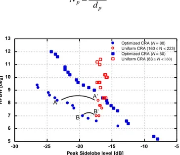
The final Pareto front associated with this optimization process is reported in Figure 1.3. In order to have a comparison, each optimized array that belongs to the Pareto front is mapped into a uniform CRA covering the same area. More in detail, for a uniform concentric ring array the spacing dp between elements in a ring, is approximately constant for all rings and the

ring spacing rp is proportional to dp. By setting dp equal to 0.5the number of elements in

each ring of the uniform ring array is equal to

2 _p p p r N d   (1.11). 5 6 7 8 9 10 11 12 13 -30 -25 -20 -15 -10 -5 Optimized CRA (N = 80) Uniform CRA (160  N < 223) Optimized CRA (N = 50) Uniform CRA (83 N <  H P B W [d e g]

Peak Sidelobe level [dB]

A

A' B

B'

Figure 1.3 - Comparison in terms of performances between the optimized Pareto and almost uniformlyspaced solutions.

It is obvious that the number of elements in the uniform CRA is greater than the one of the optimized CRA. Thus the uniform CRAs consist of a number of elements ranging between 83 and 223. The performance of these uniform CRAs have been mapped in Figure 1.3 and it is apparent that the curve for the uniform arrays is completely dominated by the Pareto front relative to N = 80, which indicates that the optimized CRA has a lower SLL than a uniformly spaced periodic array with the same beamwidth. If we apply an equality constraint of N = 50, the new PF is dominated by the PF found for the solution related to N = 80 (Figure 1.3) but always outperforms the uniform counterparts comprising less than 160 elements, for a corresponding reduction of the radiating sources from 40% to 68%. Moreover, a uniform array with more than 160 elements cannot guarantee a peak SLL lower than 17.6 dB. The spread of the solutions along the PF guarantees in both cases (N = 80 and N = 50) a wide set of choices to the designer. It is also important to underline that the optimized array not only results into a more cost-saving design but it may ensure a comparable directivity even if it possesses fewer elements than the corresponding uniform array. As an example, designs A and

B are two non-dominated designs comprising 80 elements and arbitrarily selected from the

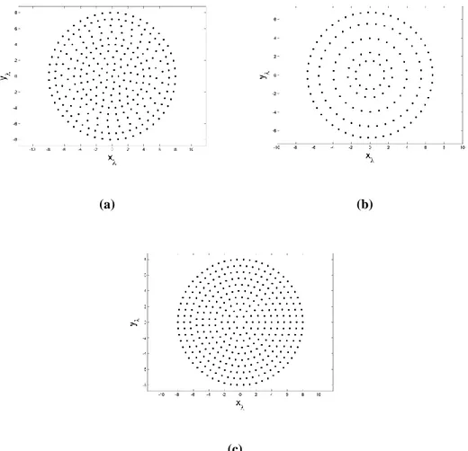
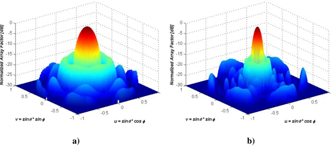
Pareto front, with maximum radius of 3.4 and 3.8, respectively. Compared to uniform arrays with the same aperture sizes, A’ and B’, the optimized arrays have similar beamwidths but significantly reduced peak SLLs. Their geometrical structures as well their correspondent Array Factors (AFs) are plotted in Figure 1.4 and Figure 1.5 where the coordinates (X, Y) are expressed in the term of free space wavelength 

-40 -35 -30 -25 -20 -15 -10 -5 0 -1 -0.5 0 0.5 1 A F [dB] Sin(Theta) (c)

Figure 1.4 - Comparison between antenna layout and array factor of two designs: a) the optimized 80element CRA A, b) its corresponding uniform 160element CRA A’, c) array factors ( = 0 deg.) for optimized array (continuous line) and for uniform CRA (dashed line).

-40 -35 -30 -25 -20 -15 -10 -5 0 -1 -0.5 0 0.5 1 A F [dB] Sin(Theta) (c)

Figure 1.5 - Comparison between antenna layout and array factor of two designs: a) the optimized 80element CRA B and b) its corresponding uniform 223element CRA B’, c) array factors ( = 0 deg.) for optimized array (continuous line) and for uniform CRA (dashed line).

The peak SLL improves from 17.1 dB (uniform case A’) to 23.4 dB (optimized case A) while the directivity is almost the same (26.49 dB for A and 26.6 dB for A’). However solution A’ has 160 elements, twice the number of elements in design A. The uniform array B’ is composed of 223 elements and it exhibits a peak SLL of 17.4 dB, whereas design B possesses almost one third of all the elements with a much lower SLL equal to 19.6 dB. In this case, the directivity decreases from 28.3 dB to 25.6 dB which is clearly due to the high reduction (77%) of the number of radiating sources.

4 6 8 10 12 14 16 18 -25 -20 -15 -10 -5 N=30 20N 29 H PB W [ d eg]

Peak Sidelobe Level [dB]

Finally, a further study of the PF in the case of arrays with N = 30 or less has been performed for the same maximum radius of 4and the results shown in Figure 1.6 prove the reliability of the optimization process to find also in this case configurations with low peak SLL.

1.4.2 Constrained optimization of SLL for broadside and steered direction

It is well known that for a planar antenna array optimized to point at a given direction, the beamwidth changes according to the orthogonal projection of the aperture size while the peak SLL cannot be analytically predicted as well. A multi-objective optimization can be therefore employed to search planar array with trade-off performances for a set of different pointing directions. As an example, at a given frequency f0, a two-objective NSGA-II is

applied to simultaneously minimize antenna array peak SLL at two different main beam steering directions, while imposing a constraint of equality of a HPBW of 15 degrees at broadside operation (with a tolerance value  of 0.4°). The considered directions of the main beam are broadside and 60 degrees from broadside.

The final Pareto front is illustrated in Figure 1.7. This front consists of CRAs fulfilling the equality constraint imposed over the HPBW but with a different number of elements since no constraint was applied on it. The performance in terms of peak SLL of these solutions ranges between 24.8 dB and 17.6 dB for broadside scanning and 9.5 dB and 13.7 dB for 60° off broadside scanning. As a comparison, a singleobjective GA has performed two distinct optimizations of a CRA, one for broadside and another one for a steering of 60° from broadside, with the same HPBW requirement. In order to make a fair comparison, the number of fitness evaluations has been set equal to that of the multiobjective case. As expected, the best GA solutions are placed very close to points of the PF (Figure 1.7) but GA provides only one configuration at time while MOEA finds several ones in only one run while maintaining good diversity and spread of solutions.

-14 -13 -12 -11 -10 -9 -25 -24 -23 -22 -21 -20 -19 -18 -17 NSGA-II approach GA approach P e a k S L L (  m ax = 6 0 °) [ d B ] Peak SLL (max= 0°) [dB] Best trade-off solution

Best steered solution Best solution at broadside

Figure 1.7 - Final Pareto front of peak SLL optimization for broadside and steered direction.

Three multi-objective solutions were chosen for further considerations: the first one with considerable SLL suppression at broadside, the second one with a satisfactory SLL trade-off at both the scanning directions and the last one with a good SLL suppression when scanned to 60° off broadside. -2 -1.5 -1 -0.5 0 0.5 1 1.5 2 -2 -1.5 -1 -0.5 0 0.5 1 1.5 2 X  Y  -2 -1.5 -1 -0.5 0 0.5 1 1.5 2 -2 -1.5 -1 -0.5 0 0.5 1 1.5 2 X  Y  (a) (b)

-2 -1.5 -1 -0.5 0 0.5 1 1.5 2 -2 -1.5 -1 -0.5 0 0.5 1 1.5 2 Y  X  (c)

Figure 1.8 - Antenna layouts for three optimized CRAs: a) the best trade-off solution, b) the best broadside configuration and c) the best one when steered to 60 degrees.

The first one is an optimized CRA with 35 elements and a SLL of 24.8 dB at broadside and a 9.5 dB SLL at the scanned direction. The second array comprises 39 elements and exhibits a peak SLL of 22.08 dB at broadside and of 11.6 dB at 60 degree off broadside. The last example is a 40element CRA providing a SLL of 17.6 dB at broadside and

13.7 dB when steered. Layout of these three array designs are shown in Figure 1.8 while their main radiation performance are summarized in Table II.

Table II - Radiation performance of the three CRAs

max = 0° max = 60°

# elements Peak SLL HPBW Peak SLL HPBW

35 -24.8 dB 15.3° -9.5 dB 41°

39 -22.08 dB 14.6° -11.6 dB 35.4°

1.4.3 Constrained Optimization of wideband CRAs

Generally, as the inter-element spacing increases beyond the limit of a wavelength at the operating frequency, the radiation performance is deteriorated due to the arising of grating lobes. However, when each radiating element is arranged within a concentric circular lattice, the appearance of grating lobes can be mitigated and controlled. By exploiting this intrinsic property of the CRA layout, the optimization process has been further employed to synthesize several planar arrays with controlled peak SLL within a specified angular range over a wide frequency range. The frequency range is specified by using the fractional bandwidth (FBW) defined as ( ) / 2 U L U L M M U L f f f f f FBW f f f f       _ (1.12)

where fM, fU and fL are respectively the center, the upper and the lower frequency. According

to (1.12), arrays are considered wideband when 0.2 < FBW < 0.5 and ultrawideband when FBW > 0.5 [30].

In order to obtain a minimization of the peak SLL over a large bandwidth, the radiating points are allowed to have an inter-element spacing in the range [0.8,1.6while the maximum radius has been increased to 8, where  is the wavelength related to the lowest

considered frequency.

Our constrained optimization is then applied to the design of two ultra-wideband CRAs with the goal to jointly minimize the peak SLL when the main beam is scanned at broadside and 60° off the broadside direction. In addition, the value of the FBW has to be maximized with the constraint of a peak SLL not greater than 10 dB in the considered bandwidth. Moreover, in the former design a single equality constraint has been imposed over the beamwidth in broadside direction (HPBW = 3.7° with a tolerance of 0.4°), while in the latter an inequality constraint on the maximum allowed number of elements (N < 150) has been further requested. In order to provide a quantitative measure of the obtained performance both the CRAs has been compared to a third configuration comprising the uniformly 0.8-spaced counterpart fitting the same aperture.

The element arrangements of the three considered designs are represented in Figure 1.9. The optimized design without the limitations imposed on the number of elements comprises 268 elements, while the one satisfying the inequality constraint has 142 sources, resulting in a thinning of about 22 % and 58 % with respect to uniformly spaced counterpart.

(a) (b)

(c)

Figure 1.9 - Antenna layout for three compared designs: a) Optimized 268-element CRA, b) Optimized 142-element CRA, c) Uniform 340-element CRA (inter-element spacing = 0.8

The radiation performance in terms of directivity and SLL for both the optimized scanning directions is illustrated in Figure 1.10, Figure 1.11, Figure 1.12 and Figure 1.13. With respect to the evaluation of the directivity, it is assumed that each element has zero radiation in the lower half-space z < 0. Since the calculation of the directivity by sampling the array factor may depend on the adopted spatial resolution we have calculated the directivity by employing the closed form described in [38]. As apparent from Fig.10 and Fig.11, both the optimized CRAs exhibit a peak sidelobe level lower than the uniform CRA all over the

analyzed bandwidth. This trend remains stable as the main beam direction is steered off broadside. More in detail, by considering the imposed peak SLL threshold of 10 dB the FBW for the first configuration (268 elements) is equal to 1.8 while the array with the constraint on the number of elements (142 sources) exhibits a FBW of 1.7. The directivity of the optimized layouts is slightly less than that of the uniform one because, especially in the case of the 268-elements design, the average loss in directivity is not greater than 1.0 dB, while the peak SLL is consistently reduced. -18 -16 -14 -12 -10 -8 -6 0 5 10 15 20

Uniform (broadside) - 340 elements

Optimized (broadside) - 268 elements

Optimized (broadside) - 142 elements

P e a k SL L (d B ) f/f o

Figure 1.10 - Peak sidelobe level as a function of frequency for the designs shown in Figure 1.9, when scanning at broadside. -18 -16 -14 -12 -10 -8 -6 0 5 10 15 20

Uniform (steered) - 340 elements

Optmized (steered) - 268 elements

Optimized (steered) - 142 elements

P e a k SL L (d B ) f/f o

Figure 1.11 - Comparison of the peak sidelobe level as a function of frequency for the designs shown in Figure 1.9, when steered to 60° from broadside.

22 23 24 25 26 27 28 29 30 31 32 33 34 0 5 10 15 20

Uniform (broadside) - 340 elements

Optimized (broadside) - 268 elements

Optimized (broadside) - 142 elements

f/f o D ir e c ti v it y (dB )

Figure 1.12 - Comparison of the directivity as a function of frequency for the designs shown in Figure 1.9 at broadside. 22 23 24 25 26 27 28 29 30 31 32 33 34 0 5 10 15 20

Uniform (steered) - 340 elements

Optimized (steered) - 268 elements

Optimized (steered) - 142 elements

f/f o D ir e c ti v it y (dB )

Figure 1.13 - Directivity as a function of frequency for the designs shown in Figure 1.9 - Antenna layout for three compared designs: a) Optimized 268-element CRA, b) Optimized 142-element CRA, c) Uniform 340-element CRA (inter-element spacing = 0.8

when steered to 60° off broadside.

The illustrated examples prove the effectiveness of the algorithm in designing concentric ring arrays with optimized HPBW and peak SLL for different scanning directions and even with ultra wide band behavior. The influence of the imposed constrained on the overall performance of the optimized structures has been carefully addressed and it provides a further meaningful degree of freedom for practical designs.

since no assumptions were made about the number of objectives and constraints that is arbitrary.

1.5 Wideband Spiral Array synthesis

One more attractive strategy to the design of non-uniform arrays is to consider deterministic aperiodic structures generated through some mathematical rule and number theory, that manifest unique element localization and properties. To this class of configurations belong for example, aperiodic planar arrays described by a deterministic law and generated by sampling a self-similar geometry like a spiral [39], whose scalable structure can have intrinsically wideband properties. A major advantage of self-similar spiral arrays compared to completely randomised ones, is the reduced construction costs as a result of the minimisation of conduits, power cables, optic fibres, etc., obtained by following the spiral path. As the spiral array can be interpreted as a particular case of the more general CRA, ee have adopted the multi-objective genetic algorithm to optimize the array factor of a Spiral Array.

The structure to be optimized by using the multi-objective algorithm NSGA-II is a spiral array. Our aim is to minimize the sidelobe level (SLL) within a specified frequency bandwidth and inside the suppression region, while steering main beam at broadside direction. The suppression region is made up of all the (u=sinsin ; v=sincos) values in which the SLL needs to be evaluated and minimized as much as possible with the constraint of a fixed number of generations.

The spiral array can be efficiently described by the number of branches, the number of elements on each branch, the maximum radius and the monotonic function r( which indicates how radius changes while increasing distance from the fixed centre point. Given a fixed number M of branches and a frequency range [fmin, fmax], our goal is to optimize the

geometry and number of elements on each branch of a M-branch spiral array of isotropic sources to achieve minimum SLL.

As an example we consider the suppression region described by > 13 degrees. In this case, the imposed requirements have to be fulfilled within the frequency range [f0, 2f0],

therefore we are dealing with UWB 2-D array, because the fractional bandwidth is equal to 0.66 [40].

We optimize both a three-branch Archimedean and a Theodorus’ spiral array. The resulting configuration of the two optimized arrays are presented respectively in Figure 1.14 a) and Figure 1.14 b). As shown, both the configurations approximately occupy the same area and possess similar radiation performance. More in detail, the Archimedean structure illustrated in Figure 1.14 a) comprises 76 omnidirectional point sources achieving a SLL of -16 dB while the Theodorus’ configuration has 82 elements with a SLL of -15.1 dB.

a) b)

Figure 1.14 - Geometry of the simulated three-branch Archimedean (a) and Theodorus’ (b) spiral array. The isotropic radiating elements positions are represented by the dots and expressed in terms of  evaluated at f=f0.

It is important to underline that, even if the Theodorus’ configuration has more elements, it represents a more physically feasible solution than the Archimedean one because it possesses a greater minimum inter-element distance, thus determining a lower level of mutual coupling between the point sources. Finally, the 3D normalized array factor of the two structures, valuated at f= f0 and f= 2f0 are illustrated in the following Figure 1.15 a), Figure

a) b)

Figure 1.15 - Comparison of array factors of the configuration illustrated in Figure 1.14 a): evaluated at

f= f0 (a) and f=2 f0 (b).

a) b)

Figure 1.16 - Comparison of array factors of the configuration illustrated in Figure 1.14 b) evaluated at

2 B

A

M

Wire antennas find widespread use in telecommunications owing to their potential broad-band characteristics. Recently, there has been a renewed interest in wire antennas that are loaded with resonant tank circuits to enhance their broad-band performance[41], [42]. The bandwidth of the antenna can be increased manifold by loading the antenna and designing a suitable matching network. Examples of such a design may be found in [42], which describes three antenna designs with 15:1 bandwidth, a monopole, twin whip, and a folded monopole. The function of the loads is to modify the current distribution on the wires in a manner such that the antenna characteristics are improved in the process. Therefore, a possibility is to find a set of loads that improves both the voltage standing wave ratio (VSWR) and the gain performance by decreasing the variation of the input impedance with frequency and by forcing the antenna to radiate along the desired direction, e.g.,near the horizon. This way loading the antenna can improve its broad-band characteristics considerably.

2.1 Broadband antenna

A efficient novel technique for miniaturizing broadband loaded antennas has been developed in this dissertation. The procedure relies on the application of a two-level evolutionary genetic algorithm (GA), accounting for either the design geometric variables or the position, the connection type (series / parallel circuits) and the values of each loading circuit component. Because we were interested in the feasibility of the solution, the values of the optimized components were not real-valued but chosen from a database containing all the commercial components operating in the considered bandwidth. In addition, to avoid any null in the gain pattern of the antenna, the total allowance of the loading resistance was constrained to be below a given threshold. Furthermore, in order to include the mutual coupling effects in the optimization process, the surrounding operating environment was introduced in the evaluation of the antenna performance given in terms of gain and VSWR. To this aim, the Method of Moments (MoM) solver and the reduction of the scattering matrix were combined to efficiently compute the fitness of each individual in a novel manner, thus boosting up the simulation time. As a matter of fact, as the load locations are set, the employment of the technique for reducing the scattering matrix allows to evaluate very quickly the optimum

values and type of connection of each loading circuit, thus ensuring that each combination of geometric layout and load positions is explored enough. Just in case the VSWR requirements are met, a full-wave MoM simulation of the loaded antenna found is run for evaluating the gain performance and finally that information is introduced inside the fitness function as explained later on. For the sake of clarity the flowchart of the implemented algorithm is described in the following Figure 2.1. First the primary binary genetic algorithm starts with creating the initial population set by randomly generating several antenna configurations, featuring a certain geometric layout and load positioning. Then each of the chosen load positions is replaced by an input source port and thus the scattering matrix of each antenna is derived. At this point, in order to assign each individual a score, the secondary binary genetic algorithm is used for finding the best loading fulfilling the requirements for each analyzed configuration by mean of the reduced scattering matrix approach. Finally the classic genetic operators, Tournament selection, crossover and mutation, apply yielding the offspring population and the procedure proceeds as usual.

Figure 2.1 – Flowchart of the 2-level genetic algorithm used for optimizing any wideband loaded antennas.

2.1.1 Scattering matrix of a partially loaded n-port network

Let us suppose S to be the scattering matrix of a n-port network whose m ports (m < n)

are terminated in as many known impedances. Therefore the new network of which we are interested in evaluating the scattering matrix S , is now a (n-m)-port network. Let us order ' each port of the original n-port network as well as the reflection coefficients, such that the first (n-m) ports are unloaded and the remaining m loaded. This situation is summarized in Figure 2.2. By mean of the previous sorting, the relation bS a, valid for the starting n-port network, can be rewritten as (1.13),

11 12 21 22 ' ' " " S S b a a b S S                  _{ }      (1.13)

where the n-dimensional vector ban a are partitioned in the (n-m)-dimensional vectors b' and a'and the m-dimensional vectors b" and a". Consequently the matrix S can be split into the block matrices S_ij. The elements of the vectors b' and b" represent the reflected power waves associated with the unterminated and terminated ports respectively. By introducing (1.14) for the terminated ports and defining the reflection coefficient matrix as (1.15), equation (1.16) can be found.

, 1, 2,...., i i i a  b i  n m n m  n (1.14) 1 0 ... ... ... ... 0 ... n m n                 (1.15) 1 1 1 21 22 22 21 " " ' " " ' b a S a S a a S S a                  (1.16)

By substituting (1.16) in (1.13) equation (1.17) is obtained and thus the unknown matrix ' S is derived. 1 1 11 12 22 21 ' ' ' ' b S S S S a S a    _{ }   _{ }             (1.17)

It is worth noting from (1.17) that S is defined just in case both the matrices ' 1and

1 22 S     

   are invertible. If this is not the case, (for instance some of the loaded ports are

terminated in the reference impedance), S can be obtained as well by recurring to (1.18). '

1 11 12 22 21 ' S S S S S              (1.18)

This approach was found very useful to evaluate efficiently the input port impedance and thus the VSWR of any wideband loaded antennas. For instance, once the geometry of the antenna as well the n-loading-circuit positions are fixed, the resulting (n+1)-by-(n+1) matrix S is computed as a function of frequency. At this point any port can be terminated with any complex impedance and by mean of the approach described above the reduced 1-by-1 matrix

'

S , that is the S parameter of the real-world loaded antenna, is found straightforwardly all ₁₁

over the considered bandwidth.

Figure 2.2 – A n-port network where some ports are terminated in known impedances

2.1.2 Fitness function Definition

As noted, the convergence rate of any evolutionary algorithm is strongly dependant on the fitness function definition. In this dissertation the fitness function F was defined as (1.19),

1 g 2 VSWR 3 s

Fk F k F k F (1.19)

3 1 1 2 1 1 1 , , ( ( ) ( , )) ( , , ) ( , , ) ( ( ) f f f N g realized o o realized i o o i N s a i o o a i o o N i VSWR i F G G f F G f G f F f                                     







being Nf the number of analyzed frequencies, (the desired main lobe direction, Ga and

Grealized respectively the antenna available and realized power gain, the input reflection

coefficient, all the parameters marked on top the target requirements and the  function defined as (1.21). ( ) log ( ) , ( ) ( ( ) ) log[ i 1], ( ) i i i f i f f f e f                                (1.21)

Equation (1.21) consists of three terms, each one accounting for different performance issues. In detail, Fg and FVSWR aim to emphasize the antenna configurations that satisfy respectively

the conditions Grealized (fi, ) > Grealized(

 

frequency, while the term Fs deals with the minimization of the gain variations between two

adjacent frequency steps. This last feature was found to be very helpful in making the gain independent on frequency thus reducing implicitly the steepest changes in the antenna input impedance [42].

2.1.3 Numerical resuls: Optimization of a wideband loaded multiple-arm monopole

In order to show the effectiveness of the above described approach, a loaded double three-arm monopole on an infinite ground plane has been optimized. We choose this particular geometric layout because it was found to be a potential wideband candidate antenna to be

loaded, thanks to the presence of several multi-paths offered to the impressed current in the bandwidth. Because the operating frequency band was inside the VHF range, to the aim of manufacturing a 8:1-scaled prototype, the bandwidth herein considered spanned the interval (240 MHz - 650 MHz). The requirements to fulfil were given in terms of the VSWR parameter, paying attention not to decrease irreparably the gain. Therefore the antenna performance should met a VSWR < 3 and a gain eventually greater than 0 dBi all over the bandwidth of interest. To show it was possible to include a priori the mutual coupling effects due to the surrounding operating scenario, a finite DM x HM ground plane was placed back at a

fixed distance from the antenna. The optimization variables to be encoded into the binary chromosomes comprised parameters about the geometry and the loading components as well. In detail the geometric parameters were the overall height H1, the height of the innermost wire

squared element H2, the overall width L1 and that of the innermost wire squared element L2

(Figure 2.3). In addition the parameters involving the matching circuits were the position of each of the N loading complex impedances Zn, and either the values or the type of connections

of all the components composing the nth-loading circuits. In order to give the algorithm an higher degree of freedom in finding the optimum solution, no symmetries were imposed in setting the position of the loads. Concerning the components and how they connected to each other, all the commercial RF component (inductors, capacitors and resistors) suitable for the operating bandwidth were selectable from a database along with the way to connect them (series/parallel circuits). This operation was particularly necessary for the future prototype fabrication. Furthermore the presence of a transformer in between the source and the antenna input port was considered for improving the wideband peculiarity and its ratio of turns consequently optimized. In addition the total amount of resistance was constrained to be lower than or equal to 80 to avoid any strong degradation of the gain.

Figure 2.3 – Geometry of the loaded double three-arm monopole on an infinite ground plane.

Referring to Figure 2.3, the optimum geometric parameters found were L1 = 37.2 cm,

H1 = 13.5 cm, L2 = 10 cm e H2 =12.4 cm, while the size of the finite vertical ground plane was

fixed to DM x HM, respectively 90 cm and 40 cm. The number of loads N was evaluated

carefully to simplify the manufacturing process. Moreover the choose of an asymmetric way of positioning each of the N loading circuits was found successful in fulfilling the VSWR requirement with respect to the symmetric positioning. The antenna layout and the detailed view of the loading circuits are plotted in Figure 2.4, while the components composing the loading circuits are expressed in Table III and the transformer optimum ratio of turns is 3.061.

(a)

(b)

Figure 2.4 – The optimized loaded double three-arm monopole: a) geometry layout; b) Loading circuits.

Table III – The Optimized loading circuit components

Z1 Z2 Z3 Z4 Z5

Series/Parallel series series series parallel series

R 30 Ohm 50 Ohm - - -

L - 12 nH 68 nH 27 nH 330 nH

C - 33 uF 180 pF 15 pF 15 nF

The VSWR as well the input impedance “seen” looking into the transformer is shown respectively in Figure 2.5 and Figure 2.6.

-500 0 500 1000 1500 250 300 350 400 450 500 550 600 650 Real [Ohm] Imaginary [Ohm] Imp e d a n c e [ O h m] Frequency [MHz]

Figure 2.5 – Real and Imaginary part of the input impedance versus frequency

1 1.5 2 2.5 3 3.5 250 300 350 400 450 500 550 600 650 V S W R Frequency [MHz] Figure 2.6 – VSWR vs. Frequency

The aim of getting the VSWR < 3 all over the bandwidth was accomplished and it is worth noting that the VSWR approach the threshold just in case of the frequencies 320 MHz and 545 MHz. The gain of the loaded antenna in the direction (is plotted in Figure 2.7 as the frequency changes.

-2 0 2 4 6 8 10 12 14 250 300 350 400 450 500 550 600 650 G a in [ d B ] Frequency [MHz]

Figure 2.7 – Gain vs. Frequency

The antenna gain pattern was evaluated either at the extreme or the centre of the given bandwidth as well at the frequencies where there was the steepest gain variation (Figure 2.8). From Figure 2.7 it can be observed that although the gain in the maximum direction decreases, the gain pattern keeps stable up to 30° in elevation and does not exhibit any nulls. As regards the cut of the gain pattern shown in Figure 2.8 c) , in spite of the asymmetry in the loading circuit positions, the horizontal-plane gain keeps symmetric about the direction.

-30 -20 -10 0 10 20 0 30 60 90 120 150 180 210 240 330 240 MHz 445 MHz 650 MHz G a in [ d Bi ] -30 -20 -10 0 10 20 0 30 60 90 120 150 180 210 240 330 404 MHz 486 MHz 588.5 MHz G a in [ d B i] (a) (b) -40 -30 -20 -10 0 10 20 0 30 60 90 120 150 240 270 300 330 240 MHz 445 MHz 650 MHz G a in [ d B i] (c)

Figure 2.8 – Gain pattern of the optimized loaded antenna: a) E-plane cut at the extreme and the centre of the bandwidth; b) E-plane cut at the frequencies where there happen the steepest gain variations; c)

3 C

A

A

A conformal antenna is an antenna that conforms to something; in our case, it conforms to a prescribed shape. The shape can be some part of an airplane, a train or other vehicle. The aim is to build the antenna in such a way that it gets integrated with the structure, thus not causing cause extra drag. Another application where the conformal antennas represent an interesting and winning possibility, is represented by making the antenna less disturbing, less visible to the human eye (for instance, in an urban environment) or not to backscatter microwave radiation when illuminated by, for example, an enemy radar transmitter, a really important characteristics in all the military applications.

The IEEE Standard Definition of Terms for Antennas (IEEE Std 145-1993) give the following definition:

 Conformal antenna [conformal array]. An antenna [an array] that conforms to a surface whose shape is determined by considerations other than electromagnetic; for example, aerodynamic or hydrodynamic.

Usually, a conformal antenna is cylindrical, spherical, or some other shape, with the radiating elements mounted on or integrated into the smoothly curved surface. The antennas may have their shape determined by particular electromagnetic requirement such as antenna beam shape and/or angular coverage. Calling them conformal array antennas is not strictly according to the aforementioned IEEE definition but we follow what is common practice nowadays. A cylindrical or circular array of elements has a potential of 360° coverage, either with an omnidirectional beam, multiple beams or a narrow beam that can be scanned over 360°. A typical application could be replacing the three separate antennas (each one covering a 120° sector ) of a base station in a mobile communication system with one cylindrical array, resulting in a much more compact installation and less cost.

In this chapter either cylindrical or piecewise circular array antennas are investigated. In particular a method for analyzing that array configurations based on an hybrid Mode-Matching (MM), Finite-Element Method (FEM), MoM technique has been developed [43] . In

order to compute the mutual admittances between the radiating elements required by the MoM formulation of the problem, the usual UTD (Uniform Theory of Diffraction)-based approach [44] has been compared with the extension of the spectral rotation approach [45] to the cylindrical case, herein developed. Finally two different way of synthesizing an array of antennas placed on an arc of circumference, respectively a single-frequency narrowband optimization and a wideband one are dealt with.

3.1 MM/ FEM / MoM Hybrid Approach for the Analysis of Arbitrary Shaped

Single Element and Array Aperture Antennas Radiating on an Infinitely

long PEC cylinder

In this section a full wave Mode Matching (MM)/ Finite Element (FE) / Method of Moments (MoM) for the analysis of arbitrary shaped single element and array aperture antennas with radiating aperture over an infinitely long perfectly electric conducting cylinder is described. The theoretical approach is based on the joint application of three methods: the Method of Moments (MoM), the Mode Matching (MM) and Finite Element Method (FEM).. The solution procedure of the whole problem can be decomposed in three major steps:

1. computation of the Generalized Scattering Matrix (GSM) of the inner structure of the horn;

2. computation of the GSM of the radiating antenna aperture; 3. coupling of GSMs and evaluation of the output variables.

3.1.1 Computation of the GSM for the Inner Part of the Horn Antenna

The GSM of the inner profile of the antenna is evaluated by employing an hybrid Mode Matching (MM) / Finite Element (FE) numerical technique. The continuous profile is reduced to a stepped waveguide model. Over the common section of each waveguide discontinuity TE/TM transverse field distributions are matched to ensure the continuity of the electromagnetic field. Then all the GSMs are connected by simple connection rules to obtain the GSM of the entire device.

3.1.2 Computation of the GSM for the Radiating Aperture by MoM

In order to evaluate the GSM for the radiating aperture, the standard MoM procedure is applied for the scattering analysis of the radiating aperture. Referring to the aperture of the an horn antenna or a truncated waveguide and resorting to the Equivalence Principle, the problem can be bring back to the analysis of two distinct regions [46]. The radiating aperture is replaced by a sheet of PEC, and the first boundary condition, i.e. the continuity of the tangential electric field, is ensured by introducing two equal equivalent magnetic surface current density M with opposite direction with respect to the aperture (Figure 3.1). This procedure decouples the internal problem to the external one, i.e. allows to solve the inner region problem (where a kind of wave guided propagation occurs) and the outer problem (where a kind of free space propagation occurs) with different numerical approaches.

Figure 3.1 - Application of Equivalence Principle and decoupling of the original problem into two problems

The A region, the inner one, is constituted by a waveguide with infinitesimal length and with a cross section equals to the one of the radiating aperture. In this region sources are located, and they are the transverse components of electric and magnetic fields propagating in the waveguide. Supposing that all the exciting modes have unitary travelling wave amplitudes

j

V and NA are the modes selected over the aperture to truncate the infinite electromagnetic

field expansion series, the transverse distribution of the electromagnetic incident field becomes: