Alma Mater Studiorum
· Universit`a di Bologna
Scuola di Scienze
Corso di Laurea Magistrale in Fisica
Vector Fields in a Rindler Space
Relatore:
Prof. Roberto Soldati
Presentata da:
Caterina Specchia
Sessione I
Contents
Abstract 3
Preface 5
1 Vector Fields in a Minkowski space 7
1.1 Massive Vector Field . . . 9
1.1.1 Conserved Quantities of the Proca Field . . . 11
1.1.2 Canonical Quantization of the Proca Field . . . 13
1.1.3 The Ghost Field . . . 15
1.1.4 The Feynman Propagator . . . 16
1.2 Massless Vector Field . . . 18
1.2.1 Canonical Quantization of the Massless Vector Field . 20 2 Field Theory in curved spacetime 25 2.1 Rindler spacetime . . . 30
2.2 Scalar Field in a Rindler Space . . . 34
3 Vector Fields in a Rindler Space 37 3.1 Quantization of the Vector Field in the Feynman gauge . . . . 38
3.1.1 Polarization Vectors . . . 41
3.1.2 Canonical Quantization . . . 46
3.2 Quantization of the Vector Field in the axial gauge . . . 47
3.2.1 Massless Vector Field in the Lorenz-Landau gauge . . . 50
3.3 Photon counting detectors . . . 55
Conclusions 65
A The Inner Products of the Vector Normal Modes 67
Abstract
In questo lavoro ci si propone di studiare la quantizzazione del campo vetto-riale, massivo e non massivo, in uno spazio-tempo di Rindler, considerando in particolare i gauge di Feynman e assiale. Le equazioni del moto vengono risolte esplicitamente in entrambi i casi; sotto opportune condizioni, ´e stato inoltre possibile trovare una base completa e ortonormale di soluzioni delle equazioni di campo in termini di modi normali di Fulling. Si ´e poi analizzata la quantizzazione dei campi vettoriali espressi in questa base.
Preface
The study of the quantization of Vector Fields as experienced by a Rindler observer, that is an accelerated noninertial observer, turns out to be really useful and important when considering the description of many physical phe-nomena.
First of all, it is known that accelerated observers are expected to expe-rience the so-called Unruh Effect, according to which they measure a thermal bath of particles with respect to the inertial observers and vice-versa, with a characteristic temperature, called Unruh temperature, T =�a/2πkB, where
kB is the Boltzmann’s constant. Therefore, on the one hand, there is a great
interest for the Unruh effect and its consequences regarding the modern Cos-mology and Particle Physics. As a matter of fact, since the particle structure of the constituents of Dark Matter is so far unknown and is usually assumed to be a non-baryonic weakly interacting massive particle (WIMP), and since we live in an accelerated expanding universe, from the point of view of the ac-celerated observes co-moving with the galaxies, a cosmological thermal bath of WIMP particles is expected to be produced by the cosmic acceleration, with an Unruh temperature T = �H/2πkB, where H is the Hubble’s
para-meter related to the cosmic acceleration acosmic = c H ≈ 2.1 × 10⁻⁹m s−2.
It is then important to consider the description of real scalar particles, Ma-jorana spinors and real vector particles as experienced by some uniformly accelerated observers. The simplest class of such observers is given by the so-called Rindler observers. The quantization of the first two kind of particles in a Rindler space has been recently done [6], and thus the quantization of real vector particles acquires interest to complete the overview. On the other hand, many applications of the Unruh Effect concerning the Unruh-DeWitt detectors have been analyzed and have become of growing interest in the last years [8] [9], especially regarding the photon counting detectors.
Secondly, many aspects of the definition and properties of Black Holes can be easily understood and clarified considering physical phenomena in a flat
Minkowski spacetime, but from the point of view of a uniformly accelerated observer. In fact, according to the Principle of Equivalence, the physical laws in a local reference frame at rest in a gravitational field are equivalent to those in a uniformly accelerated frame in a flat spacetime. In particular, if we consider a small region near the event horizon of a Black Hole and use a frame at rest there, the local effects in that region can be described in an easier way from the point of view of a particular uniformly accelerated observer, that is the Rindler observer, since this rigid reference frame turns out to be equivalent to the former frame in the static gravitational field of the region under consideration.
This work is organized as follows. In the first chapter we review the quan-tization of both massive and massless vector fields in the usual Minkowski space, considering in particular the Feynman gauge. The second chapter is devoted to the analysis of Quantum Field Theory in a generical curved space-time, focusing in particular on the Rindler space and the quantization of the scalar field in this space-like region. In the last chapter we present the quan-tization of the vector fields, both massive and massless, in a Rindler space considering several gauges; we also describe some recent features concerning photon counting detectors.
Chapter 1
Vector Fields in a Minkowski
space
In this chapter we review the quantization of the Vector Fields in the usual Minkowski space. In the following we will denote the constant Minkowski metric tensor with ηµν = diag(+1,−1, −1, −1) and use the natural units with
c = � = 1.
It is known that the Action which leads to the Maxwell equations for the massless vector field is given by
S = � d4x � −14Fµν(x) Fµν(x) � (1.1)
where Fµν = ∂µAν− ∂νAµis the electromagnetic antisymmetric tensor which
is invariant under the gauge transformation of the first kind
A�µ(x) = Aµ(x) + ∂µf (x) (1.2)
where f (x) is any real function. The vacuum equations are recovered through the principle of least action and read
∂µFµν = 0 (1.3)
∂µFνλ+ ∂λFµν + ∂νFλµ= 0 (1.4)
In order to find a unique solution, one must choose a particular gauge for the potential Aµ; a covariant choice is then given by the Lorenz condition
∂µAµ = 0, which simplifies the field equations giving
and therefore Aµ satisfies the usual D’Alembert wave equations. Of course,
the gauge invariance is not a symmetry of the massive vector field, which is described by the following Lagrangian density
L = −1 4Fµν(x) F µν(x) + 1 2m 2A µ(x) Aµ(x) (1.6)
and the consequent equations of motion
∂µFµν(x) + m2Aν(x) = 0 (1.7)
∂µAµ = 0 (1.8)
Now, in order to describe both the massive and massless vector fields, keeping the covariance manifest, we are left with the following Lagrangian density
L = −1 4Fµν(x) F µν(x)+1 2m 2A µ(x) Aµ(x)+Aµ(x) ∂µB(x)+ 1 2ξ B 2(x) (1.9)
where ξ is a real parameter and B is an auxiliary scalar field thanks to which one recovers the gauge fixing condition for the massless case. As a matter of fact, the field equations now read
∂µFµν(x) + m2Aν(x) + ∂νB(x) = 0 (1.10)
∂νAν(x) = ξ B(x) (1.11)
that can be recast as � ηµν�� + m2�− � 1− 1 ξ � ∂µ∂ν � Aν(x) = 0 (1.12) ∂νAν(x) = ξ B(x) (1.13) �� + m2ξ�B(x) = 0 (1.14)
It should be noticed that the auxiliary field B is a free real scalar field that satisfies the Klein-Gordon wave equation with a square mass m2ξ, which is
positive for ξ > 0, while for ξ < 0 it becomes tachyon-like, and therefore reveals that this field is not physical.
The field equations can be simplified choosing a particular value for the real parameter ξ. The choice ξ = 0 is called Lorenz-Landau gauge, while the Feynman gauge is given by ξ = 1 and is the one we will adopt. This way we get
�� + m2�A
ν(x) = 0 (1.15)
∂νAν(x) = B(x) (1.16)
�� + m2�B(x) = 0 (1.17)
We will now analyze separately the Proca field and the massless field, then proceeding to the quantization.
1.1
Massive Vector Field
We first consider the quantization of the massive real vector field. In order to find the normal modes decomposition, it is useful to take the following gauge transformation of the vector potential, namely
Aµ(x) = Vµ(x)−
1
m2B(x) (1.18)
so that the antisymmetric tensor becomes
Fµν = ∂µAν − ∂νAµ (1.19)
= ∂µVν − ∂νVµ (1.20)
and we recover the Proca field equations
�� + m2�Vν(x) = 0 (1.21)
∂νVν(x) = 0 (1.22)
�� + m2�B(x) = 0 (1.23)
The solutions can be found through the Fourier transform
Vµ(x) =
� d4k
(2π)3/2V˜µ(k) e
−ikµxµ (1.24)
with the reality condition ˜V∗
µ(k) = ˜Vµ(−k), and from the field equations
(1.21, 1.22) we get
˜
Vµ(k) = δ(k2− m2) fµ(k) (1.25)
where fµ(k) are four arbitrary functions, regular on the hyperboloid k2 = m2
and which satisfy the reality condition f∗
µ(k) = fµ(−k) and the transversality
condition kµf
µ(k) = 0, that means that there are only three indipendent
functions. Therefore, we can introduce three indipendent real unit vectors, the linear polarization vectors eµ
r(k) (r = 1, 2, 3), which are dimensionless
and determined by the following properties
• kµeµr(k) = 0 r = 1, 2, 3 k0 ≡ ωk = (k2+ m2)1/2
• −ηµνeµr(k) eνs(k) = δrs (orthonormality relation)
• �3
One suitable choice is then given by eµr(k) = (0, er(k)), er(k)· es(k) = δrs k· er(k) = 0 r, s = 1, 2 e03(k) = | k | m e3(k) = ˆ k mωk (1.26)
so that we can expand the real vector field Vµ(x) in terms of the normal
modes uµk, r(x), namely Vµ(x) = � k, r � fk, ruµk, r(x) + fk, r∗ uµ∗k, r(x) � (1.27) uµk, r(x) = 1 [(2π)32ω k]1/2 eµr(k) e−iωkt+ik·x (1.28)
where we have used the shorthand notation � k, r ≡ � dk 3 � r=1 (1.29)
We notice also that the set of normal modes uµk, r(x), which have canonical dimensions �uµk, r� = cm1/2 in natural units, is a complete orhonormal set
which satisfies the following orthonormality and closure relations
−ηµν � uµk, r, uνp, s� = −ηµν � dx uµk, r∗ (x) i←∂→0uνp, s(x) = δrsδ(k− p) (1.30) ηµν � uµk, r, uνp, s∗ � = ηµν � uµk, r∗ , uνp, s�= 0 (1.31) ηµν � uµk, r∗ , uνp, s∗ � = δrsδ(k− p) (1.32) � k, r � uµk, r(x) uνk, r∗ (y)� = i � ηµν− ∂ µ x∂yν m2 � D(−)(x− y) (1.33) where D(−)(x− y) is the positive frequency scalar distribution
D(−)(x− y) = i � d4k (2π)3 δ(k 2 − m2) θ(k0) e−ik·(x−y) (1.34)
Moreover, for the auxiliary scalar field B, we find that the normal modes decomposition is given by B(x) = m� k [bkuk(x) + b∗ku∗k(x)] (1.35) uk(x) = 1 [(2π)32ω k]1/2 e−iωkt+ik·x (1.36)
where we see that it has dimension [B] = cm−2 in natural units which are not usual for a scalar field: this is another evidence of its unphysical nature.
1.1.1
Conserved Quantities of the Proca Field
In order to obtain a deeper insight of the Proca field, let us consider in more detail the field equations and the conserved quantities of the system. First of all, we notice that, using the gauge transformation (1.18), the Lagrangian density (1.9) splits into the sum of a Lagrangian referred only to the field Vµ(x) and one referred only to the auxiliary field B(x), namely
LA,B = LV +LB LV = − 1 4Fµν(x) F µν(x) + 1 2m 2V µ(x) Vµ(x) (1.37) LB = − 1 2m2 ∂µB(x) ∂ µB(x) +1 2ξ B 2(x) (1.38)
which means that the two fields Vµ and B are decoupled. We can now write
the canonical conjugate momenta of the fields:
Πµ(x) = δLV δ∂0Vµ(x) = � 0 for µ = 0 −F0k = Ek for µ = k = 1, 2, 3 (1.39) Π(x) = δLB δ∂0B(x) =− 1 m2 B(x)˙ (1.40)
and the consequent Poisson’s brackets �
Vk(t, x), El(t, y)
�
= δlkδ(x− y) (1.41) {B(t, x), Π(t, y)} = δ(x − y) (1.42) the other ones vanishing. The energy-momentum tensor is given by
Tνµ = δνµ � 1 4F ρσF ρσ− 1 2m 2V ρVρ � + m2VνVµ− FµλFνλ− ∂λ � VνFµλ � − 1 m2 ∂ µB ∂ νB + δνµ � 1 2 m2∂ λB ∂ λB − 1 2ξ B 2 � ≡ Θµ ν − ∂λ � VνFµλ � (1.43) where Θµ
ν is the improved symmetric energy-momentum tensor, which
the auxiliary scalar parts. Therefore, the total angular momentum density is given by Mµρσ = xρTµσ− xσTµρ− Sµρσ = xρTµσ− xσTµρ− FµρVσ + FµσVρ = xρΘµσ − xσΘµρ− ∂λ � xρVσFµλ− xσVρFµλ� (1.44) Since the last term does not contribute to the continuity equation ∂µMµρσ =
0, the total angular momentum tensor can always be written in the purely orbital form Mρσ = � dx [xρΘ0σ(t, x)− xσΘ0ρ(t, x)] (1.45) which satisfies ˙ Mρσ = 0 (1.46)
Therefore, we get the three spatial components
Mij = �
dx [xiΘ0j(t, x)− xjΘ0i(t, x)] (1.47)
which correspond to an orbital angular momentum, the sum of the Poynting vector and of the auxiliary scalar parts, and the spatial temporal components
M0k = � dx [x0Θ0k(t, x)− xkΘ00(t, x)] = x0Pk− � dx xkΘ00(t, x) (1.48) from which we can define the centre of energy for the total system of the massive vector and the auxiliary fields
Xtk ≡ �
dx P0
xkΘ00(t, x) (1.49) that satisfies the particle velocity relationship
˙
M0k = 0 ⇔ X˙tk= P
k
P0
1.1.2
Canonical Quantization of the Proca Field
Now we are ready to proceed to the canonical quantization of the system. One way is to keep the covariance manifest. If we follow this criterion, we can express the commutator between two vector fields in this covariant form:
[Vµ(x), Vν(y)] = i � ηµν − 1 m2 ∂µ, x∂ν, y � D(x− y; m) = � k, r � uµ; k, r(x) u∗ν; k, r(y)− u∗µ; k, r(x) uν; k, r(y) � (1.51)
where D(x− y; m) is the Pauli-Jordan distribution for the scalar field, given by D(x− y; m) = i � dk (2π)3 δ(k 2 − m2) sgn(k0) e−ik·(x−y) (1.52)
which is a Poincar´e invariant solution of the Klein-Gordon wave equation, with the initial conditions
��x+ m2 � D(x− y) = 0 (1.53) lim x0→y0 D(x− y) = 0 lim x0→y0 ∂ ∂x0 D(x− y) = δ(x − y) (1.54) the second equivalence in (1.51) coming from the closure relation (1.33). Therefore, the above covariant commutator indeed fulfils all the fundamental requirement, i.e.
• it is a solution of the field equations (1.21) ��x+ m2
�
[Vµ(x), Vν(y)] =��y + m2
�
[Vµ(x), Vν(y)] = 0 (1.55)
• it satisfies the transversality condition
∂xµ[Vµ(x), Vν(y)] = ∂yν[Vµ(x), Vν(y)] = 0 (1.56)
• it fulfils the symmetry, hermiticity and microcausality properties [Vµ(x), Vν(y)] =− [Vµ(x), Vν(y)]†=− [Vν(y), Vµ(x)]
[Vi(x), Vj(y)] = 0 ∀(x − y)2 < 0, i, j = 1, 2, 3 lim x0→y0 [V0(x), Vj(y)] =− i m2 ∇jδ(x− y) (1.57)
• the equal time canonical commutation relations that arise from the Dirac correspondence principle applied to the classical Poisson’s brac-kets (1.41) are recovered: as a matter of fact, we have
� Vj(x), El(y) � = [Vj(x), ∂0Vl(y)− ∂lV0(y)] = ∂ ∂y0 [Vj(x), Vl(y)]− ∂ ∂yl[Vj(x), V0(y)] = i δjl ∂ ∂x0 D(x− y; m) (1.58) that in the equal-time limit reduces to
lim x0→y0 � Vj(x), El(y) � = i δjlδ(x− y) (1.59)
We can verify that also the other equal-time commutators are regained, namely lim x0→y0 [Vj(x), Vi(y)] = 0 (1.60) lim x0→y0 � Ej(x), El(y)�= 0 (1.61) Therefore these covariant canonical commutation relations are the unique operator solution of the field equations which fulfil all the fundamental re-quirements. We can then proceed to the quantization of the Proca vector field, that now becomes an operator valued tempered distribution:
Vµ(x) =� k, r � fk, ruµk, r(x) + fk, r† uµ∗k, r(x) � (1.62)
The algebra of the creation and destruction operators can be immediatly derived from (1.51) and reads
[fk, r, fp, s] = 0 � fk, r† , fp, s† � = 0 � fk, r, fp, s† � = δrsδ(k− p) (1.63)
It can be now verified that the energy momentum operator becomes dia-gonal when expressed in terms of the creation and destruction operators: it indeed corresponds to the sum over an infinite set of indipendent linear harmonic oscillators, one for each indipendent polarization and for each com-ponent of the wave vector k ,
P0 = � k, r ωkfk, r† fk, r P = � k, r k fk, r† fk, r (1.64)
1.1.3
The Ghost Field
For what concerns the auxiliary scalar field, some features are to be con-sidered in more detail. First of all, from (1.40) we see that the conjugate momentum of the field B has the wrong sign with respect to a usual scalar field:
Π(x) = δLB δ∂0B(x)
=− 1
m2B(x)˙ (1.65)
This peculiarity is of great importance, as we shall see in a while. As a matter of fact, from the normal modes decomposition of both B and Π, which reads
B(x) = m � k � bkuk(x) + b†ku∗k(x) � (1.66) Π(x) = 1 m � k i ωk� �bkuk(x)− b†ku∗k(x) � (1.67) uk(x) = 1 [(2π)32ω� k] 1/2e −iω� kt+ik·x ω� k ≡ � k2+ m2ξ�1/2 (1.68) in order to recover the ordinary canonical commutation relations between the auxiliary field and its conjugate momentum corresponding to the classical Poisson’s brackets (1.42), i.e.
[B(t, x), Π(t, y)] = i δ(x− y) (1.69) we must require �
bk, b†p
�
=− δ(k − p) (1.70) all the other commutators vanishing. Moreover, the energy momentum ope-rator takes the form
P0 =− � k ωk� b†kbk≡ HB P = � k k b†kbk (1.71)
from which we see that for ξ ≥ 0, HB becomes negative definite and
un-bounded by below, while for ξ < 0 for low momenta k2 <| ξ | m2 the energy
hamiltonian operator of the auxiliary scalar field. Furthermore, defining the Fock space as usual, i.e. defining the vacuum state as
bk|0� = 0 ∀k ∈ 3 (1.72)
and considering the proper 1-particle states given by
|b� ≡ �
dk ˜b(k) b†k|0�, �
dk|˜b(k)|2 = 1 (1.73)
we see that they have negative norm:
�b|b� = − 1 (1.74) Hence the auxiliary scalar field B has no physical interpretation: this is why it is called ghost field. However, although its presence endows the whole Fock space of both the Proca vector field and the auxiliary scalar field with an indefinite metric, so that it contains states with positive, negative and null norm, the ghost field is necessary to build up a renormalizable theory. Neverthless, we have to select a physical subspace Hphys of the whole Fock
space in which no quanta of the auxiliary field are allowed. We can then impose the following subsidiary condition
B(−)(x)|phys� = 0 ∀ |phys� ∈ Hphys (1.75)
where B(−)(x) is the positive frequency destruction part of the auxiliary scalar field,
B(−)(x) = m �
k
bkuk(x) (1.76)
the vacuum state becoming, this way, physical and cyclic, all the excited states being generated by the Proca creation operators fk, r† .
1.1.4
The Feynman Propagator
We can then turn the attention to the propagators of the theory. Now, since the equations of motion of the Proca vector field and the auxiliary scalar field are decoupled, it can be easily verified that the following commutation relations hold, namely
[Vµ(x), Vν(y)] = i � ηµν− m−2∂µ, x∂ν, y � D(x− y; m) (1.77) [Vµ(x), B(y)] = 0 (1.78) [B(x), B(y)] = im2D(x− y; ξ m) (1.79)
Then, considering the propagators, we find �0|T (Vµ(x) Vν(y))|0� = DµνF (x− y; m) = − � ηµν + m−2∂µ∂ν � DF(x− y; m) �0|T (B(x) B(y))|0� = − m2DF(x− y; ξ m) (1.80)
where DF(x− y; m) is the Feynman propagator for the scalar field with the
causal prescription DF(x− y; m) = i � d4k (2π)4 e−i k·(x−y) k2− m2+ iε (1.81)
so that the total propagator of the vector field Aµ(x) is given by
DFµν(x− y; m, ξ) = �0|T (Aµ(x) Aν(y))|0� = i � d4k (2π)4 � −ηµν+ kµkν/m2 k2 − m2+ iε − kµkν/m2 k2− ξ m2+ iε� � e−i k·(x−y) = i � d4k (2π)4 e−i k·(x−y) k2− m2+ iε � −ηµν+ (1− ξ) kµkν k2− ξ m2+ iε� � (1.82)
It is now apparent why the introduction of the auxiliary field is necessary: if we consider the leading asymptotic behaviour for large momenta of the momentum space Feynman propagator
˜ DF µν(k; m, ξ) = i k2− m2+ iε � −ηµν+ (1− ξ) kµkν k2− ξ m2+ iε� �
we see that it is like ˜
DµνF (k; m, ξ)∼ k−2dµν (|kµ| → ∞) (1.83)
where dµν is a constant 4× 4 matrix, and hence it decreases in a scale
ho-mogeneous quadratically way and with a momentum space isotropic law. Instead, if we considered only the Proca vector propagator, the leading be-haviour would have presented a lack of scale homogeneity and naive power counting property: regarding the interacting theory, it would not have been renormalizable order by order in the perturbative expansion. Therefore, since the power counting property is one of the crucial necessary hypothesis for the perturbative order by order renormalizability of any interacting quantum field theory, the introduction of the ghost field appears to be unavoidable, even though in the interacting case the subsidiary condition to be imposed in order to decouple the auxiliary field from the physical sector will be non-trivial.
1.2
Massless Vector Field
We can now turn the attention to the real massless vector field. To begin with, let us rewrite the Lagrangian density in the Feynman gauge ξ = 1
L = −14Fµν(x)Fµν(x) + Aµ(x) ∂µB(x) +
1 2B
2(x) (1.84)
The field equations read
∂µFµν(x) + ∂νB(x) = 0 (1.85)
∂µAµ(x) = B(x) (1.86)
which can be recast as
�Aν(x) = 0 (1.87)
�B(x) = 0 (1.88) that means that both the vector and the auxiliary fields obey the D’Alembert wave equation. In particular, by means of the Fourier transform for Aµ(x)
Aµ(x) =
� d4k
(2π)3/2 A˜
µ(k) e−i k·x (1.89)
we find that ˜Aµ(k), which satisfies the reality conditions ˜Aµ∗(k) = ˜Aµ(−k),
is of the form
˜
Aµ(k) = δ(k2) fµ(k) (1.90) where fµ(k) are four arbitrary functions regular on the light-cone k2 = 0,
with the property fµ∗(k) = fµ(−k). Therefore, we look for four linearly
indipendent real and dimensionless polarization vectors εµA(k) defined on the light-cone k0 = ± |k|. We can choose two of them orthogonal to the wave
vector k and to each other, namely kµεµA(k) = 0, ε
µ
A(k) = (0, εA(k)), k0 ≡ ωk=|k|
εA(k)· εB(k) = δAB A, B = 1, 2 (1.91)
and one on le light-cone k0 =|k|,
εµL(k)≡ kµ/|k|, εµL(k) εµ, L(k) = 0 (1.92)
so that ηµνεµA(k) ενL(k) = 0. We can take the fourth one as another light-like
vector, given by εµS(k)≡ k µ ∗ 2|k|, k µ ∗ = (|k|, −k) (1.93)
which satisfies εµL(k) εµ, S(k) = 1, the labels L, S standing for longitudinal and
scalar polarizations respectively. The orthonormality and closure relations are then − ηµνεµA(k) ενB(k) = ηAB� (1.94) � A,B=1,2,L,S ηAB� εµA(k) εµB(k) =−ηµν (1.95) kµεµS(k) =|k|, kµεµA(k) = 0 A = 1, 2, L (1.96) where ηAB� = 1 0 0 0 0 1 0 0 0 0 0 −1 0 0 −1 0 (A, B = 1, 2, L, S) (1.97)
The real massless vector field can now be written in terms of the normal modes decomposition, Aµ(x) = � k, A � gk, Auµk, A(x) + gk, A∗ u µ∗ k, A(x) � (1.98) uµk, A(x) = 1 [(2π)32|k|]1/2ε µ A(k) e−i|k|t+ik·x (1.99)
while the auxiliary scalar field is given by
B(x) = ∂µAµ(x) = = −i � k � gk, S kµuµk, S(x)− gk, S∗ kµuµk, S∗ (x) � (1.100)
We notice that the normal modes uµk, A(x) form a complete orthonormal set of positive frequency solutions that satisfy the following orthonormality and closure relations −ηµν � uµk, A, uνp, B� = −ηµν � dx uµ∗k, A(x)i←∂→0uνp, B(x) = ηAB� δ(k− p) (1.101) � k, A � uµk, A(x) uν∗k, A(y)� = i ηµνη� AB∆(−)(x− y) (1.102)
where ∆(−)(x− y) is the scalar massless positive fequency distribution ∆(−)(x− y) = i � d4k (2π)3 δ(k 2) θ(k 0) e−i k·(x−y) (1.103)
1.2.1
Canonical Quantization of the Massless Vector
Field
We are now ready to consider the quantization of the massless vector field. First we notice that the canonical conjugate momenta are now given by
Πµ(x) = δL δ∂0Aµ(x) = � 0 for µ = 0 −F0k = Ek for µ = k = 1, 2, 3(1.104) Π(x) = δL δ∂0B(x) = A0 (1.105)
so that A0 becomes the conjugate momentum of the auxiliary field. The
consequent Poisson’s brackets are �
Ak(t, x), El(t, y)
�
= δkl δ(x− y) (1.106) {B(t, x), Π(t, y)} = δ(x − y) (1.107) In order to quantize the massless vector field, as we did for the massive vector field, we follow the manifestly covariant formulation. This way, it turns out that the covariant commutation relations are given by
[Aµ(x), Aν(y)] = i ηµν∆(x− y) (1.108) [B(x), Aν(y)] = i ∂xν∆(x− y) (1.109) [B(x), B(y)] = 0 (1.110) and in particular [Fµρ(x), Aν(y)] = i (ηρν∂xµ− ηµν∂xρ) ∆(x− y) (1.111) [B(x), Fνρ(y)] = 0 (1.112) where ∆(x− y) is the massless Pauli-Jordan real distribution,
∆(x− y) = lim
which satisfies the Klein-Gordon equation together with the initial conditions �∆(x − y) = 0 (1.114) lim x0→y0 ∆(x− y) = 0, lim x0→y0 ∂0∆(x− y) = δ(x − y) (1.115)
Thus, it can be verified that the above commutation relations fulfil all the fundamental requirements, i.e. they are solutions of the field equations, en-code the symmetry, hemiticity and microcausality properties and also the equal-time commutation relations corresponding to the classical Poisson’s brackets (1.106, 1.107) are recovered, namely
�
Ak(t, x), El(t, y)� = i ηklδ(x− y) (1.116) [B(t, x), Π(t, y)] = i δ(x− y) (1.117) In particular, the electric and magnetic components of the massless vector field do not commute at spacelike separations, i.e.
�
Bi(t, x), El(t, y)�= i εilk∇kδ(x− y), ε123= +1 (1.118)
We notice also that for a usual massless scalar field φ(x) the commutators are given by
[φ(x), φ(y)] =−i ∆(x − y) (1.119) so that for A0 the relations (1.108) have the wrong sign: A0 does not behave
as a standard scalar field.
From the normal modes decomposition and the above commutation rela-tions, it is easy to derive the algebra of the creation and destruction operators, that reads �
gk, A, gp, B†
�
= η�ABδ(k− p) (1.120) all the other commutators vanishing. We can now proceed to the quanti-zation, the massless vector field and the auxiliary field becoming operator valued tempered distributions
Aµ(x) =� k, A � gk, Auµk, A(x) + gk, A† uµk, A∗ (x) � (1.121) B(x) =−i � k � gk, S k· uk, S(x)− gk, S† k· u∗k, S(x) � (1.122)
In order to define a physical Fock space, we first notice that the algebra of the creation and destruction operators (1.120) entails some not ordinary proper-ties. As a matter of fact, while the tranverse polarizations A = 1, 2 satisfy
the usual commutation relations, owing to the indefinite metric ηAB� , the lon-gitudinal and scalar polarizations encode negative and null norm states. In fact, consider for instance the following states
1 √ 2
�
gk, L† + gk, S† �|0�, gk, L† |0�, gk, S† |0� (1.123) we see that the first one has negative norm,
1
2�0| (gp, L+ gp, S) (g
†
k, L+ g†k, S)|0� = − δ(p − k) (1.124)
while the other two have null norm. Clearly we must impose some conditions in order to define a physical Fock space. We notice also that the massless vector field has only two indipendent polarizations, which means that we have considered too many components so far. Therefore, we should reduce the whole Fock space to one containing only states with positive and null norm. To this aim, we can define a physical state by the following auxiliary condition
|phys� ∈ Hphys ⇔ B(−)(x)|phys� = 0 (1.125)
where B(−)(x) is the positive frequency part of the auxiliary field,
B(−)(x) =− i �
k
k· uk, S(x) gk, S (1.126)
As a matter of fact, this way all states with negative norm are are excluded, since only the states with positive and null norm satisfy the conditions
B(−)(x) gk, A† |0� = 0, A = 1, 2, S �0| gp, Bg†k, A|0� =
�
δABδ(p− k) A, B = 1, 2
0 A, B = S or A, B = S, 1, 2 Hence, Hphys contains the transverse polarization states with positive norm
plus an arbitrary number of states with null norm which do not change the probability densities: the Fock space is then partitioned in equivalence classes with respect to the states with null norm, and therefore has a semidefinite metric. We just point out that this feature represents the quantum mechani-cal counterpart of the classimechani-cal gauge invariance of the first kind (1.2), which entails an equivalence class of gauge potentials obeying the invariant Lorenz condition.
We finally consider the physical observables present in this contest. We define a gauge invariant local observableO(x) as a self-adjoint operator that maps the physical Hilbert space Hphys into itself, i.e.
O(x) : Hphys → Hphys; O(x) |phys� ∈ Hphys ∀|phys� ∈ Hphys
O†(x) =O(x) (1.127)
which implies that
B(−)(x)O(x) |phys� =�B(−)(x), O(x)�|phys� ∝ B(−)(x)|phys� = 0 (1.128) It follows that, for instance, the Maxwell field equations and the energy momentum tensor hold true only as matrix elements between physical states. In fact, ∀|phys’�, |phys� ∈ Hphys , we find
�phys’|∂µFµν(x) + ∂νB(x)|phys� = �phys’|∂µFµν(x)|phys�
�phys’|Θµν(x)|phys� = �phys’|
1 4ηµνF ρσF ρσ− FµρFνρ|phys� since [B(x), Fνρ(y)] = 0, [B(x), Θνρ(y)] = 0 while [B(x), Tνρ(y)]�= 0 (1.129) Therefore, we can also verifiy that only the six components of the angu-lar momentum operator, which is of purely orbital form, are the observable quantities, namely
Mλµν = �
Chapter 2
Field Theory in curved
spacetime
In this chapter we will focus on the tools and problems regarding the quan-tization of arbitrary fields in a curved spacetime.
To start with, we recall the most important principles of General Relativi-ty and their consequences, which stand as a basis for all the developments about Field Theory in any Riemannian space, and in particular in a Rindler space, the one about we will be concerned in this work. Of course, the first and most important principle from which all the other descend is the Principle of Equivalence, that rests on the equality between gravitational and inertial mass, and states that at every space-time point xµ in an arbitrary
gravitational field, there always exists a locally inertial coordinate system such that, within a sufficiently small region around xµ where the field can be
considered sensibly constant, the laws of Nature take the same form as in an unaccelerated Cartesian coordinate system in the absence of gravity: the laws of special relativity are then recovered. It should be noticed also that this principle actually reflects a geometrical property of the Riemannian spaces, i.e. every curved manifold is locally flat like a Minkowski space, where gµν =
ηµν and Γµµλ = 0. From this geometrical point of view, differential geometry
gains a fundamental role in the description of all physical phenomena. From the Principle of Equivalence, we gain a way to find the equations of motion for a system in a gravitational field: first write down the equations that hold in a locally inertial reference frame, and then perfom a coordi-nate transformation to the non-inertial reference frame of interest to obtain the corrisponding equations. Clearly, this method would be very tedious when the system under consideration is not simple; however, the Principle of General Covariance states that a physical equation holds in a general
gravi-tational field iff
1. the equation is generally covariant, that is it preserves its form under a general coordinate transformation;
2. the equation holds in the absence of gravitation, that is it agrees to the laws of special relativity when the metric gµν = ηµν and the affine
connection vanishes Γµµλ = 0.
It should be noticed, however, that the Principle of General Covariance is not just a merely generalization of the Lorentz covariance for special rela-tivity: this time we do not want to make any restriction on the equation we start with because the presence of gµν and Γµνλ �= 0 indeed represents the
gravitational field and its effects on the system under study. Therefore, this is not an invariance principle, but it is a statement about the existence and consequences of the gravitational field. Moreover, it neither implies Lorentz invariance. Finally, we would like to remark that this principle actually ap-plies only on scales small compared with the spacetime distances typical of the gravitational field: it is only on these scales that we are surely able to construct a locally inertial reference frame, thanks to the Principle of Equiv-alence.
One way to build up such physical equations is to use tensor equations. Neverthless, since differentiation of a tensor in general does not yeld ano-ther tensor, we have to define the so called covariant derivative, that for a controvariant vector Vν is given by
∇µVν ≡ V; µν ≡ V, µν + ΓνµλVλ (2.1)
and for a covariant vector
∇µVν ≡ Vν ; µ ≡ Vν , µ− ΓλνµVλ (2.2)
We just recall that the covariant derivative of the metric tensor vanishes, gµν ; λ = 0, since it vanishes in locally inertial coordinates, where Γµνλ = 0
and gµν , λ = 0. Then, as covariant differentiation converts tensors to other
tensors and reduces to ordinary differentiation in the absence of gravity, we can safely say that, in order to find the equations of motion of a system in a general gravitational field, we can first write the corrisponding equations in the absence of gravity, as in special relativity, and then replace ηµν with gµν
and all derivatives with covariant derivatives.
We can now turn the attention to the quantization of an arbitrary field in a curved spacetime. In general, it would be more useful to choose, if possible,
a coordinate system in which the field equations can be solved by separation of variables, so as to quantize the resulting normal mode structure in analo-gy to the standard quantization of a free field in flat space and recover the positive and negative frequency parts of the solutions, in order to interpret them in terms of particles. However, as we shall see, even in this contest, the notions of particles and vacuum state would be completely different from the ones obtained in the usual Minkowki space. This ambiguity would also affect the definition of the enegy-momentum tensor, which is the most important observable of the system in a gravitational field.
As an example, let us consider the quantization of a scalar field in an arbitrary gravitational field. Consider the Lagrangian density
L(x) = 1
2[−g(x)]
−1
2 �gµνφ(x),µφ(x),ν− m2φ(x)2� (2.3)
whose equations of motion are
(gµν∇µ∂ν+ m2) φ(x) = 0 (2.4)
If we now introduce the following invariant inner product between two solu-tions of the above equation
(φ1, φ2)≡
�
Σ
φ∗1(x) i←∂→λ φ2(x) dΣλ (2.5)
where Σλ is a three-dimensional Cauchy hypersurface and
dΣλ = 1 6ε λµνρdx µdxνdxρ√−g = 1 6ε λµνρg µα(x) gνβ(x) gργ(x) dxαdxβdxγ√−g (2.6)
is the invariant oriented hypersurface element with ε0123 = 1, it is possible
to find a complete set of mode solutions ui(x) of (2.4) that are orthonormal
in the above inner product:
(ui, uk) = δik, (u∗i, uk∗) =−δik, (ui, u∗k) = 0 (2.7)
This way, the field φ(x) can be expanded as φ(x) =�
i
[aiui(x) + a†iu∗i(x)] (2.8)
The covariant quantization is then implemented by adopting the canonical commutation relations
all the other commutators vanishing. It is therefore possible to construct a vacuum state, a Fock space and proceed in the same way as in the Minkowski case, but this time an ambiguity in the formalism arises: in the Minkowski space the metric is static, so the vector ∂/∂t is a Killing vector, orthogonal to the spacelike hypersurfaces t = const, and the modes
uk(x) =
1 [2ω(2π)3]1/2e
−iωt+ik x
are its eingenfunctions with eingenvalues −iω for ω > 0; the vacuum is inva-riant under the Poincar´e group. However, in curved spacetime the Poincar´e group is no longer a symmetry group of the spacetime and in general there will not even be any Killing vectors with which define positive frequency modes. Actually, this is a consequence of the Principle of General Relativity: there does not exist a privileged coordinate system and a consequent natural mode decomposition based on separation of variables.
In order to show this ambiguity in more detail, consider, for instance, an other complete orthonormal set of modes vj(x) satisfying the equation (2.4).
We can then expand φ as
φ(x) =�
i
[ bivi(x) + b†iv∗i(x) ] (2.10)
and we can define a new vacuum state |0�b
bj|0�b = 0 ∀j (2.11)
and the corresponding Fock space. Since both sets are complete, we can expand the new modes vj in terms of the ui: namely
vj(x) = � i (αjiui(x)− βjiu∗i(x)) (2.12) and conversely ui(x) = � j (αij∗ vj(x) + βij∗ vj∗(x)) (2.13)
These relations are known as Bogolyubov transformations and αij, βji
Bo-golyubov coefficients, which can be evaluated as
αij = (vi, uj) βij =−(ui, vj∗) (2.14)
From (2.8, 2.10) and the above equations, we can also write ai = � j (αjibj− βji∗ b†j), (2.15) bj = � i (α∗jiai+ βjia†i) (2.16)
and find [ ai, a†k] = � j (αijα∗kj− βij∗ βkj) = δik, (2.17) [ bi, b†k] = � j (αjiαjk∗ − βjiβjk∗ ) = δik (2.18)
all the others vanishing. From (2.15) it is easy to see that the two Fock spaces belonging to the modes ui(x) and vj(x) respectively are different as
long as βij �= 0: as a matter of fact, ai does not annichilate |0�b:
ai|0�b =
�
j
βij∗ |1�b �= 0 (2.19)
and the expectation value of the particle operator Ni = a†iai in the|0�b states
does not vanish:
b�0| Ni = a†iai|0�b =
�
j
|βij|2 (2.20)
This means that the two vacuum states are actually different, that is, the vacuum of the vj modes contains�j|βij|2particles of the uimodes. It should
be noticed also that if any βij �= 0, the vj modes will contain a mixture of
positive (say ui) and negative (say u∗i) frequency modes and particles of this
kind will be present in the |0�b vacuum state. If, instead, ui are positive
frequency modes with respect to some timelike Killing vector and vj are a
linear combination only of the ui, then βij = 0 and the two vacuum state
will be the same.
This phenomenon is the so called Unruh Effect. Of course, there is not a privileged set of modes which can give the closest description of a physical vacuum as our experience of no particles: in fact, the state of motion of the measuring device can affect the observation of particles. For instance, an accelerated detector will register some particles even in the vacuum state defined in the usual Minkowski space. What makes the Minkowski space so special is its global invariance under the Poincar´e group, thanks to which all inertial measuring devices agree in defining the same vacuum state.
From these considerations, it is easy to realize that the particle concept becomes an observer-dependent quantity and looses its universal significance. In order to overcome this astonishing fact, in many problems the spacetime can be treated as asymptotically flat, recovering this way the Minkowski vacuum as usually defined and its well understood physical meaning, that is the absence of particles according to all inertial observers in the asymptotic regions. However, the two vacua, i.e. the asymptotic past and future ones, not necessarily coincide: this is what is commonly referred to as particle “creation” by the time dependent gravitational field.
2.1
Rindler spacetime
In our work we will focus on the behaviour of Vector Fields as experienced by a uniformly accelerated noninertial observer. The simplest, but very interesting coordinate system that describes such observers is the so called Rindler space. In the following we will set c = � = 1. Let us introduce this spacetime.
Consider the four dimensional Minkowski spacetime with line element ds2 = ηαβdXαdXβ (2.21)
where ηαβ = diag(+,−, −, −) is the constant metric tensor and Xα =
(τ, X, Y, Z) are the inertial coordinates. Let us consider now an observer in the right Rindler wedge,
MR ={Xµ ∈ 4; X ≥ 0, τ2 ≤ X2} (2.22)
that is an uniformly accelerated noninertial observer, described by the coor-dinates xµ= (t, x, y, z):
τ = x sinh(at) (2.23) X = x cosh(at) (2.24)
Y = y (2.25)
Z = z (2.26)
where a > 0 is the constant acceleration. The above coordinate transforma-tion can be readily inverted:
t = 1 aarth � τ X � x = √X2− τ2 ≥ 0 y = Y z = Z (2.27)
so that we can also write line element
ds2 = gµν(x) dxµdxν = a2x2dt2 − dx2− dY2− dZ2 (2.28)
Thus, in this region the metric takes the form
gµν(x) = a2x2 0 0 0 0 −1 0 0 0 0 −1 0 0 0 0 −1
with determinant g = det gµν = −a2x2. Let us denote ξ = ax, η = at; the
change of coordinates is then simply given by
∂Xα ∂xµ = ξ cosh η sinh η 0 0 ξ sinh η cosh η 0 0 0 0 1 0 0 0 0 1 ≡ ζνα(ξ, η)
We can also find that, among the Christoffel symbols
Γλµν(x) = 1 2g
λk(x)
{∂µgνk(x) + ∂νgµk(x)− ∂kgµν(x)} (2.29)
the only nonvanishing ones are
Γ010(x) = 1/x = Γ001(x) (2.30) Γ100(x) = a2x (2.31) Note that the other spacelike region of the Minkowski spacetime is covered by changing both signs in (2.23, 2.24), i.e. performing a time reversal and a parity transformation:
ML={Xµ∈ 4; X ≤ 0, τ2 ≤ X2} (2.32)
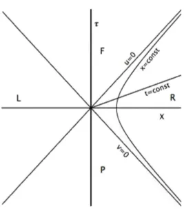
Some comments are now in order. First of all, we notice that a translation in the coordinate t, with x fixed, corresponds to a homogeneous Lorentz transformation in the (τ, X) space: this is the reason why the metric of flat space has an explicit static form with respect to the curvilinear coordinates (t, x). Then, it is easy to see that the classical Cauchy problem should be well posed for initial conditions on any hypersurface t = const. Secondly, tajectories with x = const are hyperbolae and therefore represent the world lines of a uniformly accelerated observer (see Figure 2.1). In order to under-stand better the meaning of this coordinate system, let us write (x, t) in a slight different way (that is often used in many texts): namely
τ = e aξ a sinh(aη) (2.33) X = e aξ a cosh(aη) (2.34) with −∞ < η, ξ < ∞; the line element becomes
Figure 2.1: Rindler coordinates in Minkowski space: both in R and L lines with con-stant t are straight lines through the origin, while lines with x = const are hyperbolae representing uniformly accelerated observers, with null asymptotes u = 0, v = 0. The Rindler coordinates are non-analytic across u = 0 and v = 0: the four regions R, L, F, P must be covered by separate coordinate patches.
from which we can see that it is a conformal transformation of the Minkowski metric. Of course, the coordinates (η, ξ) still cover the same region MR of
the Minkowski spacetime as (t, x). We can see as before that lines with constant η are straight, X ∝ τ, while lines of constant ξ are hyperbolae, X2 − τ2 = a−2e2aξ = const, where ae−aξ is the proper acceleration. Thus,
lines of large positive ξ, i.e. far from X = τ = 0, represent weakly accelerated observers, while the hyperbolae that approach X = τ = 0 carry a high proper acceleration. It should be noticed that all the hyperbolae are asymptotically null, that is, approach the null rays (let us call them as u = 0, v = 0) of the light cone of the Minkowski space: the accelerated observers get close to the speed of light as η → ±∞. Therefore, it is easily understood that the causal structure of the Rindler wedge is not trivial. The Rindler observers approach, but do not cross the null rays u = 0, v = 0 : these, then, act as event horizons and the two regions MR and ML are causally disjoint.
No event from the region of the Minkowski spacetime beyond the null rays can be witnessed by the Rindler observers, neither can causally influence them. This can also be seen in the Penrose conformal diagram below (Figure 2.2), where timelike lines with x = const do not intersect the vertices i± as they do in the Minkowski space, but the lower ones. Thus, for instance, the upper null ray acts as a future horizon and events in the portion marked F cannot causally influence the diamond shaped R region. Moreover, we
notice that a three-dimensional hypersurface with t = const describes events that are simultaneous from the point of view of the accelerated observers. This surface is a hyperplane with constant ratio τ /X. All such hyperplanes cross one another at τ = X = 0, and therefore it is evident that the proper distance between world lines of Rindler observers is time indipendent, and thus the Rindler frame is rigid. Finally, we notice that, in order for the frame to be rigid, two trajectories of the family with different values of X must have different accelerations at a given moment of time τ ; this means that the larger is the value of X, the smaller is the acceleration.
Figure 2.2: Penrose conformal diagram of Rindler system. Timelike lines with x = const do not intersect i± as they do in Minkowski space: events in F cannot be witnessed in R,
2.2
Scalar Field in a Rindler Space
As a first example, let us consider the quantization of the Scalar Field in the right Rindler wedge MR, as the results achieved here will be useful for the
study of the quantization of the Vector Field that we are going to explore in the next chapter.
We start with the Lagrangian density
L(x) = 1 2[−g(x)] −1 2 �gµν(x) φ(x) ,µφ(x),ν− m2φ(x)2 � (2.36)
whose equations of motion are
(gµν(x)∇µ∂ν + m2) φ(x) = 0 (2.37)
that can be explicitly rewritten as � 1 a2x2 ∂ ∂t2 − ∆ − 1 x ∂ ∂x + m 2 � φ(t, x, y, z) = 0 (2.38)
where ∆ is the Laplace operator. In order to find the solution, it is useful to introduce the partial Fourier Transform, given by
φ(t, x, y, z) = � +∞ −∞ dE √ 2π � d2k ⊥ 2π φ(E, k˜ ⊥, x) e −iEt+ik⊥·x⊥ (2.39) where x⊥ = (y, z), k⊥ = (ky, kz) (2.40)
so that the equation (2.38) simplifies in � d2 dx2 + 1 x d dx + E2 a2x2 − (m 2+ k2 ⊥) � ˜ φ(x, E, k⊥) = 0 (2.41) the solutions of which are expressed in terms of Bessel functions of imaginary order, i.e.
˜
φ(x, E, k⊥) = c1(E, k⊥) Iiα(b x) + c2(E, k⊥) Kiα(b x) (2.42)
where α = E a, b = � m2+ k2 ⊥ (2.43)
However, the solutions Iiα(b x) are usually rejected since they are
are thus left with the normal modes decomposition of the real Scalar Field in the right Rindler wedge: namely,
φ(t, x, y, z) = � +∞ −∞ dE √ 2π � d2k ⊥ 2π �
f (E, k⊥) Kiα(b x) e−iEt+ik⊥·x⊥+ c.c.
� (2.44) where the reality conditions
f (−E, −k⊥) = f∗(E, k⊥) (2.45) and the property Kiα(b x) = K−iα(b x) are to be taken suitably into account.
We can now introduce an invariant inner product between any two solu-tions of the covariant Klein-Gordon equation (2.38) of the form
(φ1, φ2)≡
�
Σ
φ∗1(x) i←∂→λ φ2(x) dΣλ (2.46)
In particular, as a Cauchy hypersurface, let us consider the initial time three dimensional hypersurface with
dΣ0 =− 1
a xθ(x) dx d
2x
⊥ dΣi = 0, i = 1, 2, 3 (2.47)
A complete orthonormal set of positive frequency solutions of eq. (2.38) is then given by the generalization of the so called Fulling modes:
˜ ϕE,k⊥(x) = θ(x) 2 π2√a � sinh � πE a � Kiα(b x) e−iEt+ik⊥·x⊥ (2.48)
where the normalization constant can be fixed e.g. by the requirement ( ˜ϕE,k⊥, ˜ϕE�,k�
⊥) = δ(E− E
�) δ(2)(k
⊥− k⊥� ) (2.49)
This way, our invariant scalar normal modes have standard canonical dimensions [ ˜ϕE,k⊥] = cm1/2 in natural units. We can therefore expand the
scalar field φ(x) in terms of these modes and proceed to the quantization, obtaining φ(x) = � +∞ −∞ dE � d2k⊥ �
aE,k⊥ϕ˜E,k⊥(x) + a†E,k⊥ϕ˜∗E,k⊥(x)
�
(2.50)
where the operators a, a† satisfy the following commutation relations
� aE,k⊥, a†E�,k� ⊥ � = δ(E− E�) δ(2)(k⊥− k⊥� ) (2.51) � aE,k⊥, aE�,k� ⊥ � = 0 (2.52) � a†E,k⊥, a†E�,k� ⊥ � = 0 (2.53) ∀k⊥, k⊥� ∈ 2 and ∀E, E� ∈ (2.54)
and have canonical dimensions [a] = cm3/2 in natural units. It should be
noticed that the spinless and chargeless quanta
a†E,k⊥|0� (E, k⊥ ∈ 3) (2.55)
correspond to pseudoparticles, with indefinite energy E ∈ , but fixed trans-verse wave numbers k⊥∈ 2. Clearly, the same would be true for the
multi-pseudoparticles completely symmetric states. 1
1An explicit calculation of the Bogolyubov coefficients and the rigorous check of the
Chapter 3
Vector Fields in a Rindler
Space
In this chapter we will focus on the quantization of the Vector Field, both massive and massless, in the right Rindler wedge MR. We will consider two
gauges in particular, that is the Feynman gauge and the axial gauge, as they appear to be the most interesting ones in this contest.
Before starting, we would like to point out that in our metric the following properties hold true, namely
Fµν = ∇µAν − ∇νAµ = ∂µAν− ΓλνµAλ− ∂νAµ+ ΓλµνAλ = ∂µAν− ∂νAµ (3.1) while Fµν = gρµgσνFρσ = gρµgσν(∂ρAσ − ∂σAρ) = gρµ∇ ρgσνAσ+ gρµgσνΓλσρAλ− gσν∇σgρµAρ− gρµgσνΓλρσAλ = ∇µAν − ∇νAµ = gµρ∇ρAν − gνρ∇ρAµ = gµρ(∂ρAν + ΓνρλAλ)− gνρ(∂ρAµ+ ΓµρλAλ) = ∂µAν − ∂νAµ+ gµρΓν ρλAλ − gνρΓ µ ρλAλ (3.2)
and in particular, by taking two covariant derivatives of the field strenght tensor one gets
∇ν∇µFµν =
� ∂νΓµµλ
�
Moreover, since the Rindler spacetime is flat, one obtains
[∇µ, ∇ν] Aρ =−Rλµνρ Aλ = 0 (3.4)
3.1
Quantization of the Vector Field in the
Feynman gauge
Consider the Vector Field in the space-like regionMR: it is described by the
Lagrangian density L =√−g � −1 4Fµν(x)F µν(x) + 1 2m 2A µ(x) Aµ(x) + Aµ(x) ∂µB + 1 2ξ B 2(x) � (3.5) which leads to the equations of motion for Aν and B, namely
∇µFµν(x) + m2Aν(x) + ∂νB(x) = 0 (3.6)
∇µAµ(x) = ξ B(x) (3.7)
These equations can be simplified choosing the Feynman gauge ξ = 1, so that they become
∇µFµν(x) + m2Aν(x) + ∂νB(x) = 0 (3.8)
∇νAν(x) = ∂νAν(x) + ΓννλAλ(x) = B(x) (3.9)
(∇µ∂µ+ m2)B(x) = 0 (3.10)
which can be explicitly written in the form � 1 a2x2 ∂ 2 t − ∆ + m2− 3 x∂1 � A0(x) = − 2 a2x3 ∂0A 1(x) (3.11) � 1 a2x2 ∂ 2 t − ∆ + m2− 1 x∂1+ 1 x2 � A1(x) = −2 x ∂0A 0(x) (3.12) � 1 a2x2 ∂ 2 t − ∆ + m2− 1 x∂1 � A⊥(x) = 0 (3.13) and � 1 a2x2 ∂ 2 t − ∆ + m2− 1 x∂1 � B(x) = 0 (3.14)
In particular, considering the second equation (3.12), if we sobstitute the transversality condition (3.9),
∂0A0(x) = B(x)− ∂1A1(x)− ∂⊥· A⊥(x)−
1 xA
the equation can be recast as � 1 a2x2 ∂ 2 t − ∆ + m2− 3 x∂1− 1 x2 � A1(x) = −2 x � B(x)− ∂⊥· A⊥(x)� (3.16)
Now, in order to find the solutions, it is convenient to introduce the partial Fourier Transform for Aµ and B given by
Aµ(t, x, y, z) = � +∞ −∞ dk0 √ 2π � d2k ⊥ 2π A˜ µ(k 0, k⊥, x) e−ik0t+ik⊥·x⊥ (3.17) B(t, x, y, z) = � +∞ −∞ dk0 √ 2π � d2k ⊥ 2π B(k˜ 0, k⊥, x) e −ik0t+ik⊥·x⊥ (3.18)
In fact, this way the equations simplify, obtaining � d2 dx2 + 1 x d dx + k2 0 a2x2 − (m 2+ k2 ⊥) � ˜ B(x, k0, k⊥) = 0 (3.19) � d2 dx2 + 1 x d dx + k2 0 a2x2 − (m 2+ k2 ⊥) � ˜ A⊥(x, k0, k⊥) = 0 (3.20) � d2 dx2 + 3 x d dx + k2 0 a2x2 − (m 2+ k2 ⊥) � ˜ A0(x, k0, k⊥) =− 2 a2x3 i k0A˜ 1 (3.21) � d2 dx2 + 3 x d dx + 1 x2 � k2 0 a2 + 1 � − (m2+ k2 ⊥) � ˜ A1(x, k0, k⊥) = 2 x( ˜B − i k⊥· ˜A ⊥) (3.22)
Now we see that the equations for ˜B and ˜A⊥ are just the same as the ones
obtained for the Scalar Field (see 2.41), so that we can immediatly write down the solutions for the real transverse vector field and the auxiliary field in terms of the normal modes, namely
B(t, x, y, z) = � +∞ −∞ dk0 √ 2π � d2k ⊥ 2π �
f (k0, k⊥) Kiα(b x) e−ik0t+ik⊥·x⊥+ c.c.
� A⊥(t, x, y, z) = � +∞ −∞ dk0 √ 2π � d2k ⊥ 2π �
f⊥(k0, k⊥) Kiα(b x) e−ik0t+ik⊥·x⊥+ c.c.
� (3.23) where again the reality conditions
f⊥(−k0,−k⊥) = f⊥∗(k0, k⊥) and f (−k0,−k⊥) = f∗(k0, k⊥) (3.24)
and the property Kiα(bx) = K−iα(bx) are to be taken suitably into account.
˜
A1 first: the solution of the equation (3.22) is the sum of the homogeneous
solution and of the inhomogeneous one. For what concerns the homogeneous equation, we see that it is a special case of the general differential equation
x2y��(x) + (1− 2s) x y�(x) +��s2− r2ν2�+ a2r2x2r�y(x) = 0 (3.25)
whose most general solutions are of the form
y(x) = (±x)sZ
ν(± a xr) (3.26)
where Zν is a Bessel function of any kind: in our case we have to set
s =−1, r = 1, a = i b, ν = i α = i k0/a
so that, if we write ˜
A1(x, k0, k⊥) = ˜V1(x, k0, k⊥) + ˜I1(x, k0, k⊥) (3.27)
where ˜V1 is the solution of the homogeneous equation, we have
˜
V1(x, k0, k⊥) = f1(k0, k⊥)
Kiα(b x)
x (3.28)
while we can obtain the solution ˜I1 through the Green function G(x, x�)
which satisfies the differential equation � x2 d 2 dx2 + 3 x d dx + k2 0 a2 + 1− x 2(m2+ k2 ⊥) � G(x, x�) = δ(x− x�) (3.29) By writing G(x, x�) in the form
G(x, x�) = c1(x�) θ(x− x�) Kiα(b x) x + c2(x �) θ(x�− x)Iiα(b x) x (3.30) one obtains G(x, x�) = 1 b x x� θ(x− x�) I
iα(b x�)Kiα(b x) + θ(x�− x) Kiα(b x�) Iiα(b x)
K�
iα(b x�) Iiα(b x�)− Iiα� (b x�) Kiα(b x�)
(3.31) Thus, we have ˜ I1(x, k0, k⊥) = � ∞ 0 dx�2 x�G(x, x�) ( ˜B(x�, k0, k⊥)− i k⊥· ˜A⊥(x�, k0, k⊥)) (3.32)
In order to evaluate this expression at least asymptotically, we recall the expansion of the Bessel functions given by
Iν(z) ∼ ez √ 2πz � 1− 1 2 z Γ(ν + 32) Γ(ν− 12) +· · · � (3.33) Kν(z) ∼ � π 2ze −z � 1 + 1 2 z Γ(ν + 32) Γ(ν −1 2) +· · · � (3.34) Iν�(z) = 1 2 [Iν+1(z) + Iν−1(z)] ∼ e z √ 2πz � 1− 1 4 z � Γ(ν + 52) Γ(ν + 12) + Γ(ν + 12) Γ(ν − 3 2) � +· · · � (3.35) Kν�(z) = −1 2 [Kν+1(z) + Kν−1(z)] ∼ � π 2ze −z � 1 + 1 4 z � Γ(ν + 52) Γ(ν + 12)+ Γ(ν + 12) Γ(ν− 3 2) � +· · · � (3.36)
Now we can get for the leading behaviour
Kν(z) Iν�(z) ∼ 1 2 z � 1− 1 4 z � Γ(ν + 5 2) Γ(ν + 1 2) + Γ(ν + 1 2) Γ(ν− 3 2) − 2Γ(ν + 3 2) Γ(ν − 1 2) � +· · · � −Iν(z) Kν�(z) ∼ 1 2 z � 1 + 1 4 z �Γ(ν + 5 2) Γ(ν + 1 2) + Γ(ν + 1 2) Γ(ν − 3 2) − 2Γ(ν + 3 2) Γ(ν −1 2) � +· · · �
so that, for large x and x� we have
b−1[Kiα� (b x�) Iiα(b x�)− Iiα� (b x�) Kiα(b x�)]−1 ≈ −x� (3.37)
G(x, x�)≈ 1 2 b x −1 √ x x� � θ(x− x�) ex�−x+ θ(x� − x) ex−x�� (3.38) Then, the integral in (3.32) is well definite and convergent, although it can-not be expressed in closed form. However, this will can-not be a problem, as we shall see in the next section.
3.1.1
Polarization Vectors
In order to introduce properly the polarization vectors, it is useful to consider a particular solution of the field equation with
Actually, this choice enables us to decompose the vector field Aµ only in
terms of the homogeneous solutions of the equations (3.20 - 3.22): namely, ˜ A⊥(x, k0, k⊥)≡ ˜V⊥(x, k0, k⊥) (3.40) ˜ A1(x, k0, k⊥) = ˜V1(x, k0, k⊥) (3.41) ˜ A0(x, k0, k⊥) = ˜V0(x, k0, k⊥) =− i k0 � d dx + 1 x � ˜ V1(x, k0, k⊥)(3.42)
and equation (3.15) reduces to
∂tV0+ � ∂x+ 1 x � V1 = 0 (3.43) which involves only the two components V0 and V1. We can then write the
components of the vector field in terms of normal modes of the Fulling type, i.e.
˜
ϕ⊥E, k⊥(x) = f⊥(E, k⊥) Kiα(b x) e−iEt+ik⊥·x⊥ (3.44)
˜ ϕ1E, k⊥(x) = f1(E, k⊥)Kiα(b x) x e −iEt+ik⊥·x⊥ (3.45) ˜ ϕ0E, k⊥(x) = − i Ef 1(E, k ⊥) b K� iα(b x) x e −iEt+ik⊥·x⊥ (3.46)
We are now ready to define the inner product between any two solutions φµ
r(x) of equations (3.8, 3.9). We proceed as follows: if we consider the
covariant vector current
Jλ(x) = gµν(x) φµr∗(x) i
←→
∇λφνs(x) (3.47)
we can immediatly verify that, thanks to the equations of motion satisfied by φµ
r(x), it is covariantly conserved, i.e. ∇λJλ = 0. Thus we can define the
product
(φµr, φνs) = �
Σ
dΣλφµr∗(x) i gµν(x)∇←→λφνs(x) (3.48)
which is a straightforward generalization of the scalar inner product (2.5); in particular, we will consider the initial time three dimensional hypersurface with
dΣ0 =− 1
a xθ(x) dx d
2x
so that (3.48) becomes ( φνs, φµr) = � Σ dΣ0gµν(x) φν∗s (x) i ↔ ∇0φµr(x) = 1 a � d2x⊥ � ∞ 0 dx x gµν(x) � − φν∗s (x) i ↔ ∂tφµr(x) + i Γν 0ρ(x) [ φµ∗s (x) φρr(x)− φρ∗s (x) φµr(x) ] � = 1 a � d2x⊥ � ∞ 0 dx � 1 x φ ∗ s(x) i ↔ ∂tφr(x) − a2x φ0∗ s (x) i ↔ ∂tφ0r(x) − 2i a2�φ1∗ s (x) φ0r(x)− φ0∗s (x) φ1r(x) � �
In order to compute explicitly the above inner product, it is convenient to introduce the following orthogonal controvariant vectors
e01(x, E, k⊥) = − i E xK � iα(b x) e11(x, E, k⊥) = 1 b x Kiα(b x), e ⊥ 1(x, E, k⊥) = 0 (3.50) eµ2(x, E, k⊥) = Kiα(b x) δµ2, e µ 3(x, E, k⊥) = Kiα(b x) δ3µ (3.51)
which clearly satisfy
gµν(x) eµr(x, E, k⊥) eνs(x, E, k⊥) = 0 for r�= s, r, s = 1, 2, 3 (3.52)
the first one representing a longitudinal polarization along the acceleration axis, while the other two being transverse polarizations, orthogonal to each other and to the direction of the acceleration. We can thus build up the vector analogues of the Fulling scalar normal modes, i.e.
uµE, k
⊥, r(x) =Nre
µ
r(x, E, k⊥) e−iEt+ik⊥·x⊥ (3.53)
where Nr are real normalization constants to be suitable defined. Owing to
(3.52), these vector normal modes are orthogonal to each other:
gµν(x) uµE, k⊥, r(x) uνE, k⊥, s(x) = 0 for r�= s, r, s = 1, 2, 3 (3.54)
For the transverse polarizations, the normalization constants Nr can be set
considering the inner product � ujα�, k� ⊥, r(x), u j α, k⊥, r(x) � = � d2x⊥ � ∞ 0 dx axu j r, α�, k⊥(x) ←→ ∂0 ujs, α�, k� ⊥(x) = (2π)2δ2(k⊥− k� ⊥) (α + α�) e−ia(α−α �)t N2 r � ∞ 0 dx axKiα�(bx) Kiα(bx) = (2π)2δ(2)(k⊥− k⊥� )Nr2π2csch(−πα) δ(α − α�) (3.55)
so that we can define
Nr =
�
sinh (πE/a)
2√a π2 (3.56)
and thus the normal modes become
uµE, k ⊥, r(x) = � sinh (πE/a) 2√a π2 Kiα(bx) δ µ r e−iEt+ik⊥·x⊥ r = 2, 3 (3.57)
which, as expected, have the same form as the normal modes obtained for the scalar field, since the equations satisfied by both are the same. It should be noticed also that these normal modes have canonical dimensions [uµE, k
⊥, r] =
cm1/2 in natural units, as they have in the usual Minkowski space, while now
satisfy � Σ dΣλuµ∗E�, k� ⊥, r(x) i gµν(x) ←→ ∇λuνE, k⊥, s(x) = a−1δ(2)(k⊥− k�⊥) δ(α− α�) (3.58) Instead, for what concerns the longitudinal normal modes, the inner product turns out to be a little bit more complicated, since in our metric the covariant derivative involves directly these modes. We have
� Σ dΣλgµν(x) uEµ∗�, k� ⊥, 1(x) i ↔ ∇λuE, kν ⊥, 1(x) = 1 a � d2x⊥ � ∞ 0 dx � 1 x u 1∗ E�, k� ⊥, 1(x) i ↔ ∂tuE, k1 ⊥, 1(x) − a2x u0∗ E�, k� ⊥, 1(x) i ↔ ∂tuE, k0 ⊥, 1(x) − 2i a2�uE1∗�, k� ⊥, 1(x) u 0 E, k⊥, 1(x)− uE0∗�, k� ⊥, 1(x) u 1 E, k⊥, 1(x) � � = (2π)2δ(2)(k⊥− k� ⊥)N12 � ∞ 0 dx x I(α, α �; bx) e− it(E−E�) (3.59)
where we have set
I(α, α�; ζ) ≡ � α + α� ζ2 Kiα�(ζ) Kiα(ζ)− α + α� αα� K � iα�(ζ) Kiα� (ζ) − 2 ζ � Kiα�(ζ) Kiα� (ζ) 1 α + 1 α� K � iα�(ζ) Kiα(ζ) �� (3.60)
with ζ = b x . Notice that the integrand I(α, α�; ζ) is even under the exchange
and evaluated thanks to the analytic continuation (see Appendix A). This way, the inner product between the longitudinal normal modes gives
� Σ dΣλgµν(x) uEµ∗�, k� ⊥, 1(x) i ↔ ∇λuE, kν ⊥, 1(x) = (2π)2δ(k⊥− k⊥� )N12 � ∞ 0 dx x I(α, α �; bx) e− it(E−E�) = (2π)2δ(2)(k⊥− k⊥� )N12 π2 α2 csch(− πα) δ(α − α �) (3.61)
and we can set
N1 =
α 2π2
�
a−1sinh(πα) (3.62)
We are thus left with a complete orthonormal set of normal modes of the Fulling-type, with three indipendent polarizations, i.e.
uα, kµ ⊥, r(x) = 1 2π2 � a−1sinh(πα) eµ r(α, k⊥; x) ei k· x−i a α t (x > 0) r = 1, 2, 3 α = E/a∈ k⊥ ∈ 2 b = � k2 ⊥+ m2 (3.63) with eµ1(α, k⊥; x) = 1 x �α b Kiα(bx) δ µ 1 + i 2a[ Kiα−1(bx) + Kiα+1(bx) ] δ µ 0 � (3.64) eµr(α, k⊥; x) = Kiα(bx) δrµ r = 2, 3 (3.65)
which fulfil the orthonormality relations
− � Σ dΣλgµν(x) uEµ∗�, k� ⊥, 1(x) i ↔ ∇λuE, kν ⊥, 1(x) = a−1δ(2)(k⊥− k� ⊥) δ(α− α�) δrr� (3.66)
together with the reduced Lorenz condition
∂0uα, k0 ⊥, r(x) + � d dx+ 1 x � uα, k1 α, r(x) = 0 (3.67) α∈ k⊥ ∈ 2 r = 1, 2, 3
Notice that the normal modes have canonical dimensions [ uα, kµ
⊥, r] =
√ cm , in natural units, just like the Fulling scalar functions (2.48) and their usual Minkowski counterparts (1.28).
3.1.2
Canonical Quantization
We can now write the Vector and the auxiliary fields in terms of the normal modes solutions just found, namely,
Vµ(x) = � α, k⊥, r � fα, k⊥, ruα, kµ ⊥, r(x) + fα, k∗ ⊥, ruα, kµ∗⊥, r(x) � (3.68) B(x) = a� α, k⊥ � bα, k⊥uα, k⊥(x) + b∗α, k⊥uα, k∗ ⊥(x) � (3.69)
where we have introduced the shorthand notations � α, k⊥, r ≡ a � ∞ −∞ dα � d2k ⊥ 3 � r=1 � α, k⊥ ≡ a � ∞ −∞ dα � d2k ⊥ (3.70)
fα, k⊥, r and bα, k⊥ being complex coefficients. The general solutions of the
field equations (3.6, 3.7) are then given by
Aµ(x) = Vµ(x) + ∆ Aµ(x) (3.71) ∆ A2(x) = ∆ A3(x) = 0 (3.72) ∆ A1(x) = 2 δ1µ � ∞ −∞ dx�x� G(x, x�) B(t, x�, x⊥) (3.73) ∆ A0(x) = 2δ0µ � ∞ −∞ dα iα e −i a α t × �� d dx + 1 x � � ∞ −∞ dx�x� G(x, x�) �B(α, x�, x⊥)−12B(α, x, x� ⊥) � (3.74) B(x) = B(x)− ∂⊥· V⊥(x) = a � ∞ −∞ dα e−i a α t B(α, x, x� ⊥) (3.75) We can then proceed to the canonical quantization by replacing the classical field functions with the corrisponding operator valued distributions
Vµ(x) = � α, k⊥, r � fα,k⊥,ruα,kµ ⊥,r(x) + fα,k† ⊥,ru µ∗ α,k⊥,r(x) � (3.76) B(x) = a� α, k⊥ � bα, k⊥uα,k⊥(x) + b†α, k⊥uα,k∗ ⊥(x) � (3.77)
which satisfy the canonical commutation relations [ fα, k⊥, r, fα†�, k� ⊥, r�] = a −1δ(2)(k ⊥− k⊥� ) δ(α− α�) δrr� (3.78) [ fα, k⊥, r, fα�, k� ⊥, r�] = [ f † α, k⊥, r, fα†�, k� ⊥, r�] = 0 (3.79)