5 - Simulation Scenario
5.1 - The Network Simulator NS2
As said in the introduction, NS2 is a discrete event simulator widely accepted and used for the analysis of the computer networks. NS2 is free and open-source. This means that everybody can modify the program by inserting new characteristics or by fixing some bugs (that still are found today) [Manual]. The Information Science Institute makes the whole package available in their site www.isi.edu [isi]. We have used version 2.1b8a all-in-one for Linux, with the addition of the MSNv2 patch to simulate the Multiprotocol Label Switching features [isi].
The VINT Project treats the developing of the NS2 official release, it is a project collaboration of UC Berkeley, LBL, USC/ISI and Xerox PARC, that is supported by DARPA (Defense Advanced Research Projects Agency).
NS2 is an object oriented simulator, written in C++, with an OTcl (Object Tool Command Language) interpreter, an Object-oriented version of Tcl, as a front-end. This architecture allows a great personalization as regards the simulation routines at a level of software package (implemented in C++), and an easy tuning and flexible control of the simulation using a simple language, as the OTCL.
In particular OTcl is used:
• for setup, configuration, “one-time” actions
• if is possible to do what is needed by manipulating the existing C++ objects (avoiding the creation of new ones)
• doing anything that requires processing each packet of a flow
• needed to change the behavior of an existing C++ class in ways that were not anticipated, or creating a new C++ class
In a simulation, every real component must be associated to a virtual object that can mirror its characteristics. OTcl provides the interface used by users to describe the model of simulation, to specify the topology of the network, that is the number of nodes and their interconnections, the applications that produce traffic, the instants in which they activate and they stop, etc.
NS2 is able to support a great number of protocols:
• Almost all variants of TCP and UDP
• Routing Protocol:
Unicast, Multicast, and Hierarchical Routing etc.
• Wired Networking :
LAN, MPLS, Diff-Serv/Int-Serv, Scheduling or queue management in routers, and Multimedia Communication etc.
• Mobile Networking:
Pure Wireless LAN and Mobile Ad-Hoc network. Mobile IP Extension to the Wireless Model.
• Satellite Networking Routing and Handoff etc.
• Emulation
In addition to these, there are lots of contributed/additional protocols not in the main distribution as NS2 represents also a rich infrastructure to develop new protocols. [Manual]
NS2 is not a polished and finished product, but the result of an on-going effort of research and development, so that everybody can modify the program by inserting new characteristics or by fixing some bugs (that still are found today) [Manual]. For this reason it is important that whoever is using NS knows that has to verify by himself the correctness and the reliability of the simulations, because it is possible that they could be affected by errors.
According to what is specified in the input script, NS2 can produce as output different kinds of trace files that may be provided as input to programs like Nam, the Network Animator, or may be used (as text files) to do an accurate analysis of the parameters in the simulation we want to do. The default NS2 trace file contains information concerning the typology of the net (nodes and connections), the simulation events, and the packets that have moved in the network [Garroppo, 03] [Manual].
In the simulations a patch to insert a time stamp field in the packet header has been used for the results analysis, so that, through the study of many text files printed by NS2, was possible the monitoring of:
• Throughput
• Delay
• Jitter
Those are fundamental parameters to grant a good level of quality of service, in particular as regards the audio-video traffic, where every loss is an imperfection. Another fundamental parameter monitored for UDP is:
• Packet Loss
All the results have been put in Excel XP (Microsoft) for a deeper analysis and to create the graphs.
5.1.1 - The MNSv2 patch
NS2 has been integrated with the MNSv2 patch. The MPLS Network Simulator (MNS) has been developed to extend the NS2 capabilities with the primary purpose of developing a simulator that enables to simulate various MPLS applications without constructing a real MPLS network.
This patch gives to the simulator a good support to the establishment of CR-LSP (Constraint based Routing-Label Switching Path) for QoS traffic as well as basic MPLS functions as LDP (Label Distribution Protocol) and label switching. MNS consists of many components, CR-LDP, MPLS Classifier, Service Classifier, Admission Control, Resource Manager and Packet Scheduler (as shown in figure 5.1).
All the components added by the MNS patch have been used in these simulations to give to NS2 a good level of QoS, with the adding of a Weighted Round Robin scheduling mechanism.
5.2 Network Architecture
The simulation has been made for the purpose of studying the response of a highly redundant 12 nodes MPLS network core (blue nodes in figure 5.2) to a classified traffic that may exceed the capacity of a single link by nine times, granting a high differentiated level of QoS. It was specified that the network core should have at least 5 link-disjoint paths (i.e. without common links) between each pair of nodes (i.e., the network core is 5-connected).
To generate the network core, the method of Steiglitz has been used. The basic idea is to use the theorem of Whitney. If we need a k-connected network, we have to ensure that every node has at least k links. This is a not sufficient, but necessary condition.
We start by numbering the nodes randomly. Then a link deficit number is associated to every node, that is equal to the number of links still necessary to that node. In our case, five links.
The Steiglitz method then proceeds by adding links one at a time until the deficit at each node is zero or less. To add a link XY, X and Y are chosen in the following way [Tanenbaum, 81]:
• X: find the node with the highest deficit. In the case of a tie, choose the node with the lowest number.
• Y: find the node not already adjacent to X with the highest deficit. In case of a tie choose the node whose distance from X is the minimum. If several nodes are at the same distance, take the one with the lowest number.
Finally, it was verified that the network obtained by the Steiglitz method had indeed at least 5 link-disjoint paths between each pair of nodes, so no further modification was necessary.
The red nodes in figure 5.2 are edge routers where the traffic sources and traffic destinations are placed.
We want to simulate a DiffServ MPLS network, so in each simulation (except the first, because it is without QoS), the traffic is divided into three traffic classes: Gold, Silver and Bronze (Bronze is treated as the best-effort traffic, so beginning from now the two terms will be used indifferently).
Two traffic types will be used in the simulations representing two usual Internet applications: FTP (over TCP Reno) and Constant-bit-rate to simulate VoIP phone calls (over UDP).
11
7
0
10
9
2
5
6
8
3
4
1
14
13
12
16
17
15
Figure 5.2 – Network topologyThere is a Service Level Agreement (SLA) between the ISP and the customers; the objective is to obtain different treatments for the aggregated flows according with their traffic class. The target of this work is to compare three different scenarios. The SLA is one of the things that varies for each scenario, together with the admission control and the bandwidth assignment.
It is assumed that:
• The capacity of a link in the core (the blue nodes in figure 5.2) is 1000 Kbit/s. The capacity used in the other links is higher and sufficient to support a great amount of traffic, because we are interested to simulate only the network core.
• The delay for each link in the network core is 10ms (1 ms on the other links), that is equivalent to assume the distance between two nodes to be more or less equal to 3000Km, so we are considering a continental scenario.
• The queues in the core links, when we are using MPLS, are Class Based Queue with the support of the Weighted Round Robin (CBQ/WRR). In the no-QoS case it is a simple FIFO with Droptail.
• The bit rate used by a single phone call over UDP is 50Kbit/sec (it is assumed the use of some audio compression algorithm).
• The dimension of a packet is 200 Byte for the UDP and 1000 Byte for TCP; this dimension is fixed for all the sources.
• The case for the VoIP traffic is the worst case, which is: the two phone-callers speak at the same time without any pause (full duplex rate). So the bit rate for a single phone call is 50Kbit/sec in both the directions of a path.
The red nodes in figure 5.2 are edge routers (Label Edge Routers in the MPLS case). They are the border LSR for the MPLS domain, when we use this technology. The reservation required by the SLA starts on the edge routers, where the admission control is performed.
The edge routers have also Bandwidth Broker functions for the dynamic bandwidth assignment in the third scenario.
5.3 - Flows, Common Scenario
A traffic flow consists in a certain number of packets having the same following fields in the network layer header:
< Source IP address; Destination IP address; Protocol ID; Source port; Destination port > MPLS networks are used to forward not single flows, but homogeneous aggregated flows, to avoid scalability problems, staying away from the great amount of information to manage required by a single flow approach. So, it makes sense to define what is an Aggregated Flow (AgF ) in MPLS (that is also called Traffic Trunk) [Tofoni, 03].
An MPLS AgF is directly bound to the concept of LSP Tunnel, which is a Label Switched Path between two egress routers in an MPLS domain (or sub-domain) made to create a virtual connection between those routers. A Traffic Trunk is an aggregation of more single flows passing by the same LSP Tunnel, with some characteristics associated (like QoS, traffic pattern and more) [Tofoni, 03]. In this simulation, to each AgF corresponds an LSP in which the whole traffic has the same:
< Ingress LSR; Egress LSR; Protocol ID; Class of Service>
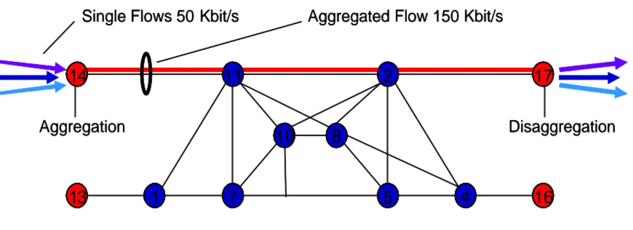
An aggregated bidirectional UDP flow consists in one or more phone calls with the previous characteristics as shown in figure 5.3. To each edge router arrive three AgFs for each class destined to the other three red nodes on the other side of the network, for a total of 9 AgFs directed towards the network core. At the same time each red node is the destination for three AgFs for each class coming from the other side. So we have a total of 54 AgFs for the UDP traffic.
11 7 10 2 5 8 4 1 14 13 16 17 Aggregated Flow 150 Kbit/s
Single Flows 50 Kbit/s
Aggregation Disaggregation 11 7 10 2 5 8 4 1 14 13 16 17 Aggregated Flow 150 Kbit/s
Single Flows 50 Kbit/s
Aggregation Disaggregation
Figure 5.3 – Aggregated flow UDP
Like in the UDP case, in the TCP case three AgFs for each class arrive to each edge router directed to the other three red nodes on the other side of the network, for a total of 9 AgFs (a maximum of 90 single flows, reached only in the simulation with Gold TCP sources and Silver TCP sources fixed to 10) directed towards the network core. Now, the AgFs are unidirectional, directed only from the left edge routers to the right ones for a total of 27 AgFs. The total number of TCP single flows may reach 270, aggregated in groups of maximum 10, as shown in figure 5.4. However, the number of single flows in one AgF varies in the different simulations, randomly in those to analyze the UDP traffic, fixed in those to analyze the TCP traffic.
11 7 10 2 5 8 4 1 14 13 16 17 Aggregated TCP Flow Single TCP Flows (Max 10, min 1)
Aggregation Disaggregation 11 7 10 2 5 8 4 1 14 13 16 17 Aggregated TCP Flow Single TCP Flows (Max 10, min 1)
Aggregation Disaggregation
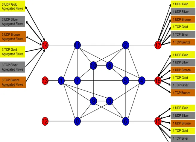
For a better understanding, figure 5.5 gives a good example of the flow distribution for the edge router 14, showing also the destination for the AgFs. UDP traffic is bidirectional. Obviously, to obtain meaningful simulation results, the flow distribution must be the same in the three scenarios.
11
7
0
10
9
2
5
6
8
3
4
1
14
13
12
16
17
15
3 UDP Gold Agregated Flows 3 UDP Silver Agregated Flows 3 UDP Bronze Agregated Flows 3 TCP Gold Agregated Flows 3 TCP Silver Agregated Flows 3 TCP Bronze Agregated Flows 1 UDP Gold 1 UDP Silver 1 UDP Bronze 1 TCP Gold 1 TCP Silver 1 TCP Bronze 1 UDP Gold 1 UDP Silver 1 UDP Bronze 1 TCP Gold 1 TCP Silver 1 TCP Bronze 1 UDP Gold 1 UDP Silver 1 UDP Bronze 1 TCP Gold 1 TCP Silver 1 TCP BronzeFigure 5.5 - Aggregated Flows for edge router 14, and flow destinations
As said before, on the network core is running not a simple Distance Vector Routing Algorithm, but a Constrained Based Routing using the CR-LDP (Constrained based Routing- Label Distribution Protocol) protocol. The algorithm used searches the minimum number of hops and keeps track of the bandwidth available in all the links. Every certain number of seconds (that may be chosen manually), the information about these two parameters, contained in the routers, is refreshed.
When a customer makes its own reservation, the MPLS with its capacity of Traffic Engineering uses the Constrained Based Routing to find a path that can satisfy that reservation, then there is the setting up of a Label Switched Path (LSP), with the assignment of a label to each aggregated flow.
5.4 - First Scenario - No Class Differentiation
The first scenario to be simulated in our network is the simplest one, therefore witho ut any QoS.
So, all the traffic is treated as best-effort and sent on the shortest path.
This scenario is used as basic reference to see the improvements brought by the other two scenarios.
The traffic will be randomly generated (even if many times a higher or lower range of variation for the random generation is given) in the following way for UDP:
• Gold UDP: a random value between 0 Kbit/s and 450 Kbit/s, for each AgF.
• Silver UDP: a random value between 0 Kbit/s and 250 Kbit/s, for each AgF.
• Bronze UDP: a random value between 0 Kbit/s and 50 Kbit/s, for each AgF. So, in each edge router, the UDP total traffic towards the network core is varying between 0 Kbit/s and maximum of 2250 Kbit/s.
While as regards the TCP:
• Gold TCP: a random number of flows, for each AgF, varying between 1 and 10, or a fixed number (from 1 to 10) for the TCP analysis simulations
• Silver TCP: a random number of flows, for each AgF, varying between 1 and 10, or a fixed number (from 1 to 10) for the TCP analysis simulations
• Bronze TCP: a random number of flows, for each AgF, varying between 1 and 10, or a fixed number (from 1 to 10) for the TCP analysis simulations.
As all the traffic is treated as best effort, there is no TE and traffic differentiation, so many links will result overloaded while many others will receive a low level of traffic and a lot of them will be completely unused. As a consequence the results we should obtain in this simulation are a lot of packets lost for every flow (especially for the UDP flows) and really bad values for all the parameters monitored, especially TCP throughput, obtaining really bad values relative to quality of service.
11
7
0
10
9
2
5
6
8
3
4
1
14
13
12
16
17
15
11
7
0
10
9
2
5
6
8
3
4
1
14
13
12
16
17
15
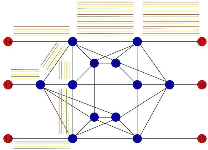
Figure 5.6 – Overcongested link node 11-12
For example, looking at the figure 5.6, it can be noticed that looking only at the traffic directed from the three left LER to node 17, we have an overcongested link between the nodes 11 and 2. The congestion will exist even with just the UDP Gold sources in the cases (that will be simulated) of a heavily loaded network. This can be observed by noting that in this situation of load, the UDP Gold aggregated traffic in the link 11-2 can reach
Obviously the situation is still worse in the case simulated with a number of AgFs considerably greater.
For this reason, a lot of packets will be lost. Besides, it must be remembered that all traffic is treated as best effort, so that the Gold traffic will receive the same treatment and share network resources with the other traffic classes receiving a really high number of losses.
5.5 - Second Scenario - Fixed Bandwidth for each Traffic Class
The second scenario will be simulated using MPLS with Traffic Engineering (TE) together with the Constrained Based Routing commands. An Admission Control will be used for the UDP traffic. The scheduling mechanism used will be the CBQ/WRR (Class Based Queue/Weighted Round Robin).
The Service Level Agreement between the ISP and the customers has been made to obtain particular treatments that are for the UDP:
• A fixed bandwidth reservation, decreasing with the class importance (i.e.: 30% Gold, 15% Silver, and 5% Bronze).
• No packet loss for the Gold and the Silver traffic (if inside their bandwidth reservatio n)
• A very good delay and jitter
The Admission Control is used in the case that one or more AgFs, in one or both the first two classes, are out of the reservations. The behavior in those cases downgrades the selected class as follows:
For the Gold traffic:
o If there is available bandwidth in the Silver class reservation for the AgF that is following the same path than the Gold one (i.e.: the random generation for that AgF in the Silver class is lower than 150 Kbit/s), then
disaggregate the Gold AgF and put the exceeding traffic into a new Silver aggregated flow until the Silver bandwidth reservation is filled. If there is still exceeded bandwidth, then treat that as in the following point.
o If there is no available bandwidth in the Silver class reservation, then disaggregate the Gold AgF and put the exceeding traffic into a new Bronze AgF (i.e.: treat it as best-effort).
For the Silver traffic:
o In both cases, if there is available bandwidth in the Gold class reservation or if there is no available bandwidth in the Gold class reservation, disaggregate the Silver AgF and put the exceeding traffic into a new Bronze AgF. This means that all the exceeded silver traffic is treated as best-effort.
The SLA for the TCP traffic assures:
• A fixed bandwidth reservation, decreasing with the class importance. The FTP throughput is limited (if there is no available bandwidth from other classes aggregated flows on the same path) by the AgF class reservation (i.e.: limited to 30% for Gold and15% for Silver).
• As regard the Best-Effort traffic, there is a small fixed bandwidth (5% of the capacity of each single link) reserved but shared with the Bronze Constant-bit-rate. So all the best-effort traffic reserves only 5 % of the capacity of each single link.
The remaining 5% of the link bandwidth are reserved for the network managing and signaling traffic.
It is important to notice that this second scenario is not just a simple application of the characteristics of the Constrained Based Routing to find a path with an assigned
approach usually taken in not heavily loaded network, were the average link utilization is around 50-60%). Here all the traffic (real time, not real time, UDP, TCP, signaling and managing, and best effort) receives a bandwidth assignment using the same metrics, reserving (with the sum of the assignments) 100% of the capacity of a single link, as explained before. So, the network is always ready to any kind of traffic load, heavily or not heavily loaded, and the treatment given to a traffic class is totally independent of the characteristics of the other traffic classes, obtaining a kind of Protection between the traffic classes.
11
7
10
2
5
8
4
1
14
13
16
17
11
7
10
2
5
8
4
1
14
13
16
17
50 Kbit/s Bronze (best effort) TCP/UDP
Reservation order
150 Kbit/s SIlver TCP 300 Kbit/s Gold TCP 150 Kbit/s Silver UDP 300 Kbit/s Gold UDP
11
7
10
2
5
8
4
1
14
13
16
17
11
7
10
2
5
8
4
1
14
13
16
17
50 Kbit/s Bronze (best effort) TCP/UDP
Reservation order
150 Kbit/s SIlver TCP 300 Kbit/s Gold TCP 150 Kbit/s Silver UDP 300 Kbit/s Gold UDP
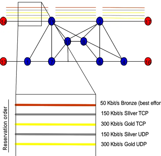
Figure 5.7 – Second scenario reservation example 1
As shown in figure 5.7, the reservation order for is: 1. 300 Kbit/s UDP Gold
3. 300 Kbit/s TCP Gold 4. 150 Kbit/s TCP Silver
5. 50 Kbit/s UDP/TCP Bronze (best effort traffic)
The Silver UDP reservation is made before the TCP Gold to avoid to the Silver UDP longer paths and, as a consequence, worse values as regards the delay and the jitter, parameters not very much important for the TCP traffic but fundamental for the real time UDP traffic. 11 7 10 2 5 8 4 1 14 13 16 17 11 7 10 2 5 8 4 1 14 13 16 17
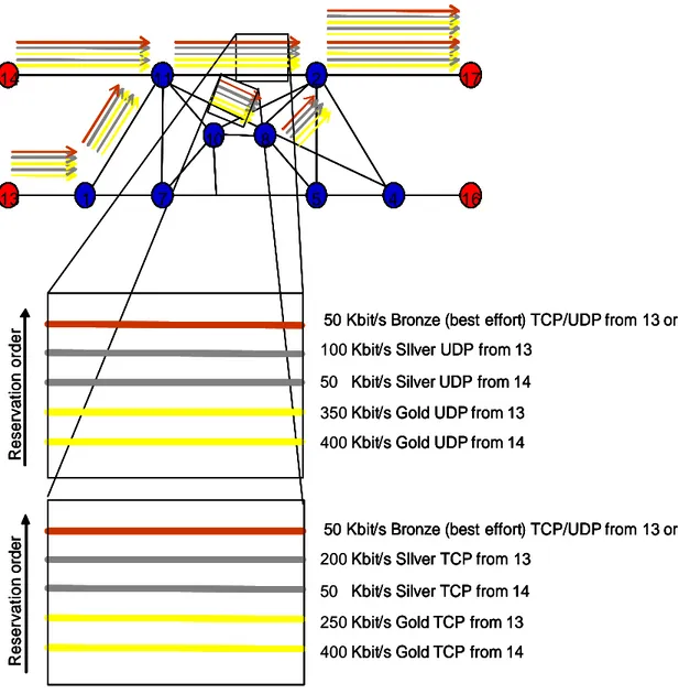
50 Kbit/s Bronze (best effort) TCP/UDP from 13 or 14
Reservation order
150 Kbit/s SIlver UDP from 13 150 Kbit/s Silver UDP from 14 300 Kbit/s Gold UDP from 13 300 Kbit/s Gold UDP from 14
Reservation order
50 Kbit/s Bronze (best effort) TCP/UDP from 13 or 14 150 Kbit/s SIlver TCP from 13
150 Kbit/s Silver TCP from 14 300 Kbit/s Gold TCP from 13 300 Kbit/s Gold TCP from 14 11 7 10 2 5 8 4 1 14 13 16 17 11 7 10 2 5 8 4 1 14 13 16 17
50 Kbit/s Bronze (best effort) TCP/UDP from 13 or 14
Reservation order
150 Kbit/s SIlver UDP from 13 150 Kbit/s Silver UDP from 14 300 Kbit/s Gold UDP from 13 300 Kbit/s Gold UDP from 14
Reservation order
50 Kbit/s Bronze (best effort) TCP/UDP from 13 or 14 150 Kbit/s SIlver TCP from 13
150 Kbit/s Silver TCP from 14 300 Kbit/s Gold TCP from 13 300 Kbit/s Gold TCP from 14
This reservation order starts at the same time for all the flows in the same reservation group. For this reason, many times the reservation path followed by sources belonging to different classes starting at the same LER (Label Edge Router) and arriving at the same LER are different. For a better explanation look at figure 5.8. The TCP traffic, as is reserved after the UDP reservation, follows a different and longer path than the UDP traffic (with just one hop more in this case, but many times the additional hops are not so few).
50 Kbit/s Bronze (best effort) TCP/UDP from 14 or 13 or 12
Reservation order
300 Kbit/s Gold UDP from 12 300 Kbit/s Gold UDP from 13 300 Kbit/s Gold UDP from 14
11
7
0
10
9
2
5
6
8
3
4
1
14
13
12
16
17
15
50 Kbit/s Bronze (best effort) TCP/UDP from 14 or 13 or 12
Reservation order
300 Kbit/s Gold UDP from 12 300 Kbit/s Gold UDP from 13 300 Kbit/s Gold UDP from 14
11
7
0
10
9
2
5
6
8
3
4
1
14
13
12
16
17
15
11
7
0
10
9
2
5
6
8
3
4
1
14
13
12
16
17
15
The reservation, usually, is even more complicated, as can be seen in figure 5.9, where the UDP Gold traffic saturates (with the exception of 50 Kbit/s available for one bronze flow) the capacity of the single link 11-2. As a consequence, all the other traffic follows different paths.
5.5.1 - Objectives of the Second Scenario simulations
To show the improvements that this scenario brought, we will use a heavily loaded traffic pattern, filling the maximum capacity that can be sustained by the network.
In particular we want to show that there is:
• Protection between the different classes (i.e.: excess traffic in one class does not damage the others), as explained in the previous paragraphs.
• A bigger throughput, compared with the first scenario, provided by the network thanks to the use of traffic engineering to find alternative paths.
• Different QoS according to the class selected.
We will show that the objectives prefixed by the SLA will be fully respected. This means that the Gold UDP traffic and the Silver traffic to each node will reach their reservation (respectively 300 Kbit/s and 150Kbit/s, to each destination) receiving a treatment that assures: no packet loss, and a low delay and jitter values according to their class; while Gold and Silver TCP traffic will have an assured throughput by filling the bandwidth available in their reservation (also in this case respectively 300 Kbit/s and 150Kbit/s, to each destination). We don’t care about the Bronze traffic, but the expectations are to have improvements also for this class, due to the use of new alternative paths.
5.6 - Third Scenario – Dynamic Bandwidth for each Traffic Class
The second scenario used fixed bandwidth assignments for each class, which as will be seen can lead to priority inversions when high priority classes are heavily loaded and low priority classes are lightly loaded. An alternative that will be studied in this third scenario is to use dynamic bandwidth for each traffic class according to its traffic load.
The third scenario, like the second one, has to be simulated using MPLS with Traffic Engineering (TE) together with the Constrained Based Ro uting commands. Also here an Admission Control mechanism will be used for the UDP traffic. But, differently from the second scenario, a dynamic bandwidth assignment will be used. The Service Level Agreement for this scenario provides the following treatments:
For the UDP traffic:
• A semi-dynamic bandwidth reservation, decreasing with the class importance (the total amount of the UDP bandwidth for the first two classes is 45% of the capacity of a single link)
• No packet loss for the Gold and the Silver traffic (if inside their bandwidth reservation)
• A very good delay and jitter
The Admission Control now is used in the case that one or more AgFs, in the Silver class, are out of the reservations.
If the Gold is out of the reservation, the Admission Control and Bandwidth Broker will be used as explained in the following:
o If there is available bandwidth in the Silver class reservation for the AgF that is following the same path than the Gold one (i.e.: the random generation for that AgF in the Silver class is lower than 150 Kbit/s), then take that available bandwidth and make a new bandwidth reservation
assigning that available bandwidth to the Gold traffic and assigning to the Silver traffic only the bandwidth effectively used.
If there is still exceeding bandwidth, then treat that as in the following point.
o If there is no available bandwidth in the Silver class reservation, then disaggregate the Gold AgF and put the exceeding traffic into a new Bronze AgF (i.e.: treat it as best-effort).
For the Silver traffic:
o Like in the second scenario, in both the cases, if there is available bandwidth in the Gold class reservation or if there is no available bandwidth in the Gold class reservation, disaggregate the Silver AgF and put the exceeding traffic into a new Bronze AgF. This means that all the exceeding Silver traffic is treated as best-effort.
Why not using the dynamic bandwidth assignation also in the previous case? Because if, for example, a Gold AgF reaches only 100 Kbit/s, a dynamic bandwidth assignment, as explained before, will assign 100 Kbit/s to the Gold and 350 Kbit/s to the Silver. This means that the Gold will receive a worse treatment in the third scenario than in the second scenario (where the default assignment is 300 Kbit/s), giving an excessively good treatment to the Silver traffic (more than the double than the 150 Kbit/s in the second scenario). We want to always give a better treatment for the Gold, because if the Gold pays more, he must receive a better treatment, especially in this case of real time traffic, where a higher bandwidth assignment means a better treatment.
The SLA as regards the TCP traffic assures:
same source node to the same destination node) to receive a bandwidth reservation that is the double of the one received by a single Silver FTP source (the total amount of the FTP bandwidth for the first two classes is 45% of the capacity of a single link).
For each pair of AgFs passing by the same pair of edge routers, the formulas used to grant this assignation are the following:
BG/NG = 2*BS/NS BG + BS = TTCP
Where BG is the Bandwidth to be assigned to a Gold TCP AgF (the number of sources has different values for each AgFs, for this reason also the bandwidth assigned varies for each AgF), BS is the Bandwidth to be assigned to a Silver AgF, TTCP is the total bandwidth that can be used by these two AgFs (i.e.: 450 Kbit/s in this case), NG is the number of Gold sources per aggregated TCP flow, and NS is the number of Silver sources per aggregated TCP flow. Solving the previous equation system we arrive to:
BG = (2*TTCP*NG)/(NS+2*NG)
BS = TTCP - (2*TTCP*NG)/(NS+2*NG)
For a better understanding, let us analyze the case in which there are 8 Gold and 4 Silver TCP sources per AgF. In that case, we have 360 Kbit/s assigned to the Gold TCP AgF, and 90 Kbit/s to the Silver TCP AgF. This assignment leads to an average bandwidth per single Gold TCP flow that is 45 Kbit/s and an average bandwidth per single Silver TCP flow that is 22,5 Kbit/s, exactly one half of the first one, that is what we wanted.
As can be noticed, if the number of Gold and Silver sources is the same, the third scenario gives the same assignments than the second, that is: 300 Kbit/s
• As regards the Best-Effort traffic, there is a small fixed bandwidth (5% of the capacity of a single link) reserved but shared with the UDP.
Also in this scenario there is 5% of the link bandwidth reserved for the network managing and signaling traffic.
11 7 10 2 5 8 4 1 14 13 16 17 11 7 10 2 5 8 4 1 14 13 16 17
50 Kbit/s Bronze (best effort) TCP/UDP from 13 or 14
Reservation
order 100 Kbit/s SIlver UDP from 13
50 Kbit/s Silver UDP from 14 350 Kbit/s Gold UDP from 13 400 Kbit/s Gold UDP from 14
Reservation
order
50 Kbit/s Bronze (best effort) TCP/UDP from 13 or 14 200 Kbit/s SIlver TCP from 13
50 Kbit/s Silver TCP from 14 250 Kbit/s Gold TCP from 13 400 Kbit/s Gold TCP from 14
11 7 10 2 5 8 4 1 14 13 16 17 11 7 10 2 5 8 4 1 14 13 16 17
50 Kbit/s Bronze (best effort) TCP/UDP from 13 or 14
Reservation
order Kbit/s SIlver UDP from 13
Kbit/s Silver UDP from 14 Kbit/s Gold UDP from 13 Kbit/s Gold UDP from 14
Reservation
order
50 Kbit/s Bronze (best effort) TCP/UDP from 13 or 14 Kbit/s SIlver TCP from 13
Kbit/s Silver TCP from 14 Kbit/s Gold TCP from 13 Kbit/s Gold TCP from 14
11 7 10 2 5 8 4 1 14 13 16 17 11 7 10 2 5 8 4 1 14 13 16 17
50 Kbit/s Bronze (best effort) TCP/UDP from 13 or 14
Reservation
order 100 Kbit/s SIlver UDP from 13
50 Kbit/s Silver UDP from 14 350 Kbit/s Gold UDP from 13 400 Kbit/s Gold UDP from 14
Reservation
order
50 Kbit/s Bronze (best effort) TCP/UDP from 13 or 14 200 Kbit/s SIlver TCP from 13
50 Kbit/s Silver TCP from 14 250 Kbit/s Gold TCP from 13 400 Kbit/s Gold TCP from 14
11 7 10 2 5 8 4 1 14 13 16 17 11 7 10 2 5 8 4 1 14 13 16 17
50 Kbit/s Bronze (best effort) TCP/UDP from 13 or 14
Reservation
order Kbit/s SIlver UDP from 13
Kbit/s Silver UDP from 14 Kbit/s Gold UDP from 13 Kbit/s Gold UDP from 14
Reservation
order
50 Kbit/s Bronze (best effort) TCP/UDP from 13 or 14 Kbit/s SIlver TCP from 13
Kbit/s Silver TCP from 14 Kbit/s Gold TCP from 13 Kbit/s Gold TCP from 14
Figure 5.10 – Third scenario reservation example 1
Figure 5.10 represents the simple situation in which there are only traffic flows between node 14 and 17, and between node 13 and 17. In this case there are 8 Gold phone calls from node 14 (400 Kbit/s), 1 Silver calls from the same node (50 Kbit/s), 7 Gold phone
calls from node 13 (350 Kbit/s) and 2 Silver calls from the same node (50 Kbit/s), 8 TCP flows in the Gold AgF from node 14 (400 Kbit/s) and 2 in the Silver AgF from the same node (50 Kbit/s) – it must be remembered that the average bandwidth per single Gold flow must be the double than the Silver one, and not the bandwidth of the AgF, for example, in this case we have an average bandwidth of 50 Kbit/s per Gold TCP flow and 25 Kbit/s per Silver TCP flow -, 5 TCP flows in the Gold AgF from node 13 (250 Kbit/s) and 5 in the Silver AgF from the same node (200 Kbit/s), with the adding of 50 Kbit/s of best effort traffic from both the nodes. In the cases that another Gold UDP try to reserve in the link between node 11 and node 2 after the first two Gold UDP reservations, the link may result with an insufficient bandwidth available (only 200 Kbit/s). This implies that the path assignments can be different between the Second Scenario and the Third, with a consequent difference in the treatments and in the results. This case is represented in figure 5.11, were the third reservation follows another path, different from the one in figure 5.9, with a consequent different assignment of all the paths reserved after that.
11
7
0
10
9
2
5
6
8
3
4
1
14
13
12
16
17
15
400 Kbit/s 350 Kbit/s 300 Kbit/s11
7
0
10
9
2
5
6
8
3
4
1
14
13
12
16
17
15
11
7
0
10
9
2
5
6
8
3
4
1
14
13
12
16
17
15
400 Kbit/s 350 Kbit/s 300 Kbit/s5.6.1 - Objectives of the Third Scenario simulations
With this scenario our target is to illustrate the improvements brought by adding to the second scenario a dynamic bandwidth reassignment, used together with Admission Control. We expect to obtain better results in each field for each traffic type.
This should happen especially as regards the TCP flows.
In order to show this, we will use an overloaded network making different simulations for each one of the following traffic pattern variations:
• First we will vary UDP traffic and leave the TCP fixed to heavily loaded values. o In the beginning, the Gold UDP traffic will be overloaded, showing what
happens to it using respectively overloaded, normal loaded, and under loaded Silver UDP traffic.
• In a second group of simulations we will vary the TCP load leaving the UDP fixed to heavily loaded values. We will vary both the number of Gold and Silver TCP flows, showing the great improvements in this third scenario relative to the second one. For a better understanding of what will happen imagine, for example, in the second scenario, if there were 10 FTP flows on one Gold AgF and only 1 FTP flow on one Silver AgF, then the single Silver flow will occupy (the FTP flows fill the available bandwidth) 150 Kbit/s, while the 10 Gold flows share a bandwidth of 300 Kbit/s, obtaining a single service throughput (an average of 30 Kbit/s) lower than the one obtained by a single flow in the Silver class. The third scenario avoids this priority inversion, assuring a bandwidth reservation per Gold flow that is always the double than the one per Silver flow (here we are speaking about flows and not AgFs).
So, we will vary the proportion between the number of Gold flows and Silver flows (obviously we are speaking about Silver and Gold passing by the same pair
of Label Edge Routers), fixing one to a value and varying the other from 1 TCP source to 10 sources. The objective of this variation is to see the differences between the different patterns and between the two scenarios.