Chapter 4

Chapter 4

Results and discussion

4.1

Characterization of PMAs

4.1.1

Softening Point Test

Softening point increases almost linearly with the quantity of polymer. Results for the tested materials are shown in Figure (4.1). The temperature at which each material was kept during the conditioning time, before testing, was chosen equal to 60°C. This is close to the softening point of PMA S6. It has to be remembered that TR&B is not a melting point; material’s stiffness is gradually lost during the warm up process.

40 45 50 55 60 65 0 1 2 3 4 5 6 [%] SEBS [° C ] T R & B

4.1.2

Penetration Test

Penetration is strongly reduced by the addition of 2% of SEBS. Increasing the quantity of polymer, penetration decreases very slowly, probably reaching some asymptotic value. Results are shown in Figure (4.2).

40 60 80 100 120 140 160 180 200 220 240 0 1 2 3 4 5 6 [%] SEBS [d m m ] P en et ra tio n

Figure (4.2) – Penetration as a function of polymer percentage.

4.1.3

Fluorescence Microscopy

Photos of samples taken during the mixing process and a typical photo of the final blend are shown in Figures (4.3) to (4.10). After 15minutes of mixing, the morphology appeared to be already close to the final one, (independent of the concentration of the polymer). Data and images about high temperature storage stability can be found in [43]; the tuben test was conducted following the European specification (EN 13399). Material S2 and S4 were found to be stable up to the high temperature storage, while S6 showed macroscopic phase separation.

Figure (4.3) – Morphology of S2 after 15min of mixing, 250x.

Figure (4.4) – Final morphology of S2, 250x.

Figure (4.6) – Morphology of S4, after 60min of mixing, 100x.

Figure (4.7) – Final morphology of S4, 250x.

Figure (4.9) – Morphology of S6, after 60min of mixing, 250x.

4.2

Rheological Characterization

4.2.1

Simple Creep

4.2.1.1 Results and discussion

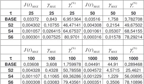
Figure (4.11), page 59, shows the compliance curves for base asphalt and modified asphalt binders obtained from creep and recovery test at 40°C. Applied stress was 25Pa, creep time was 1 minute and recovery time was 9 minutes. The effect of polymer modification was very strong, all modified binders reached very small compliance values in comparison with the base asphalt. The end-of-creep strain, γMAX, was almost eight times smaller for S2 than in the base

asphalt, while for S6 the difference was approximately two orders of magnitude, as reported in Table [4.1], where the ( )J t _MAX and γ_MAX for 25Pa and other applied stresses are shown.

J t( )MAX γMAX (%) r γ J t( )_MAX γ_MAX (%) r γ ττττ 25 25 25 50 50 50 BASE 0,03372 0,843 6,951364 0,03516 1,758 3,782708 S2 0,004302 0,10755 46,47141 0,004308 0,2154 49,67502 S4 0,001057 0,026415 64,67537 0,001061 0,05307 68,54155 S6 0,000301 0,007525 80,9701 0,000316 0,01578 78,29214 ( )_MAX J t γ_MAX (%) r γ J t( )_MAX γ_MAX (%) r γ ττττ 100 100 100 1000 1000 1000 BASE 0,03608 3,608 1,759978 0,04491 44,91 0,289468 S2 0,004328 0,4328 50,78558 0,004572 4,5715 25,4621 S4 0,001107 0,11065 69,36286 0,001229 1,229 56,00895 S6 0,000308 0,03083 79,43561 0,000351 0,3506 78,10896 Table [4.1]

The creep curve for base asphalt approached a straight line very fast. This means that the material starts to flow at a constant shear rate very soon after the stress is applied, i.e. it behaves like a purely viscous fluid. Figure (4.12) is an enlargement of the previous graph. The curvature of J(t) in the creep zone increases (at short times) with the quantity of polymer. As expected, the higher the concentration of polymer, the more pronounced is the delayed elasticity of the modified binder. The percentage of recovered strain (%)

r

γ , defined as

(

)

end of creep

γ γ

γ −

⋅ , is also increasing with the quantity of polymer, see again

Table [4.1]. Modification with 2%wt SEBS improves recovery performance for 25Pa stress from about 7% (base asphalt) to more than 46%, S4 recovers about 65% of the initial strain while S6 recovers more than 80%.

Figures (4.13) to (4.16) show compliance functions at 40°C and for different stress values for all the tested materials. As the stress is varied, compliance curves should collapse one on each other when the experiment is in the linear viscoelastic domain. Let’s first consider the creep zone only ( 0< <t 60s). In Figure (4.13), showing base asphalt’s behaviour, one can note that slope for curves up to 100Pa varies in a small range, while for 1000Pa the slope is steeper. Modified binder S2, shown in Figure (4.14), has overlapping curves of J(t) up to 100Pa, as it is for S4 in Figure (4.15). In Figure (4.16), curve of S6 (50Pa) reaches a higher maximum compliance than for 25Pa and 100Pa. The curves of J(t) for stresses of 25Pa and 100Pa are almost identical (for t < 60s). Creep curves obtained at 1000Pa were always steeper and showed higher ( )J t MAX. The dependence on the stress is more visible from the recovery

zone, where curves never perfectly overlap; similar results were also obtained by Vlachovicova [10]. Referring to Table [4.1], note how (%)

r

γ for base asphalt is decreasing as the stress is increased, varying from 7% to about 0.3% at 1000Pa. Modified binders S2 and S4

show almost constant values of (%)

r

γ as long as the stress is lower than 1000Pa, where the value falls to about 25% and 56% for S2 and S4, respectively. PMA S6 shows very small variation even for the highest strain; this is in fact the only material for which all recovery curves are very close, Figure (4.16). Strangely enough the base asphalt exhibits a nonlinear

behaviour, for all the used stresses, in the recovery part. Another unexpected result is the suppression on nonlinear behaviour of J in sample S6, where the curve obtained applying 1000Pa approaches the others in the recovery zone.

Sometimes, compliance function corresponding to low stresses lie above the ones obtained from higher stresses and vice-versa, see for example recovery curves (25Pa) for S2 and S4 lying above the others, or the (50Pa) curve for S6, reaching a higher ( )J t MAX than, say, 100Pa.

Strictly speaking, this should be interpreted as a nonlinear phenomenon, but since the differences in J are very small, and since this kind of behaviour has been experienced only a few times in the whole set of measurements, we can assume that in the boundaries of experimental error, these measurements are in the linear viscoelastic domain. When the strain γ(t,τ) is plotted, Figure (4.17) is an example for material S6, one can see that the sequence of γ is now “natural”, from (t,1000Pa) to (t,25Pa) in descending order.

From the presented figures one can see that for stresses higher than 100Pa there seems to be a clear break from the linear viscoelastic compliance J(t). In another words, for stress of order 1000Pa and higher one should consider the nonlinear compliance J(t,τ), defined as (t,τ)/τ, which is a function of time and the applied stress. If one is expected to use the linear viscoelastic compliance, not only the stress has to be small, but also the time of creep should be substantially reduced.

Figure (4.18), where curves of J at 40°C and 50°C are compared, gives an idea of the effect of a temperature change, stress is 25Pa. Table [4.2] summarizes data at 50°C. All materials show higher γMAX at higher temperature and the constant shear rate slope of J at the creep zone is

also higher, even if it is not clearly visible from the graph because of the logarithmic scale of the compliance axis. Note, in the recovery curve, that the asymptotic compliance value is at least an order of magnitude higher when the temperature is ten degrees higher. The percentage of recovered strain is again decreasing as the stress is increased, and the magnitude of (%)

r γ is for all materials lower at 50°C than at 40°C. The value of (%)

r

γ at 1000Pa for base asphalt is negative, as if the strain could increase even in the recovery zone: this is related to instrumental background noise, and the negative value has to be interpreted as a complete

absence of recovery. At 50°C, not only the base asphalt, but also modified binders’ behaviour approaches a purely viscous one, see Figure (4.19) for S2 and Figure (4.20) for S4: very little recovery is achieved, and almost no delayed elasticity is appreciable. There’s a huge difference in γ_MAX between 1000Pa curves and the others. Note also that for this value of the stress, after some time from the start-up of the flow, compliance function begins to rise with time faster than a straight line. This is due to some morphological change in binder’s structure, similar behaviour was observed also by [6]. In our experiments, the latter phenomenon was more accentuated for high polymer concentration, see Figure (4.21) for S6. Observing graphs at 50°C, one could again say that 100Pa seems to be the limiting stress for linear viscoelasticity for all materials (for the sake of brevity, base asphalt is not shown). Results at 60°C are reported in Table [4.3]; the dependence on stress is stronger at this temperature, both

( )MAX

J t and (%)

r

γ are appreciably varying as the stress is changed, see for example Figure (4.22), where S6 curves are reported. This temperature was too high for the base asphalt to provide reliable results, because of the extreme softness of the material

J t( )MAX γMAX γr(%) J t( )MAX γMAX γr(%) ττττ 25 25 25 50 50 50 BASE 0,2788 6,97 1,477762 0,2859 14,295 1,399091 S2 0,04898 1,2245 16,35361 0,04914 2,457 10,48026 S4 0,0156 0,39 26,79487 0,014914 0,7457 23,04546 S6 0,002901 0,072515 43,95642 0,002974 0,1487 40,87088 ( )MAX

J t γMAX γr(%) J t( )MAX γMAX γr(%)

ττττ 100 100 100 1000 1000 1000 BASE 0,29565 29,565 0,202943 0,3959 395,9 -0,10104 S2 0,05094 5,094 4,780133 0,07083 70,83 0,303544 S4 0,01555 1,555 16,17363 0,028725 28,725 1,427328 S6 0,002959 0,29585 36,04867 0,006273 6,2725 10,28298 Table [4.2]

J t( )MAX γMAX (%) r γ J t( )_MAX γ_MAX (%) r γ ττττ 25 25 25 50 50 50 S2 0,28034 7,0085 8,610972 0,3208 16,04 2,71197 S4 0,1622 4,055 8,310727 0,1886 9,43 1,431601 S6 0,05542 1,3855 21,47239 0,0551 2,755 15,60799 ( )MAX

J t γMAX γr(%) J t( )MAX γMAX γr(%)

ττττ 100 100 100 1000 1000 1000 S2 0,3783 37,83 0,6212 0,5167 516,7 0 S4 0,18622 18,622 3,243475 0,243 243 0,123457 S6 0,094305 9,4305 3,70606 0,17955 179,55 0,194932 Table [4.3] 0,00001 0,0001 0,001 0,01 0,1 0,1 1 10 100 1000 t [s] J( t) [1 /P a] BASE S2 S4 S6

0 0,0005 0,001 0,0015 0,002 0,0025 0,003 0,0035 0,004 0,0045 0 100 200 300 400 500 600 t [s] J( t) [1 /P a] BASE S2 S4 S6

Figure (4.12) – Creep curves, modified binders, 40°C, 25Pa.

0 0,005 0,01 0,015 0,02 0,025 0,03 0,035 0,04 0,045 0,05 0 100 200 300 400 500 600 t [s] J( t,ττττ ) [ 1/ P a] 25 Pa 50 Pa 100 Pa 1000 Pa

0 0,0005 0,001 0,0015 0,002 0,0025 0,003 0,0035 0,004 0,0045 0,005 0 100 200 300 400 500 600 t [s] J( t,ττττ ) [ 1/ P a] 25 Pa 50 Pa 100 Pa 1000 Pa

Figure (4.14) – Stress effect on S2, 40°C.

0 0,0002 0,0004 0,0006 0,0008 0,001 0,0012 0,0014 0 100 200 300 400 500 600 t [s] J( t,ττττ ) [ 1/ P a] 25 Pa 50 Pa 100 Pa 1000 Pa

0 0,00005 0,0001 0,00015 0,0002 0,00025 0,0003 0,00035 0,0004 0 100 200 300 400 500 600 t [s] J( t,ττττ ) [ 1/ P a] 25 Pa 50 Pa 100 Pa 1000 Pa

Figure (4.16) – Stress effect on S6, 40°C.

0,001 0,01 0,1 1 0 100 200 300 400 500 600 t [s] γγγγ (t ) 25Pa 50Pa 100Pa 1000Pa

0,00001 0,0001 0,001 0,01 0,1 1 0 100 200 300 400 500 600 t [s] J( t) [1 /P a] BASE 40 S2 40 S4 40 S6 40 BASE 50 S2 50 S4 50 S6 50

Figure (4.18) – Temperature effect on all materials, 25Pa.

0 0,01 0,02 0,03 0,04 0,05 0,06 0,07 0,08 0 100 200 300 400 500 600 t [s] J( t,ττττ ) [ 1/ P a] 25 Pa 50 Pa 100 Pa 1000 Pa

0 0,005 0,01 0,015 0,02 0,025 0,03 0 100 200 300 400 500 600 t [s] J( t,ττττ ) [ 1/ P a] 25 Pa 50 Pa 100 Pa 1000 Pa

Figure (4.20) – Stress effect on S4, 50°C.

0 0,001 0,002 0,003 0,004 0,005 0,006 0,007 0 100 200 300 400 500 600 t [s] J( t,ττττ ) [ 1/ P a] 25 Pa 50 Pa 100 Pa 1000 Pa

0 0,02 0,04 0,06 0,08 0,1 0,12 0,14 0,16 0,18 0,2 0 100 200 300 400 500 600 t [s] J( t,ττττ ) [ 1/ P a] 25 Pa 50 Pa 100 Pa 1000 Pa

Figure (4.22) – Stress effect on S6, 60°C.

4.2.1.2 Short cycles

To avoid the large strains due to the prolonged creep part the experimental time of creep was reduced to one second. Figure (4.23) shows compliance function at 40°C after 1 second of creep and 9 seconds of recovery, for the stress of 25Pa. From a qualitative point of view the behaviour was analogous to the one reported in Figure (4.11) (1 minute creep), with the modified binders showing an increasing elasticity as the quantity of polymer is increased. The recovery part of the curves is a little bit “wavy” because of the very low deformations measured (close to the sensitivity of the instrument). The first effect of the creep time reduction was a lower value of the end-of-creep compliance (strain), see Table [4.4]. The γMAX

shift between base asphalt and S6 is less pronounced than it was for 1 minute creep: the whole range of γ_MAX values covers one order of magnitude in comparison with the two orders covered after 1 minute of application of the stress. The applied 1 second creep was not long enough for the stress to damage the structure of material and elastic recovery was always

clearly observed. See for example Figure (4.24) for Base asphalt, where (%)

r

γ varies from 39% of the initial strain at 25Pa to 13% at 1000Pa. From this graph one can also note that the stress effect is appreciable only in the recovery part, since ( )J t MAX is almost constant. The stress

dependence was weaker as the polymer concentration in the material was increased, see for example Figure (4.25) (for S2), and Figure (4.26) (for S6) where completely overlapping curves are observed. As said above, the stress of 1000Pa applied for 1 second allowed S6 to behave as predicted by linear viscoelastic laws.

Figures (4.27) and (4.28) show compliance curves at 50°C for base asphalt and S2. A less pronounced elasticity can be seen at this temperature, and ( )J t _MAX was obviously higher for both materials. On the contrary to what happened in 1 minute creep, the effect of the stress looks weaker at 50°C than it was at 40°C, with the curve at 1000Pa close to the others, since the creep time here was not long enough. These observations show that the choice of creep time and the test temperature are very important and both should be carefully examined before a final specification of the dynamic creep test is suggested (see Chapter 2).

J t( )MAX γMAX γr(%) J t( )MAX γMAX γr(%) ττττ 25 25 25 50 50 50 BASE 0,000621 0,01553 38,77012 0,000638 0,03192 27,53759 S2 0,000164 0,004109 63,17839 0,000167 0,008333 59,39994 S4 9,36E-05 0,00234 76,39316 0,000104 0,005225 79,33774 S6 7,24E-05 0,001811 92,4722 7,22E-05 0,003612 93,19629 ( )MAX

J t γMAX γr(%) J t( )MAX γMAX γr(%)

ττττ 100 100 100 1000 1000 1000 BASE 0,000656 0,065587 20,04981 0,000673 0,672767 13,21409 S2 0,000168 0,016825 56,3685 0,000176 0,17575 52,6458 S4 0,000104 0,010428 79,00364 0,000107 0,107075 72,54261 S6 7,08E-05 0,007084 92,5727 7,24E-05 0,072365 92,15919 Table [4.4]

0 0,0001 0,0002 0,0003 0,0004 0,0005 0,0006 0,0007 0 1 2 3 4 5 6 7 8 9 10 t [s] J( t) [1 /P a] BASE S2 S4 S6

Figure (4.23) – Creep curves, all materials, short cycle, 40°C, 25Pa.

0 0,0001 0,0002 0,0003 0,0004 0,0005 0,0006 0,0007 0,0008 0 1 2 3 4 5 6 7 8 9 10 t [s] J( t,ττττ ) [ 1/ P a] 25 Pa 50 Pa 100 Pa 1000 Pa

0 0,00002 0,00004 0,00006 0,00008 0,0001 0,00012 0,00014 0,00016 0,00018 0 1 2 3 4 5 6 7 8 9 10 t [s] J( t,ττττ ) [ 1/ P a] 25 Pa 50 Pa 100 Pa 1000 Pa

Figure (4.25) – Stress effect on S2, short cycle, 40°C.

0 0,00001 0,00002 0,00003 0,00004 0,00005 0,00006 0,00007 0,00008 0 1 2 3 4 5 6 7 8 9 10 t [s] J( t,ττττ ) [ 1/ P a] 25 Pa 50 Pa 100 Pa 1000 Pa

0 0,001 0,002 0,003 0,004 0,005 0,006 0 1 2 3 4 5 6 7 8 9 10 t [s] J( t,ττττ ) [ 1/ P a] 25 Pa 50 Pa 100 Pa 1000 Pa

Figure (4.27) – Stress effect on Base asphalt, short cycle, 50°C.

0 0,0002 0,0004 0,0006 0,0008 0,001 0,0012 0 1 2 3 4 5 6 7 8 9 10 t [s] J( t,ττττ ) [ 1/ P a] 25 Pa 50 Pa 100 Pa 1000 Pa

4.2.1.3 Fitting with linear viscoelastic models

Several linear viscoelastic models have been used to fit experimental data. Attention has been given to the fitting parameter, r2_{, and to the physical meaning of parameters. Different models} have been simplified as much as possible in order to keep a good fitting with the lowest number of parameters.

Base asphalt’s 1 minute creep compliance function was fitted with all the viscoelastic models described in paragraph (3.4.6.1). Figures (4.29), (4.30) and (4.31) show the fitting of creep and recovery (25Pa) at 40°C with the (generalized) Voigt model, the “gamma distribution” model and the Burger model, respectively. The 2-elements (6 parameters) Voigt model offered the highest r2 value, catching almost perfectly all experimental points. The other functions offered a good fitting as well, with possible overestimation (small) of the recovery asymptote. The models governed by viscosity seem to be unfit for the temperature of 40°C, see e.g. Figure (4.32) where the simplified Burger model was used. When the temperature was risen to 50°C, part of the elasticity was lost as a consequence of a weakened internal structure, and the use of simplified models governed by viscosity was found to give a good fitting. In Figures (4.33) and (4.34) compliance curve at 25Pa and 50°C for base asphalt is fitted reasonably well by the simplified Burger and the “Voigt Viscosity” models, whose structure leads to the same analytical expression, see paragraph (3.4.6.1). If plotted in a log-log scale, the same graph reveals that at short times the model overestimates experimental data, see Figure (4.35). Figure (4.36) shows the fitting with “Voigt Viscosity” model, with fixed Jg = 4.8E-07: note that both

r2 , and o (the only free parameter for fitting) were not affected significantly. This confirms that the zero shear viscosity is the dominating parameter for the description of asphalt binders when the delayed elasticity is almost negligible, i.e. for base asphalt at medium-high temperatures.

When asphalt is mixed with an increasing quantity of thermoplastic elastomer, elasticity assumes more and more importance, in the response of the material to applied stresses. In this case, it is quite hard to obtain a good fitting with a simplified model, unless the temperature is very high. Since the results for all modified binders were qualitatively similar, we show the fitting for polymer modified asphalt S4, only. In Figures (4.37) and (4.38), S4 at 25Pa and 50°C has been fitted with Burger and gamma distribution models, respectively. Despite the

quite high value of parameter r , both models overestimated the asymptotic recovery. A better fitting was obtained with the 2 elements Voigt model, shown in Figure (4.39). Figure (4.40) is the same as Figure (4.37), in log-log scale and it shows problems of the model at short times. At 40°C, the introduction of a third element in the generalized Voigt model was necessary in order to provide a better fitting, see the comparison between Figures (4.41) and (4.42), respectively showing the fitting by the Voigt model with 2 and 3 elements.

The fitting of one cycle (100Pa) at 50°C by gamma distribution and 2 elements Voigt models is shown in Figures (4.43) and (4.44), respectively. Strangely enough, the 1000Pa curve, that might be out of the linear viscoelastic domain was easily fitted by the simplified Burgers model, shown in Figure (4.45). A possible explanation of the phenomenon can be found in the particular structure of asphalts (and PMAs). We have already mentioned a “damage” caused by the stress to material’s structure, and we also noticed that higher the temperature the higher the end-of-creep strain that is reached (keeping the stress constant). As we said in Chapter 2, the structure of an asphalt binder modified with a thermoplastic elastomer contains a continuous network of polymer swollen by the asphalt itself. When the temperature is risen (moderately), viscosity of neat asphalt decreases mainly due to the maltenic fraction, conferring to the asphaltenic micelles an higher degree of mobility. In the case of the continuous network of a PMA, below the glass transition of Styrene polydomains, an increment in temperature affects essentially the Ethylene-Butylene blocks, so that Styrene domains will rigidly move in a softer matrix, under applied stress. The effect of the shear stress is probably related to the alteration of the colloidal equilibrium between micelles and maltenic phase and can either orient or disaggregate the asphaltenic micelles or aggregates of micelles. In a modified asphalt, the stress can both alter the equilibrium of the very complex structure, and act directly on the polymeric matrix, which is responsible for the elasticity of the binder. G. Polacco et al. hypotized that a stress-induced order-disorder transition leads to a shear thinning in the viscosity function of an SBS modified asphalt [7]. Despite the differences between the mechanism in neat asphalt and PMA binder, both of them led, in the short time-scale of the experiment, to a temporary lack of elasticity in the material. Then it is possible, for the linear viscoelastic models, to catch the shape of experimental data reasonably well, even if the experiment crosses the borders of linearity.

Fitting of compliance curves with creep time equal to 1 second is discussed in the following paragraph. 0 200 400 600 t [s] 0 0.005 0.01 0.015 0.02 0.025 0.03 0.035 J( t,τ ) [1 /P a]

0 200 400 600 t [s] 0 0.005 0.01 0.015 0.02 0.025 0.03 0.035 J( t,τ ) [ 1/ P a]

Figure (4.30) – (40°C, Base, 25Pa) fitting with Gamma distribution model.

0 200 400 600 t [s] 0 0.005 0.01 0.015 0.02 0.025 0.03 0.035 J( t,τ ) [1 /P a]

0 200 400 600 t [s] 0 0.005 0.01 0.015 0.02 0.025 0.03 0.035 J( t,τ ) [ 1/ P a]

Figure (4.32) – (40°C, Base, 25Pa) fitting with simplified Burger model.

0 200 400 600 t [s] 0 0.05 0.1 0.15 0.2 0.25 0.3 J( t,τ ) [ 1/ P a]

0 200 400 600 t [s] 0 0.05 0.1 0.15 0.2 0.25 0.3 J( t,τ ) [ 1/ P a]

Figure (4.34) – (50°C, Base, 25Pa) fitting with Voigt Viscosity model.

0.01 0.1 1 10 100 1000 t [s] 1e-05 0.0001 0.001 0.01 0.1 1 J( t,τ ) [ 1/ P a]

0.01 0.1 1 10 100 1000 t [s] 1e-05 0.0001 0.001 0.01 0.1 1 J( t,τ ) [1 /P a]

Figure (4.36) – (50°C, Base, 25Pa) fitting with Voigt Viscosity (1 parameter), log-scale.

0 200 400 600 t [s] 0 0.0025 0.005 0.0075 0.01 0.0125 0.015 0.0175 J( t,τ ) [ 1/ P a]

0 200 400 600 t [s] 0 0.0025 0.005 0.0075 0.01 0.0125 0.015 0.0175 J( t,τ ) [ 1/ P a]

Figure (4.38) – (50°C, S4, 25Pa) fitting with Gamma distribution model.

0 200 400 600 t [s] 0 0.0025 0.005 0.0075 0.01 0.0125 0.015 0.0175 J( t,τ ) [ 1/ P a]

0.01 0.1 1 10 100 1000 t [s] 1e-05 0.0001 0.001 0.01 0.1 J( t,τ ) [ 1/ P a]

Figure (4.40) – (50°C, S4, 25Pa) fitting with Voigt (2 elements) model, log scale.

0 200 400 600 t [s] 0 0.00025 0.0005 0.00075 0.001 0.00125 J( t,τ ) [ 1/ P a]

0 200 400 600 t [s] 0 0.00025 0.0005 0.00075 0.001 0.00125 J( t,τ ) [ 1/ P a]

Figure (4.42) – (40°C, S4, 25Pa) fitting with Voigt (3 elements) model.

0 200 400 600 t [s] 0 0.0025 0.005 0.0075 0.01 0.0125 0.015 0.0175 J( ,τ ) [1 /P a]

0 200 400 600 t [s] 0 0.0025 0.005 0.0075 0.01 0.0125 0.015 0.0175 J( t,τ ) [ 1/ P a]

Figure (4.44) – (40°C, S4, 100Pa) fitting with Voigt (2 elements) model.

0 200 400 600 t [s] 0 0.005 0.01 0.015 0.02 0.025 0.03 J( t,τ ) [ 1/ P a]

4.2.2

Dynamic Creep

4.2.2.1 Results and discussion

We have seen from the previous graphs how the addition of a small quantity of polymer dramatically changes the behaviour as a consequence of the different internal structure with respect to the original binder. Figure (4.46), page 85, is showing accumulated compliance for all materials after 100 cycles of 1 second creep and 9 seconds of recovery at 50°C and with applied stress of 25 Pa. We have already noticed how the stress was playing a minor and minor role as the creep time was getting shorter, and that differences between curves obtained at different stresses, for a creep time equal to 1 second were detectable only in the recovery zone, see again Figures (4.24) to (4.28). When the number of cycles is increased, the situation changes with the material and the test temperature. In Figures (4.47) and (4.48), obtained at 50°C for material S2, the comparison between compliance curves at different stresses is shown for 10 cycles and 100 cycles, respectively. These graphs can be compared to Figure (4.28), showing a single cycle obtained at same conditions. In the latter case, almost no difference was appreciable between one stress level and another. Differences between 25Pa and 100Pa first appeared in the recovery zone of the sixth cycle, while the 1000Pa curve showed a markedly evident difference at the third cycle, as shown in Figure (4.47). In relation to the applied stress, the accumulated compliance, at the end of the test, was varying in a broad range. As it was for single cycles, the higher the stress the weaker the elastic characteristics of the binder, even if the cycles are ”very short”. The same results were obtained for other PMAs and are discussed in [45]. At the same temperature, the effect of the stress on the accumulated compliance was less pronounced in the case of PMAs S4 and S6, whose behaviour is shown in Figures (4.49) and (4.50). For these two materials, the accumulated compliance (after 100 cycles) was almost same for the stress of 25Pa and 100Pa. A stress of 1000Pa caused in both S4 and S6 a rapid increase of the accumulated compliance.

The effect of temperature is shown in Figures (4.51) and (4.52), where we report the accumulated J(t,100Pa) of Base asphalt and PMA S6, respectively. One can note how in the latter case (4.52), the shape of the cycles is strongly varying with temperature, because of the

reduced elasticity of S6 at higher temperatures. The compliance cycles in Base asphalt, Figure (4.51), look very similar one to each other, and the only effect of the temperature is reflected in the magnitude of J reached at the end of each cycle, since almost no recovery is appreciable. It is interesting to compare individual cycles before connecting them into the accumulated compliance (strain). Figure (4.53) shows the 1st_{, 10}th_{, 50}th_{, 100}th _{cycle from dynamic creep} experiment on PMA S6, at 60°C (these are actual cycles given by the rheometer).

The evolution of the cycles during dynamic creep is shown. The 1st cycle is clearly lying above the others. Then there is the 10th _{and eventually, beneath it, are the 50}th _{and the 100}th cycles, almost overlapping. The last 50 cycles are almost identical one to each other. The same is shown for material S2 at 50°C, S4 at 40°C and S6 at 40°C in Figures (4.54), (4.55), and (4.56), respectively. Such behaviour would support the NCHRP 9-10 team conclusions about the 50th and the 50th cycles as the cycles to look at for the prediction of rutting performance. [34]. This phenomenon can be explained with the presence of some internal adjustments taking place in the structure of material during the first cycles; after that, a repetition of some “characteristic cycle” occurs. Theoretically, when an asphalt sample is removed from the freezer, warmed-up and trimmed between the plates of the rheometer, it should be safe enough to consider it as a “virgin” material: its memory of past deformations, as its internal stresses, should be equal to zero. The “internal adjustment” hypothesis could either be interpreted as a first rearrangement of the polymer network occurring until the material assumes its “dynamic” conformation, that is kept up to the end of the experiment, or as a stress-induced reset of the memory of the material. In fact, in reality each sample has its own thermal and stress history, different (maybe just a bit, but still different), from any other sample. After several cycles the material reaches a conformation, which we call “dynamic” since the temporary nature of the network is still subjected to internal rearrangements, that leads to a quite good repeatability of most of the cycles. Of course, the shape of the characteristic cycle varies with temperature, material, and magnitude of applied stress, so that after 100 cycles, the differences in accumulated compliance depend on the whole experiment, and not only on the first 10 cycles. On the other hand, the most important differences between the accumulated compliance obtained for example at different stress values, seemed to appear after the first several cycles, this being caused by the propagation in time of the characteristic cycle. See again Figures

(4.53) to (4.56); strange enough, in all cases the first cycle was recovering less than the others, as if the elasticity was increasing with time, in the tested PMAs. Increasing the stress to 1000Pa, an opposite trend was observed in PMA S2 at 50°C, Figure (4.57). This trend was also observed when other PMAs were tested, see for example Figure (4.58), comparing cycles of material S6 at 60°C. The applied stress was again 1000Pa. Note that in both these last cases the recovery was quite small even in the first cycle. The reason of this opposite trend has to be found in the damage occurring because of the high stress value, leading the material to behave in nonlinear domain (see later). Though, in condition of a markedly elastic behaviour, such as the case of S4 at 40°C, an increased recovery was shown for the binder even under a stress of 1000Pa, Figure (4.59). Another interesting thing in Figure (4.57) is the reduction of the characteristic time (number of cycles) to reach the characteristic cycle. This is also varying with temperature, material and stress; a stress of 1000Pa was enough for material S2 at 50°C, to reach a “dynamic” conformation during the first 10 cycles, while a lower stress (25Pa) needed a higher number of cycles (50), Figure (4.54). Such behaviour was more an exception than a rule. The existence of a “characteristic cycle”, even in nonlinear conditions, confirms the possibility of fitting dynamic creep data with linear viscoelastic models. In our opinion, this kind of approach, if further developed, can represent an interesting step in better understanding of the behaviour of polymer modified asphalts.

The question now is if Base asphalt behaves similarly or not, i.e. if the polymer network is responsible for the suggested deformation mechanism. As shown in Figure (4.60), in Base asphalt at 40°C each cycle was essentially the repetition of the first one, while some differences appeared when the temperature was risen, Figure (4.61). The very close resemblance between Base asphalt cycles seems to support the adjustment hypothesis in PMAs.

It must be pointed out that the “dynamic” conformation is just an hypothesis of the possible mechanism occurring in the PMAs, and that in some cases a characteristic cycle has not been reached during the 100 cycles, so that other experiments would be necessary to confirm the hypothesis. Moreover, even if in many tested materials the structure approaches quite fast to the one of the last cycle, the structure is never exactly the same. Before analyzing the fitting with linear viscoelastic models, let us briefly discuss the problem of nonlinearity in the

repeated creep experiments. From the curves for PMAs, Figures (4.48), (4.49), (4.50), it is clear that nonlinear phenomenon occurred. In comparing the curves we have silently assumed that J(t,25Pa) is the linear viscoelastic compliance, but in all cases the accumulated compliance (strain) was higher or at least equal to the ( )J t _MAX reached at the same temperature after 1 minute of creep, Figures (4.19), (4.20), (4.21), respectively. The observed overlapping in Figure (4.50) suggests that linearity is preserved up to a stress of 100Pa (for PMA S6). Similar observation can be made from Figure (4.49). A comparison with the relatively long (1 minute creep) cycle, in Figure (4.19), points to quite good agreement with the definition of the limits of linear domain. Under the stress of 1000Pa, during dynamic creep experiment, overlapping was lost during the recovery part of the third cycle, corresponding to an accumulated compliance of about (0.002-0.003)Pa-1. That is the same value at which the 1000Pa curve starts to rise faster than the others in the single cycle experiment. In the latter experiment we assumed 100Pa to be still in the linear viscoelastic domain, even if some differences appeared in the recovery zone. Small difference appeared in the repeated creep experiment as well, around a similar value of compliance (0.005 Pa-1_{). Of course one has to be} really careful in considering these limits, because of all the problems discussed in previous sections, but they can give an estimation of the linear viscoelastic borders.

0.1 1 10 100 1000 t [s] 1e-05 0.0001 0.001 0.01 0.1 1 J( t,τ ) [ 1/ P a]

Figure (4.46) – Dynamic creep curves, all materials, 50°C, 25Pa.

0 20 40 60 80 100 t [s] 0 0.001 0.002 0.003 0.004 0.005 0.006 0.007 0.008 0.009 0.01 J( t,τ ) [ 1/ P a]

Figure (4.47) – Effect of stress for S2, 10 cycles 50°C.

Base S2 S4 S6 25 Pa 100 Pa 1000 Pa

0 200 400 600 800 1000 t [s] 0 0.01 0.02 0.03 0.04 0.05 0.06 0.07 0.08 0.09 0.1 J( t,τ ) [ 1/ P a]

Figure (4.48) – Effect of stress for S2, 100 cycles, 50°C.

0 200 400 600 800 1000 t [s] 0 0.005 0.01 0.015 0.02 0.025 0.03 0.035 0.04 0.045 0.05 J( t,τ ) [ 1/ P a]

Figure (4.49) – Effect of stress for S4, 100 cycles, 50°C. 1000 Pa 1000 Pa 25 Pa 25 Pa 100 Pa 100 Pa

0 200 400 600 800 1000 t [s] 0 0.001 0.002 0.003 0.004 0.005 0.006 J( t,τ ) [ 1/ P a]

Figure (4.50) – Effect of stress for S6, 100 cycles, 50°C.

0.1 1 10 100 1000 t [s] 1e-05 0.0001 0.001 0.01 0.1 1 J( t,τ ) [ 1/ P a]

Figure (4.51) – Effect of temperature for Base, 100 cycles, 100Pa. 1000 Pa 100 Pa 25 Pa 30°C 40°C 50°C

0.1 1 10 100 1000 t [s] 1e-06 1e-05 0.0001 0.001 0.01 0.1 J( t,τ ) [ 1/ P a]

Figure (4.52) – Effect of temperature for S6, 100 cycles, 100Pa.

0 0,0002 0,0004 0,0006 0,0008 0,001 0,0012 0,0014 0,0016 0 2 4 6 8 10

t [s]

J(

t,

ττττ

) [

1/

P

a]

Figure (4.53) – Cycle comparison for S6, 60°C, 25Pa.

50°C

40°C 60°C

0 0,0002 0,0004 0,0006 0,0008 0,001 0,0012 0 2 4 6 8 10

t [s]

J(

t,

ττττ

) [

1/

P

a]

Figure (4.54) – Cycle comparison for S2, 50°C, 25Pa.

0 0,00002 0,00004 0,00006 0,00008 0,0001 0,00012 0 2 4 6 8 10

t [s]

J(

t,

ττττ

) [

1/

P

a]

0 0,00001 0,00002 0,00003 0,00004 0,00005 0,00006 0,00007 0,00008 0,00009 0,0001 0 2 4 6 8 10

t [s]

J(

t,

ττττ

) [

1/

P

a]

Figure (4.56) – Cycle comparison for S6, 40°C, 25Pa.

0 0,0002 0,0004 0,0006 0,0008 0,001 0,0012 0,0014 0 2 4 6 8 10

t [s]

J(

t,

ττττ

) [

1/

P

a]

0 0,0005 0,001 0,0015 0,002 0,0025 0,003 0,0035 0 2 4 6 8 10

t [s]

J(

t,

ττττ

) [

1/

P

a]

Figure (4.58) – Cycle comparison for S6, 60°C, 1000Pa.

0 0,00002 0,00004 0,00006 0,00008 0,0001 0,00012 0,00014 0 2 4 6 8 10

t [s]

J(

t,

ττττ

) [

1/

P

a]

0 0,0001 0,0002 0,0003 0,0004 0,0005 0,0006 0,0007 0,0008 0,0009 0 2 4 6 8 10

t [s]

J(

t,

ττττ

) [

1/

P

a]

Figure (4.60) – Cycle comparison for Base, 40°C, 25Pa.

0 0,001 0,002 0,003 0,004 0,005 0,006 0 2 4 6 8 10

t [s]

J(

t,

ττττ

) [

1/

P

a]

4.2.2.2 Fitting with linear viscoelastic models

Base asphalt was tested at 40°C (25Pa) and fitted with Burger model, see Figure (4.62). The fitting is really good. Notwithstanding the presence of a small recovery into each cycle, which caused the problem in fitting of a single cycle, as shown in Figure (4.63), the simplified Burger model gave a good fit when extended to the whole experiment, see the curve in Figure (4.64). Figures (4.65) and (4.66) show respectively the fitting of Burger and simplified Burger models to the first cycle of the experiment, and then propagated to the following 99. There is a small mismatch between the experimental data and the curves extrapolated from both models. Burger model was underestimating the accumulated compliance, despite the very good fit of the first cycle, while the simplified model, unable to simulate any recovery, was overestimating the experimental data. This means that the first cycle is not exactly repeated in all cycles. The recovery in the last cycles is lower than it was at the beginning of the experiment, however, the differences between one cycle and another are really small. The use of a simplified model was not helpful at all when we tried to fit a dynamic creep curve of a modified binder. As happened with the single cycle creep, the presence of a marked elasticity required more complicated fitting models than the ones based on the zero shear viscosity only. Accumulated J(t,25Pa) of S4 at 40°C was fitted with gamma distribution and 2 elements Voigt models, with very similar results shown in Figures (4.67) and (4.68). Both models gave really good prediction of the accumulated compliance. Note that in the first cycles, especially in the recovery part, the models are unable to fit data accurately. The former is underestimating and the latter overestimating the recovered compliance. This confirms that modified asphalt needed some time to reach the “characteristic cycle”, but also that the studied models are able to estimate the accumulate compliance (stain), when the fitting is extended to the total number of test cycles. On the other side, an accurate fitting of the first ten cycles, done by Voigt model led to an overestimation of the accumulated compliance, see Figures (4.69) and (4.70). Parameters’ values in this case were different from the ones given by fitting of all hundred cycles. The mismatch became wider when the first cycle only was fitted and the fitting propagated for 100 cycles, see Figure (4.71). Note, that such results are in perfect agreement with the above shown shape variation of the individual cycles during the experiment, Figure (4.55). At least 50 cycles were necessary for the model to catch the accumulated compliance

(strain), see Figure (4.72). Very similar results were obtained for other PMAs until the stress level or the temperature led to the loss of elasticity in the material. Observing Figure (4.54), we have noticed the close resemblance between cycles 50and 100. This suggested to fit a linear viscoelastic model to the cycle 50, and propagate it for the last 50 cycles of the experiment. Figure (4.73), where both axis were zeroed at the beginning of the 50th _cycle, show the propagation of the 2 elements Voigt model for PMA S2 at 50°C and 25Pa; the accumulated compliance was slightly underestimated, despite the very close resemblance of the cycles, shown in Figures (4.74), (4.75), (4.76), where three investigated cycles, the 50th, the75th, and the100th respectively, were fitted with fixed parameters always giving a good value of r2_{. This is a further demonstration that some small variations are still present between} cycles and that these variation lead to a different value of the accumulated strain. When the stress was risen to 1000Pa, fitting was possible by means of the simplified Burger model, see Figure (4.77). At test temperatures higher or equal to 50°C, when applied stress was high, a macro scale phenomenon was sometimes observed. Neglecting for a while the cyclic structure of the accumulated compliance, one can note that as a global trend curves are usually following a straight line. PMA S6, at 60°Cdid not respect this trend, rising more than linearly with time, see Figure (4.50) relatively to J(t,1000Pa). The phenomenon was also observed at 60°C in material S2 and S4.

0 200 400 600 800 1000 t [s] 0 0.01 0.02 0.03 0.04 0.05 0.06 0.07 J( t,τ ) [ 1/ P a]

Figure (4.62) – (Base, 40°C, 25Pa) fitting with Burger model, 100 cycles.

0 2 4 6 8 10 t [s] 0.0001 0.0002 0.0003 0.0004 0.0005 0.0006 0.0007 0.0008 J( t,τ ) [ 1/ P a]

0.1 1 10 100 1000 t [s] 0.0001 0.001 0.01 0.1 J( t,) [1 /P a]

Figure (4.64) – (Base, 40°C, 25Pa) fitting with simplified Burger model, 100cycles.

0 200 400 600 800 1000 t [s] 0.0001 0.0093714 0.018643 0.027914 0.037186 0.046457 0.055729 0.065 J( t,τ ) [ 1/ P a]

0 200 400 600 800 1000 t [s] 0.0001 0.0093714 0.018643 0.027914 0.037186 0.046457 0.055729 0.065 J( t,τ ) [ 1/ P a]

Figure (4.66) – (Base, 40°C, 25Pa) fitting with simplified Burger model to the 1st _{cycle, propagated.}

0.1 1 10 100 1000 t [s] 1e-05 0.0001 0.001 0.01 J( t,τ ) [ 1/ P a]

0.1 1 10 100 1000 t [s] 1e-05 0.0001 0.001 0.01 J( t,τ ) [1 /P a]

Figure (4.68) – (S4, 40°C, 25Pa) fitting with Voigt (2 elements) model, 100 cycles.

0 20 40 60 80 100 t [s] 0 5e-05 0.0001 0.00015 0.0002 0.00025 J( t,τ ) [1 /P a]

0 200 400 600 800 1000 t [s] 0 0.0003 0.0006 0.0009 0.0012 0.0015 J( t,τ ) [ 1/ P a]

Figure (4.70) – (S4, 40°C, 25Pa) fitting with Voigt (2 elements) model to 10 cycles, propagated.

0 200 400 600 800 1000 t [s] 0 0.00025 0.0005 0.00075 0.001 0.00125 0.0015 0.00175 0.002 0.00225 0.0025 J( t,τ ) [1 /P a]

Figure (4.71) – (S4, 40°C, 25Pa) fitting with Voigt (2 elements) model to the 1st _{cycle, propagated.}

0.1 1 10 100 1000 t [s] 1e-05 0.0001 0.001 J( t,τ ) [1 /P a]

Figure (4.72) – (S4, 40°C, 25Pa) fitting with Voigt (2 elements) model to 50 cycles, propagated.

0 100 200 300 400 500 t [s] 0 0.003 0.006 0.009 0.012 0.015 0.018 0.021 0.024 0.027 0.03 J( t,τ ) [1 /P a]

Figure (4.73) – (S2, 50°C, 25Pa) fitting with Voigt (2 elements) model to the 50th _{cycle, propagated for the last 50 cycles.}

0 2 4 6 8 10 t [s] 0.0001 0.0002 0.0003 0.0004 0.0005 0.0006 0.0007 0.0008 0.0009 0.001 0.0011 J( t,τ ) [ 1/ P a]

Figure (4.74) – (S2, 50°C, 25Pa) fitting with Voigt (2 elements) model to the 50th _cycle.

0 2 4 6 8 10 t [s] 0.0001 0.0002 0.0003 0.0004 0.0005 0.0006 0.0007 0.0008 0.0009 0.001 0.0011 J( t,τ ) [ 1/ P a]

0 2 4 6 8 10 t [s] 0.0001 0.0002 0.0003 0.0004 0.0005 0.0006 0.0007 0.0008 0.0009 0.001 0.0011 J( t,τ ) [ 1/ P a]

Figure (4.76) – (S2, 50°C, 25Pa) fitting with Voigt (2 elements) model to the 100th _cycle.

0.1 1 10 100 1000 t [s] 0.0001 0.001 0.01 0.1 J( t,γ ) [1 /P a]

4.2.3

Note on the fitting parameters (viscosity).

In polymer modified samples one has to be aware of the possible shear rate dependence of the viscosity function. In the presented linear viscoelastic models such a dependence is not considered. Also the steady state compliance is strictly speaking a linear viscoelastic parameter and in experiments with large strains, involving polymer modified binders, the nonlinear compliance should be considered. Similar observation applies to the discrete or continuous retardation spectra. Notwithstanding these remarks, it is interesting that the linear viscoelastic models were useful for the description of the dynamic creep. All the studied viscoelastic models were able to give a reasonably good fitting. Their viscosity form is useful for unmodified samples and cases where modified samples show limited amount of recovered strain. In other cases, different models should be used.

The zero shear viscosity is certainly important in the prediction of accumulated strain. Viscosity η was used as a free parameter in the fitting of simple and repeated (dynamic) creep curves. Data for 1 minute of creep and 9 minutes of recovery were in quite good agreement with viscosity from direct measurement. For example, fitting to PMA S4 at 50°C with Burger, Gamma distribution, and Voigt (2 elements) models, shown in Figures (4.37) to (4.39), gave respectively a value of viscosity equal to 5174, 5247, and 5458Pa*s, while zero shear viscosity from direct measurement was 5700Pa*s. This result is good, considering that values are coming from different experiments. The small underestimation can be attributed to the fact that 9 minutes of recovery could have been not enough for the material to reach the steady state (final asymptote). As said above and in Chapter 2, exact determination of zero shear viscosity is difficult and our results can be considered satisfactory. To check the correspondence in another material, one can consider Figure (4.30), where the Gamma distribution model estimated the zero shear viscosity at 2004Pa*s for Base asphalt at 40°C, while the direct measurement gave = 2355Pa*s, again in reasonably good agreement with the model. Other models gave quite similar results in the same conditions, except the simplified Burger viscosity model, Figure (4.32), unable to fit the (small) recovery shown from the base asphalt and consequently leading to a slightly underestimated value of viscosity (1900Pa*s).

As expected, when fitting is done on curves obtained at high stress, e.g. 1000Pa, viscosity is strongly underestimated, because of the nonlinear behaviour of J, showing higher slope in the creep zone and higher asymptotic value in the recovery zone. See for example Figure (4.45), giving a value of viscosity (2220Pa*s) which is around 50% of the direct measurement (5700Pa*s). In case of high stress in fact, nonlinear behaviour takes place, and equation (1.19) is no more sufficient for the description of experimental data.

The fitting of short creep experiments (1second of creep and 9 of recovery), not shown in the graphs, has in most cases underestimated the “real” viscosity. This is mainly due to the impossibility of reaching a steady state flow in such a short time scale. Some examples are given in Table [4.5 ].

BASE SEBS 2 SEBS 4 SEBS 6

Pa*s Pa*s Pa*s Pa*s

50°C 214 1667,5 5700 18476

50°C 247 1263 3008 11792

First line - direct measurement. Second line - estimation with Burger model.

Table [4.5]

Things went slightly better when the fitting was extended to a higher number of cycles. As an example, fitting with Burger model was propagated to 10 and 100 cycles for material S4 (50°C). Results were 3808Pa*s and 5683Pa*s, respectively. Interesting enough, the value given after 100cycles was close to that of direct measurement (5700Pa*s), and the value given by the 10 cycles was intermediate between that from the 1st _{and the 100}th _cycles.

In conclusion, we observed that the used linear viscoelastic models allowed a good fitting of J(t, ) curves, i.e. were able to predict the response of the studied PMAs both to simple and repeated creep. When the strain and stresses are high, nonlinear behaviour occurs and a mismatch between the fitted values of parameters and the linear viscoelastic values occurs. This was essentially reflected in an underestimation of viscosity. A possible solution to this mismatch (which was expected), is the use of more complicated models taking into account the nonlinear behaviour. Of course, this could represent a problem in case the dynamic creep

test would be elected as the new rutting performance estimation test, because of the elevated computational cost that could require the use of more sophisticated software.

4.3

Stress relaxation

The relaxation modulus G(t; ) for Base asphalt at 25°C is shown in Figure (4.78), page 109; the imposed strain was varying between 10 and 70%. The curves respect the usual trend of G(t, ) families of curves, where the higher the applied strain the lower is the corresponding modulus. Strong decrease in the modulus can be noted as the applied stress was changed from 20 to 30%, while the other curves are quite close one to each other. The curves are almost parallel, so that the hypothesis of a separable G(t, ) can be made. In this case, a damping function depending only on the strain should be found on almost the whole investigated time interval. Since the damping function is related to the vertical shift necessary to overlap the nonlinear curves to the linear case, we reported in Figure (4.79) the shifted curves and in Figure (4.80) the value of h(| |) corresponding to each strain. None of the damping functions showed in paragraph (1.5.4) was able to fit points in Figure (4.80), because of the sudden drop occurred in shift factors when strain varied from 20 to 30%.

In the last part of the curves, there is an interval where the curves are spread after shift, but this seems to be related to the noise in the measurements at low residual stress values. Another representation of the relaxation modulus is given in Figures (4.81) and (4.82), where G(t, ) is plotted as a function of the two independent variables, time and strain. Points represent experimental data while the interpolating surface is given by equation (3.9) and (3.10), respectively. Both equation are valid for separable viscoelasticity only, because of the presence of independent terms taking in account the effect of strain and time. Fitting was really good in both cases; the three exponential structure of equation (3.9) originated a wavy surface in direction of time, while equation (3.10) led to a very smooth memory surface. Both equations, especially (3.10), tended to underestimate data at short times. The values of (3.9) and (3.10) parameters are shown in the first two columns of Table [4.6].

(3.9) (3.10) (3.11) a 3,67E+00 3,11E-03 6,45E-07

b 1,53E+02 2,05E-01 1,16E-01

c 2,02E+04 7,57E+05 4,57E+06

d 1,63E+03 8,51E+00 N/A

e 4,45E+01 2,67E-01 N/A

f 6,33E+02 2,15E+03 1,69E-01

g 3,50E-01 2,18E-01 6,23E-01

h N/A 6,91E-01 N/A

i 3,47E-01 1,30E-01 N/A

j 3,31E-01 5,67E-01 N/A

Table [4.6]

When (linear viscoelastic) relaxation data are fitted with, say, Maxwell model, it is generally required, in order to obtain a good fitting, to have i covering a wide range of time, i.e. relaxation times quite different one from each other. This consideration can be extended to all monotonically decreasing functions to be fitted with more than one exponential term, i.e. to G(t, ) in both time and strain direction. It has to be noted how the relaxation times values in table [4.6] are varying of at least an order of magnitude from one term to another, while “strain parameters” are very similar from one term to the other, in both models. This suggested to reduce the number of parameters describing the strain dependence to a single exponential term. Moreover, since at all strains, in the logarithmic scale of the graph (ln G, ln t) curves appeared to be straight lines, we tried to use a single exponential term also for the time dependence. The structure of the model is described by equation (3.11). Result is shown in Figure (4.83), parameters are shown in the last column of table [4.6]. Fitting is still very good, while the number of parameters has been halved. Such a kind of behaviour, where relaxation modulus decreases linearly on a log-log scale, follows the “power law” model, observed by Osaki for polymers with wide molecular weight distribution or long branched liquid polymers [19]. The parametric family of G(t; ) curves of PMA S4 (30°C), is shown in Figure (4.84). Despite that at a first glance the curves appear to be parallel, shifting didn’t worked, see Figure

(4.85). Increases in the step strain corresponded to slightly higher rates of decrease of G in the direction of time. The rate of decrease is also increasing with time, thus the relaxation curves are no more exactly following the power law model. In non-separable nonlinear viscoelasticity no further simplifications are possible, thus the memory function has to be investigated. Figures (4.86) and (4.87) show the logarithm of the memory function determined in a parametric and nonparametric way, respectively. Commercial software Tablecurve 3D [46] allows processing of the experimental data via both methods. In the nonparametric method, the data set [lnG, lnt, γ] was first interpolated to a uniform grid on the (lnt,γ) plane by using Renka I algorithm [47]. Since the memory function is given as –(1/t) G/ (lnt), one has to determine the derivative G/ lnt on the prepared grid. Several algorithms for this procedure are available in TC3D. For example, the surface of lnM(lnt, ) for S4 was obtained by using the non-uniform rational B-splines (NURBS) algorithm. In parametric method, the nonlinear relaxation modulus G(t,γ) was first fitted to equation (3.8). Once the ten parameters of (3.8) had been determined, the memory function was calculated as - G/ t. Comparing Figures (4.86) and (4.87), we can observe quite good quantitative agreement between the two methods. The parametric form has a more smoothed shape, because of the relatively simple structure of relation (3.8). For the same reason, parametric memory surface is not able to give some subtle changes observed on the nonparametric one. Thus small ripples can be observed for small values of the memory function only in Figure (4.87). At very short times, the nonparametric surface exhibits a stronger dependence on strain. This is because of the non-perfect fitting of G(t, ) experimental data in parametric approach. Figure (4.88) shows the experimental data and the modelled G(t, ) surface given by (3.8). It is clear that the equation overestimates data at short times for γ = , from which the weaker dependence on strain 1 exhibited by the parametric memory surface. When the quantity of polymer was increased to 6%, the behaviour in step strain experiments slightly changed, as shown in Figure (4.89), obtained at 35°C. The curvature of the relaxation function was here evident and the superposition was impossible even after a small variation of the applied strain from 1 to 5%, because the rate of decrease in modulus increased with the deformation. Again a three dimensional study was necessary. Experimental data were fitted to equation (3.8), see Figure (4.90). The exponential terms in the model allowed a good fitting of the data. Again some

problems rose at very short times, in the fitting of high strain data. The quite rapid change in the slope of 30% curve was kept by the nonparametric memory function surface, Figure (4.91), obtained in the same way as that relative to S4, while the parametric one, in Figure (4.92), showed almost no dependence on the strain, except between the 1% and the 5% curves, where the quite evident drop in relaxation data are present in the memory surface. It has to be considered, regarding the apparently weak dependence on the strain, that in this case the magnitude of applied deformations varied in a small range (1 to 30%) if compared, for example, with that of S4 (20 to 80%). Another small difference in the two surfaces regards the curvature in the direction of time, more pronounced in the nonparametric surface, as expected. Despite these small variations, there is a quantitatively good agreement between the memory functions originated by different approaches. The nonparametric method, through the quite complex algorithms available in the software, leads to a rigorous shape of the memory function, but it is of low interest from a practical point of view, because of the complexity of the procedure. The agreement between the less rigorous, pragmatic approach to the memory function obtained by means of simple models, is an encouraging step in the understanding of nonlinear phenomena.

1 10 100 1000 10000 100000 1 10 100 1000 t [s] G (t ,γγγγ ) [ P a] 5% 10% 20% 30% 40% 50% 60% 70%

Figure (4.78) – Relaxation curves, Base asphalt at 25°C.

10 100 1000 10000 100000 1 10 100 1000 t [s] G (t ,γγγγ ) [ P a] 5% 10% shift 20% shift 30% shift 40% shift 50% shift 60% shift 70% shift

0 20 40 60 γ [%] 0.1 0.2 0.3 0.4 0.5 0.6 0.7 0.8 0.9 1 h(γ)

Figure (4.80) – Damping function of Base asphalt.

7 6 5 4 3 2 1 ln (t) 0.7 0.6 0.5 0.4 0.3 0.2 0.1 γ 1 1 2 2 3 3 4 4 5 5 6 6 7 7 8 8 9 9 10 10 ln [G (t ,γ )] ln [G (t ,γ )]

7 6 5 4 3 2 1 ln (t) 0.7 0.6 0.5 0.4 0.3 0.2 0.1 γ 1 1 2 2 3 3 4 4 5 5 6 6 7 7 8 8 9 9 10 10 ln [G (t ,γ )] ln [G (t ,γ )]

Figure (4.82) – (Base) fitting with equation (3.10).

7 6 5 4 3 2 1 ln (t) 0.7 0.6 0.5 0.4 0.3 0.2 0.1 γ 1 1 2 2 3 3 4 4 5 5 6 6 7 7 8 8 9 9 10 10 ln [G (t ,γ )] ln [G (t ,γ )]

100 1000 10000 100000 1 10 100 1000 t [s] G (t ,γγγγ ) [ P a] 20% 30% 40% 50% 70% 80%

Figure (4.84) – Relaxation curves, S4 at 30°C.

100 1000 10000 100000 1 10 100 1000 t [s] G (t ,γγγγ ) [ P a] 20% 30% shift 40% shift 50% shift 70% shift 80% shift

7

6

5 4

3 2

1

ln(t

)

1

0.9

0.8

0.7

0.6

0.5

0.4

0.3

γ

-2.5

-2.5

0

0

2.5

2.5

5

5

7.5

7.5

10

10

ln

[M

(t

,γ

)]

ln

[M

(t

,γ

)]

Figure (4.86) – Memory function of S4, parametric.

7

6

5 4

3 2

1

ln(t

)

1

0.9

0.8

0.7

0.6

0.5

0.4

0.3

γ

-2.5

-2.5

0

0

2.5

2.5

5

5

7.5

7.5

10

10

ln

[M

(t

,γ

)]

ln

[M

(t

,γ

)]

7

6

5

4 3

2 1

ln (t)

1

0.9

0.8

0.7

0.6

0.5

0.4

0.3

γ

5

5

6

6

7

7

8

8

9

9

10

10

11

11

ln

[G

(t

,γ

)]

ln

[G

(t

,γ

)]

Figure (4.88) – (S4) fitting with equation (3.8).

100 1000 10000 100000 1 10 100 1000 t [s] G (t ,γγγγ ) [ P a] 1% 5% 10% 20% 30%

7 6 5 4 3 2 1 ln (t) 0.3 0.25 0.2 0.15 0.1 0.05 γ 6.5 6.5 7 7 7.5 7.5 8 8 8.5 8.5 9 9 9.5 9.5 10 10 10.5 10.5 ln [G (t ,γ )] ln [G (t ,γ )]

Figure (4.90) – (S6) fitting with equation (3.8).

7

6

5 4

3 2

1

ln (

t)

0.3

0.2

5

0.2

0.1

5

0.1

0.0

5

γ

-2.5

-2.5

0

0

2.5

2.5

5

5

7.5

7.5

10

10

ln

[M

(t

,γ

)]

ln

[M

(t

,γ

)]

7

6

5 4

3 2

1

ln (

t)

0.3

0.2

5

0.2

0.1

5

0.1

0.0

5

γ

-2.5

-2.5

0

0

2.5

2.5

5

5

7.5

7.5

10

10

ln

[M

(t

,γ

)]

ln

[M

(t

,γ

)]