6.
DYNAMIC ACCURACY
6.1
Introduction
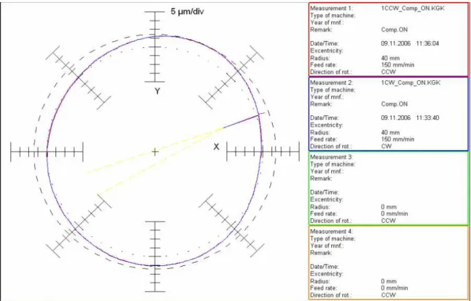
During this thesis-work there was an opportunity to make a measurement on the machine with the Heidenhain KGM [40], a measuring system that performs circle and freeform tests. It has been conducted a circular test to check how well the machine follows a commanded path. The results obtained from this test are shown in Fig. 6.1 and Fig. 6.2. It is possible to see the commanded circle (cross-hatched line) and the lines that the machine described during the moves with different parameters. There is a “calibration file” inside the axis control system that is done by the stage company and should compensate the stages errors during a movement; the calibration file gives a correction for accuracy, orthogonality, straightness and temperature errors. During the test, this calibration file was both turned on and off to see its influence on the measurement results.
Fig. 6.1- Heidenhain test results – Compensation on Fig. 6.1 shows the results obtained with the Compensation on:
• red line: feedrate of 150mm/min, radius of 40mm and Counter Clock Wise rotation (CCW);
• blue line: feedrate of 150mm/min, radius of 40mm and Clock Wise rotation (CW). No matter the direction of the movement, in Fig. 6.1 there is a constant deviation from the ideal circle of 8µm for both the lines.
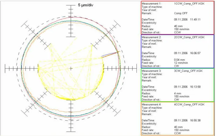
Fig. 6.2-Heidenhain test results – Compensation off
Fig. 6.2 shows the results obtained with the Compensation off in four different situations:
• blue line: feedrate of 12mm/min, radius of 0,04mm and Counter Clock Wise rotation (CCW);
• green line: feedrate of 150mm/min, radius of 4mm and Clock Wise rotation (CW);
• orange line: feedrate of 150mm/min, radius of 40mm and Counter Clock Wise rotation (CW);
• red line: feedrate of 150mm/min, radius of 40mm and Counter Clock Wise rotation (CCW). Although they have the same parameters orange and red line are different. The red line test has been done almost five hours before the other tests, so it is not comparable with the other three because of the temperature difference, in particular with the orange line one. Blue and green lines are quite similar and show a constant deviation of 5µm. Orange line is not constant and has a lot of fluctuations with a maximum deviation of 8µm.
Comparing the two figures it seems that:
• both small radius and small feedrate generate constant shape with constant deviation, while high values create a non constant behaviour with a maximum deviation;
• there is no improvement when putting the Compensation on.
The results derived from the Heidenhain KGM test, even if it has not been made many times to have a high reliability, show something that is not so fine as expected. The maximum deviation of
8µm is by far bigger than the value of the specifications, which is 2µm. This creates the need to study the dynamic accuracy of the micro-milling setup.
in order to have a better description of the dynamic performance of the machine, it has been chosen the following error – the difference between the CNC controller command position and the feedback encoder actual position reading – as a function of the acceleration. This choice is based on the concept that move durations decrease with increasing acceleration and that the short durations of high-acceleration moves create performance limitations. During each move the following error is recorded along with the servo loop commanded acceleration and the data are analysed to determine the peak following error values.
It is necessary before all else to understand the meaning of error. According to [26] the error can be understood as any deviation in the position of the cutting edge from the theoretically required value to produce a work-piece of the specified tolerance. The extent of error in a machine gives a measure of its accuracy.
The conditions for an individual test are calculated based on the desired test acceleration magnitude and the relationship between feed rate and linear acceleration to determine the velocity associated with that acceleration. Tests are run for a range of commanded acceleration values (and associated velocities) between the minimum and maximum values appropriate for the mMT being evaluated. Acceleration requirements driven by the minimum chip thickness effect manifest themselves during acceleration from a stop position and during moves such as a certain contour. In either case, acceleration requirements are established to minimize the number of tool revolutions that occur below the feed rate required by the minimum chip thickness. For acceleration from a stop, bounds can be placed on the required acceleration based on the maximum distance the machine is allowed to traverse below its required feed rate (the acceleration distance). For example, if 10µm is chosen as the acceleration distance then the required acceleration magnitude is 1,4~12,8m/s2 (0,1~1,3G) to achieve a 320~960mm/min feed rate (typical value of existing spindle technology). Bounding the allowable acceleration distance to two complete rotations of the tool (two-tool revolutions rule) creates even more severe acceleration requirements: 7~21m/s2 (0,7~2,1G) for 320~960mm/min feedrate, a 1600000rpm spindle and a 2-fluted endmill.
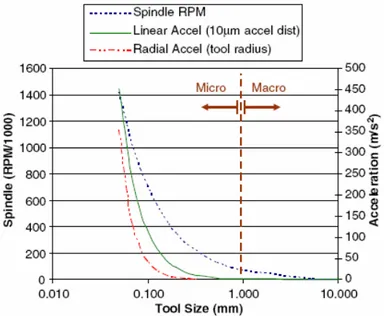
Fig. 6.3 summarises feedrate and acceleration requirements as they are driven by tool size across both macro- and micro-machining. It shows the high spindle speeds (left vertical scale) and accelerations (right vertical scale) required in micro-machining using a 224m/min surface speed and acceleration requirements based on both a 10µm acceleration distance and a radius equal to the size. As shown in the figure, spindle speeds and acceleration requirements are one to two orders of magnitude larger for tool diameters between 50 and 250µm than they are for macro-scale tools.
6.2
Design of method
The range of the acceleration test parameters for a specific mMT is determined based on the spindle speeds and feature size requirements for that machine. In the literature [20] it has been developed a comparison among three means of acceleration profiles, which can be used in machining operations: constant, linear and sine profile. Fig. 6.4 shows an example of constant acceleration test moves (two acceleration magnitudes and associated velocities).
Fig. 6.4-Example of constant acceleration and velocity test moves
Results showed that the linear and sine acceleration profile produce following errors that are about half the magnitude of the following errors measured with the constant acceleration moves. Thus, it appears that the latter profile provides the worst case of following error. Therefore in order to consider the proper worst case in this survey a constant acceleration profile is chosen.
Once upon a range of acceleration will be found, the machine will be moved with a constant acceleration profile and the following error will be estimated.
As mentioned before, in the model proposed in [20] two main methods to evaluate the acceleration requirement have been found: the first concerns about the value of the distance trajectory, while the second is based on the two-tool revolution theory, which counts on accelerating to the required feedrate in two revolutions of the tool. In both the cases the acceleration requirement depends also on the chip-load. It follows a brief explanation of the two mentioned methods:
• in the “distance trajectory method” the acceleration requirement is determined from a known distance trajectory s with a known chip-load h:
] / [ 60 mm s nhz V = (6.1) ] / [ 2 2 2 s mm s V a= (6.2)
where n is the spindle speed, z the number of cutting edge, V is the feedrate and a is the acceleration;
• in the “two-tool revolutions method” the acceleration requirement is determined from a known number of tool revolutions and a known chip-load h:
] [ 2 s n rev t = (6.3) ] / [ 60 mm s nhz V = (6.4) ] / [mm s2 t V a= (6.5)
where t is the time.
In this work it has been decided to follow the method based on the distance trajectory, thus, by setting spindle speed and number of cutting edge, the acceleration requirements correspond to certain chip-load and displacement. It is necessary at this point to fix a minimum and a maximum acceleration value.
The minimum acceleration requirement is related to the minimum chip thickness theory (see Chapter 2).
Assuming the maximum spindle speed n of the machine and the minimum chip-load hm as the 30% of the cutting edge tool radius Re, the lower acceleration requirement is determined from a move on a slot of 5mm, whose 10% is used to accelerate and decelerate (thus 5% of that to accelerate).
Starting from the following values:
rpm n=120⋅103 2 = z m Re =1
µ
m r hm =0,3 =0,3µ
mm mm s=0,05⋅5 =0,25where z is the number of cutting edge and s is the displacement, applying (6.1) and (6.2) the minimum feedrate Vmin and the lower acceleration requirement amin are obtained:
s mm z nh V m / 2 , 1 60 min = = 2 2 min 2,88 / 2s mm s V a = =
In order to evaluate the upper acceleration requirement it has been decided to use the maximum acceleration value that the machine can reach. Given that the machine can at the most reach an acceleration of 3G, it has been chosen to assume preventively a maximum acceleration requirement of 2G.
Based on the 120000rpm spindle available on the machine the acceleration requirements are determined to range between 2,88mm/s2(0.006G) and 19,6m/s2 (2G).
In order to have a more accurate analysis of the following error behaviour as a function of the acceleration, it has been thought to observe that behaviour for not only the minimum and maximum values but several intermediate values of acceleration. In the range from 2,88mm/s2 to 2G, the following values are going to be used:
2 1 2,88mm/s a = 2 2 4900mm/s a =
2 3 9800mm/s a = 2 4 14700mm/s a = 2 5 2G 19600mm/s a = =
6.3
Experimental setup
The procedure that has been applied consists of moving one stage while keeping the other stage steady (at three different positions separately, 0mm, 50mm, 95mm). This procedure is supported by the Automation 3200 (see Chapter 4), the control software of the machine from Aerotech.
The NC commands in the case of the X axis’ following error evaluation are listed below as an example.
First it is necessary to place the stage that remains steady in the fixed position (in the example Y=0mm, the “home” position) and the other one in the initial position, ready for the move (X=5mm); then it is required to set up the parameters, such as the absolute position and the units; it follows the setting of the way to move the stage (a linear velocity) giving the acceleration value; finally by the window command the X stage is moved to the final position resulting from a displacement of 0,25mm, 0,5mm or 1mm. The commands used in case of acceleration a1 are:
ENABLE Y HOME Y
G90 (Absolute programming mode, to set the absolute position) G71 (Metric unit programming mode, to set metric unit)
G76 (Distance units/second, to set distance unit/second for the velocity) RAMP MODE RATE (Specify rate-based ramping mode)
RAMP MODE LINEAR (Specify linear ramping mode, to choose a linear velocity) RAMP RATE “acceleration value” (Set ramp rate)
G1 X5 F2 (Linear interpolation (G1) and Linear feedrate specifier (F), to move linearly X in 5mm, the initial position, with a maximum velocity of 2mm/s)
GI X5.5 F2 (move X for 0.5mm)
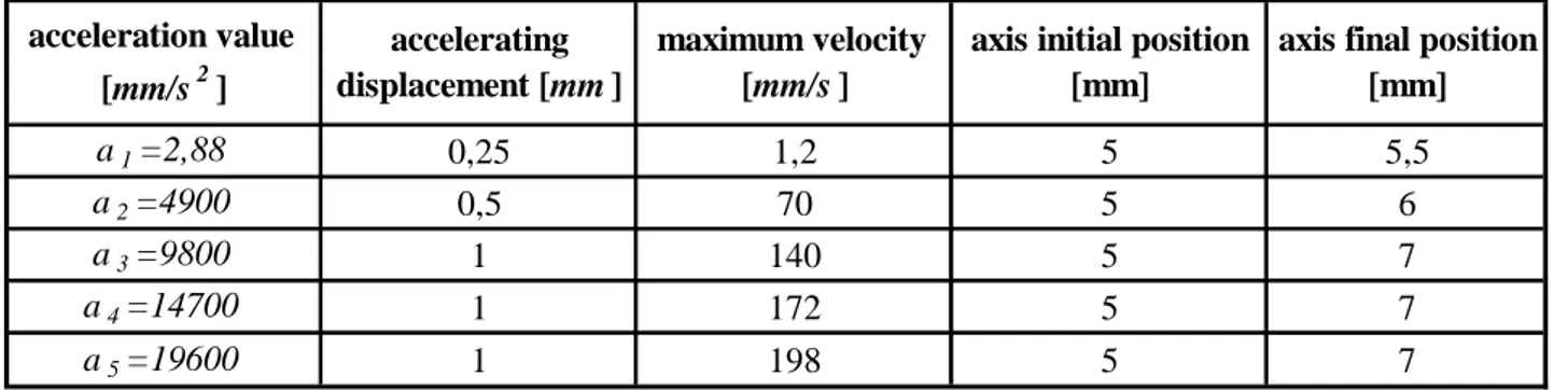
Tab. 6.1 shows the values of initial and final position, displacement and velocity related to the acceleration values.
Tab. 6.1- Values of initial and final position, displacement and velocity
6.4
Experimental results
As it is noticeable in the Tab. 6.1 the velocity value related to a1 acceleration and the displacement of 0,25mm is in accord with the relation V = 2⋅ ⋅a s, where a is the acceleration and s is the displacement. a1=2,88 0,25 1,2 5 5,5 a2=4900 0,5 70 5 6 a3=9800 1 140 5 7 a4=14700 1 172 5 7 a5=19600 1 198 5 7
axis initial position [mm]
axis final position [mm] acceleration value [mm/s2] accelerating displacement [mm ] maximum velocity [mm/s ]
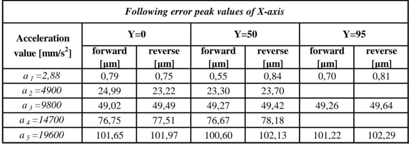
Tab. 6.2- Maximum values of the following error related to the X axis
As described before during the move the velocity increases and decreases linearly. The distance written under the column accelerating displacement in the Tab. 6.1 is the displacement during which the acceleration acts. The same slot is necessary for the deceleration, this is the reason why the distance between the initial and the final position is double of the displacement.
In order to show the worst following error of the machine it has been decided to consider the maximum values obtained during the moves of the stages, though having recorded the behaviour of the following error along the whole displacement.
Tab. 6.2 shows the maximum values of the following error related to the X axis when the steady stage’s position is Y=0mm, Y=50mm and Y=95mm. Some values in the Y=95mm column are missed because those measurements have not been done in order to speed up the experiment.
Fig. 6.5 displays only the behaviour of the X axis when Y=50mm, because it is the same in the other two positions.
Fig. 6.5- Behaviour of the X axis when Y=50mm
X following error Y=50mm y = 0,0052x - 0,4929R2 = 0,999
0 20 40 60 80 100
0,00E+00 5,00E+03 1,00E+04 1,50E+04 2,00E+04
acceleration [mm/s2] fo ll o w in g e rr o r p e a k [ u m ]
X_Y=50 forward X_Y=50 reverse Lineare (X_Y=50 forward)
a1=2,88 0,79 0,75 0,55 0,84 0,70 0,81 a2=4900 24,99 23,22 23,30 23,70 a3=9800 49,02 49,49 49,27 49,42 49,26 49,64 a4=14700 76,75 77,51 76,67 78,18 a5=19600 101,65 101,97 100,60 102,13 101,22 102,29 forward [µm] reverse [µm] forward [µm] reverse [µm] Following error peak values of X-axis
Acceleration
value [mm/s2]
Y=0 Y=50 Y=95
forward [µm]
reverse [µm]
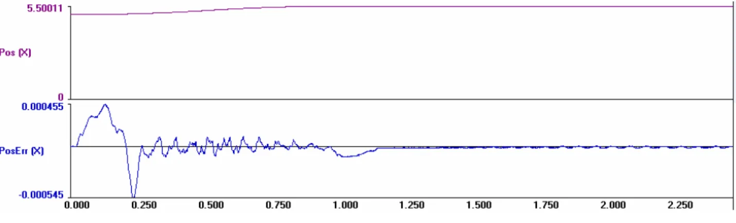
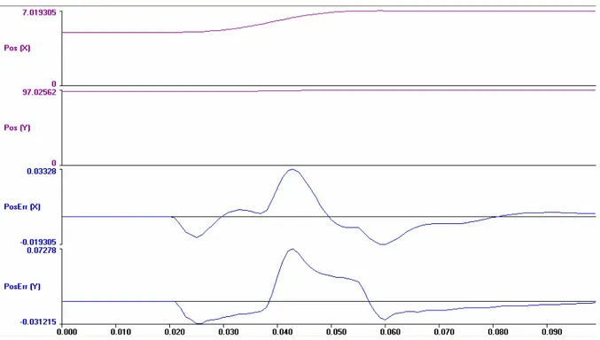
Fig. 6.6 displays the behaviour of the X axis following error in the forward case with an acceleration value of 2,88mm/s2. In the abscissa axis is the time in second and in the ordinate axis is the following error value in micron.
It is possible to see in that graph that the peak value of the following error is 0,55µm, which is also shown in Tab. 6.2 at the corresponding acceleration value. The behaviour of the following error oscillates visibly for the first second and then it is quite stable.
Fig. 6.6- X axis following error in the forward case with an acceleration value of 2.88mm/s2 In the same way Tab. 6.3 and Fig. 6.7 describe respectively peak values (when X=0mm, X=50mm and X=95mm) and behaviour (only when X=0mm) of the following error related to the Y axis. There are data missing in the X=50mm and X=95mm columns because those measurements have not been done in order to speed up the experiment.
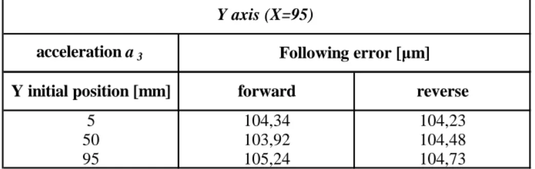
It is shown below the behaviour of the following error when, fixed the steady stage’s position, it has been changed the initial position of the moving stage. Tab. 6.4 and Tab. 6.5 show respectively the results of those proofs in three different initial positions for the steady positions Y=0mm and X=95mm withan acceleration value of 9800mm/s2.
a1=2,88 1,37 1,40 1,37 1,37 1,39 1,37 a2=4900 53,78 53,46 a3=9800 104,34 104,23 105,44 104,13 105,29 103,90 a4=14700 144,93 145,26 a5=19600 192,22 192,61 192,50 192,54 192,24 192,39 reverse [µm] forward [µm] reverse [µm] Following error peak values of Y-axis
Acceleration value [mm/s2] X=0 X=50 X=95 forward [µm] reverse [µm] forward [µm]
Fig. 6.7- Behaviour of the Y axis when X=0mm
Tab. 6.4- Results of X axis following error test (Y=0mm)
Tab. 6.5- Results of Y axis following error test (X=95mm)
So far the test includes the behaviour of the two stages moved separately. It is going to observe the behaviour of both of them when they moved together.
In this case several measurements were conducted with a combination of both stages at three different initial positions of the two stages: 5mm, 50mm, 95mm.
Y following error X=0mmy = 0,0096x + 4,7302 R2 = 0,998 0 50 100 150 200
0,00E+00 5,00E+03 1,00E+04 1,50E+04 2,00E+04
acceleration [mm/s2] m a x im u m f o ll o w in g e rr o r p e a k [u m ]
Y_X=0 forward Y_X=0 reverse Lineare (Y_X=0 forward)
5 49,02 49,49
50 47,92 49,16
95 48,59 50,60
X axis (Y=0)
acceleration a3 Following error [µm]
X initial position [mm] forward reverse
5 104,34 104,23
50 103,92 104,48
95 105,24 104,73
Y axis (X=95)
acceleration a3 Following error [µm]
Tab. 6.6- Maximum values of the following error related to the X and Y axis when Xin=5mm and Yin=5mm
Tab. 6.6, Tab. 6.7 and Tab. 6.8 show peak values of the following error related to the X and Y axes. These are just three examples of the following error obtained when the two stages were moved together, but in this survey all the combinations obtainable with the three aforementioned positions have been checked.
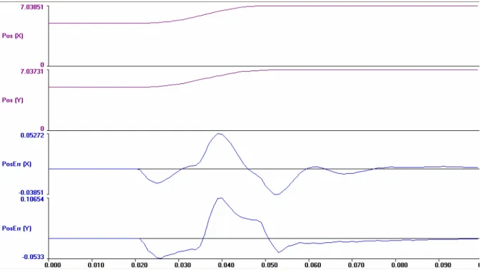
Fig. 6.8, Fig. 6.9 and Fig. 6.10 indeed display the behaviour of the two axes in three cases with an acceleration value of 14700mm/s2 (a4), 9800mm/s2 (a3) and 4900mm/s2 (a2) respectively.
Fig. 6.8- X and Y axis following error in the forward case with an acceleration value of 14700mm/s2 a1=2,88 0,57 0,74 1,12 1,27 a2=4900 14,97 14,75 36,39 36,56 a3=9800 33,11 32,86 71,96 72,16 a4=14700 52,72 52,33 106,54 106 a5=19600 60,83 59,14 113,55 112,12
Following error peak values of XY
Xin=5; Yin=5 Following error [µm]
Acceleration value
Tab. 6.7- Maximum values of the following error related to the X and Y axis when Xin=5mm and Yin=95mm
Fig. 6.9- X and Y axis following error in the forward case with an acceleration value of 9800mm/s2
Tab. 6.8- Maximum values of the following error related to the X and Y axis when Xin=50mm and Yin=95mm a1=2,88 0,46 0,74 0,50 1,02 a2=4900 14,38 15,19 35,49 37,35 a3=9800 33,35 33,70 72,68 72,08 a4=14700 52,94 53,00 106,68 105,92 a5=19600 60,18 60,79 113,03 111,7
Following error peak values of XY
Xin=95; Yin=50 Following error [µm]
Acceleration value
[mm/s2] Xforward Xreverse Yforward Yreverse
a1=2,88 0,40 0,59 0,61 1,29
a2=4900 13,94 14,60 35,35 37,79
a3=9800 31,77 31,81 72,81 73,01
a4=14700 52,81 52,60 107,29 107,35
a5=19600 59,10 58,95 113,19 113,63
Following error peak values of XY
Xin=50; Yin=95 Following error [µm]
Acceleration value
Fig. 6.11 shows the curves of the peak values of following error of X and Y stages as a function of the acceleration.
Fig. 6.10- X and Y axis following error in the forward case with an acceleration value of 4900mm/s2
Fig. 6.11- Curves of the peak values of following error of X and Y stages
XY peak following error (95;5)
R2 = 0,99 R2 = 0,9883 0 10 20 30 40 50 60 70 80 90 100 110 120 0 2000 4000 6000 8000 10000 12000 14000 16000 18000 20000 acceleration [mm/s2] p e a k f o ll o w in g e rr o r [u m ]
X-peak values_forward X-peak values_reverse
Y-peak values_forward Y-peak values_reverse
6.5
Analysis and discussion
The experiments have been conducted for each single stage in three different positions (0mm, 50mm, 95mm) but it has been noticed that the steady stage position did not influence the following error of the other stage, as demonstrated in Tab. 6.2 and Tab. 6.3.
On the contrary the initial position of the moving stage had some influence. It seems that the following error when Xin=5mm and Xin=95mm is a little bit higher than that when Xin=50mm, so as
the following error when Yin=5mm and Yin=95mm is a little bit higher than that when Yin=50mm.
As seen in the case where the two stages were moved separately, also in the case in which these were moved together, the initial position of the moving stage influenced the following error. In fact no matter what the Y initial position was, it was always observed that the following error of the X axis was bigger when Xin=5mm and Xin=95mm than when Xin=50mm. The same trend was also
observed to the following error of the Y asix when it was moved together with the X stage.
Moreover, by analysing the results of the contemporary moves of the two stages, it is noticeable a big difference between the maximum values of the Y axis following error and that of the X axis. The Y axis value in fact becomes double of the X axis value when the tested acceleration value was greater than a2 (Fig. 6.11). This phenomenon was also observed when comparing the data of only one stage moved along the other fixed; but the magnitudes in this case are bigger.
Summing up the results it has been noticed that:
• the following error of the stages is bigger at the beginning and end of travel;
• the following error is smaller when the stages were moved contemporarily than the case when only one stage was moved;
• the following error of the Y stage is bigger than that of the X stage.
These aspects can be due to the geometry of the stages and to the way of assembly. This is just a hypothesis that cannot be confirmed because it would be necessary to analyse the drawings of the stage and the way how these are mounted.
Another reason could be the fact that the Y stage is moving on the X stage, which is fixed to the basement, as if the following error of the X stage influences the one of the Y stage.
Fig. 6.8, Fig. 6.9 and Fig. 6.10 show quite the same behaviour of the following error of X and Y stage when they were moved together. The maximum error value for both the stages corresponds around to the 50% of the displacement and the range of biggest error corresponds to the central part of it where the acceleration changes sign and the velocity changes inclination, as shown in Fig. 6.4. The biggest error is around the vertex of the triangular trend of the velocity. Moreover, in the graph it can be noticed, as mentioned before, that the peak value of the Y axis is bigger than that of the X axis
In the excel graphs above it can be noticed the equation that describes the trend-line of each curve together with the R2 value, which indicates how well the trend-line reproduces the real data point. It is interesting to see in the following graph that the R2 value is almost 1, i.e. the trend-line reproduces quite exactly the curve of the peak values of the following error.
It results from the tests that the stage is not able to achieve all the peak commanded accelerations in the evaluation. This is due to the fact that actual closed-loop acceleration capability is dependent on multiple factors including moving mass, motor peak force, stage dynamics and tuning of the control loop.
It is evident from the experimental results presented above that the following error increases with the acceleration magnitude. An assessment of relative accuracy as a function of acceleration can be performed based on evaluating the following error associated with an acceleration magnitude, determining the corresponding tool size and calculating a relative accuracy between that following error and a feature size appropriate for the tool size. In the case of the 3-axis machine tested here, the results of the acceleration testing show that a relative accuracy of 10-3~10-2 can be
achieved for feature sizes around 1mm, using a 0,5mm tool and the associated motion parameters involving accelerations up to about 2,88÷4900mm/s2 (0,006÷0,5G). Under the same conditions of tool and features sizes, increasing the acceleration values the related following error increases and the relative accuracy consequentially decreases. The 3-axis machine in analysis can achieve 10-3 relative accuracy only when machining with accelerations below 9800mm/s2 (1G).
Other specific observations from these experiments are:
• micro milling operations have their own set of motion parameters, imposed by the combination of the minimum chip thickness effect and the high spindle speeds needed when using small diameter tools. These motion parameters involve minimum required feedrates of over 200mm/s, leading to acceleration requirements above 2G;
• an acceleration-based performance evaluation methodology has been used to test the setup performance which involves a series of single stage, constant acceleration, linear moves to observe the variation of following error with acceleration magnitude;
• results from testing the micro-milling machine with the new acceleration-based methodology provide a basis to determine allowable acceleration levels to achieve a relative accuracy of 10-2~10-3;
• the following error of the stages may be influenced by the controller. It would be opportune to delve into the knowledge of the control system to verify how much it influences the accuracy of the stages; in fact, as demonstrated by the Heidenhain tests, the “calibration file” of the controller seems not to make any difference of the stage behaviour by activating it or not.
• in order to improve the following error some model are proposed; in [20] for instance two models are shown: one describes the following error through the servo-frequency and the acceleration magnitude, while the other uses the servo-period and the acceleration.
In conclusion, in order to improve the micro-milling process it is better to use a low value of the acceleration magnitude so to obtain:
• a lower following error that improves the quality of the work-piece;
• a smooth movement that prevents early tool wear.
Nevertheless that disagrees with the possibility to take advantages of the potentialities of the high speed machine. It is considered opportune to do a balancing act of the two aspects respect to the single application, trying to evaluate which is the most important: either to use the high speed performance advantages or to obtain a high quality product.