Chapter 2 - Experimental set-up
The goal of this experimental work is the investigation of the hydrodynamics and the mass transfer properties of a bubble column and a packed bubble column when operated with viscous fluids.
2.1 Experimental set-up
The experimental set-up used in this work is available in the Chemical Engineering and Chemistry Department of Eindhoven University of Technology. It mainly consists of a rack with a bubble column, piping, pumps and some instrumentation.
2.1.1 Set up
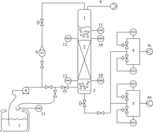
A schematic diagram of the experimental apparatus is shown in Figure 2.1.
The column used in the experiments is 29cm in inner diameter and 3m in height, it is manufactured in Perspex® (poly-methylmethacrilate), a transparent plastic that allow to check visually the bubble regime transition (Figure 2.3).
The packings rest on a support grid made in aluminium which keep the packing 22cm distant from the gas sparger. The support tray was designed basing to the Montz Support system Type G and Intalox Support grid 802, both recommended for column diameter lower than 1000mm, and manufactured in the university workshop (Figure 2.2).
Another pool of liquid is kept at a constant level on the packing to provide the complete wetting of the packing and the radial dispersion of the tracer during the axial dispersion experiment. Since it is impossible to see the flow regime in the packed column, this pool allow to see it in the moment when the bubbles come out of the packing.
The height of this pool varies from one experiment to another between 32 and 37 cm.
Figure 2.1 – Experimental set up: 1.column, 2. packing, 3. gas sparger, 4. nitrogen flow controllers, 5. air flow controllers, 6. venting, 7. liquid tank, 8. centrifugal pump, 9. liquid flow indicator,
10. oxygen sensors, 11. conductivity sensors, 12. pressure sensors
The gas sparger in the bottom of the column is a stainless steel perforated plate with 1555 holes of 0.5mm in diameter, the holes are positioned in a triangular pitch with a step of 6mm.
Figure 2.2 – Montz Support system Type G
N2 Air FIC1 FIC2 FIC3 FIC4 CIR2 PIR1 CIR1 OIR1 OIR2 PIR2 FI1 12 11 11 12 10 10 9 8 7 5 4 3 2 1 6
The column is operated in counter current with the gas flowing upward and the liquid downward.
Figure 2.3 – Column, Brooks MT 5853, DPV 4-40
2.1.2 Instrumentation
The air flow is supplied from the main tank with apposite pipeline and it is controlled by two automatic flow meter Brooks MT 5853 (Figure 2.3): the first works in the higher range 090m3/h, the second in the lower range 010m3/h, both ranges are referred to
standard condition (25°C, 1atm). The nitrogen is supplied by four parallel cylinders of a capacity of 50L eachone at the nominal pressure of 200bar and the flow rate is controlled by other two automatic flow meters Brooks MT 5853: the first works in the higher range 045m3/h, the second in the lower range 05m3/h, also these ranges are
referred to standard condition1. Before the flow controllers, the pressure is kept constant
at 5 bar by a pressure reducer, after the passage in the column, the gas is vented to atmosphere.
The liquid flows in closed loop and it is circulated by a Duijvelaar centrifugal pump DPV 4-40 (Figure 2.3). The flow rate is measured by two flow meter Brooks MT 3809 (Figure 2.10 page 32): the first operates in the range of 01000L/h and the second in the range of 01500L/h. The flow rate is adjusted manually with bulb valves both in the inlet and in the outlet line.
Both the indicators are variable area flowmeters, flow rate indication is provided by means of magnetic coupling where a magnet, encapsulated in the float, is coupled to a rotatable magnet located in the rear of the indicator, thus turning the dial indicator mounted on the meter. The indicators are equipped with a viscosity immunity ceiling which provides reliable measurements up to 250 mPa·s and 400 mPa·s respectively2.
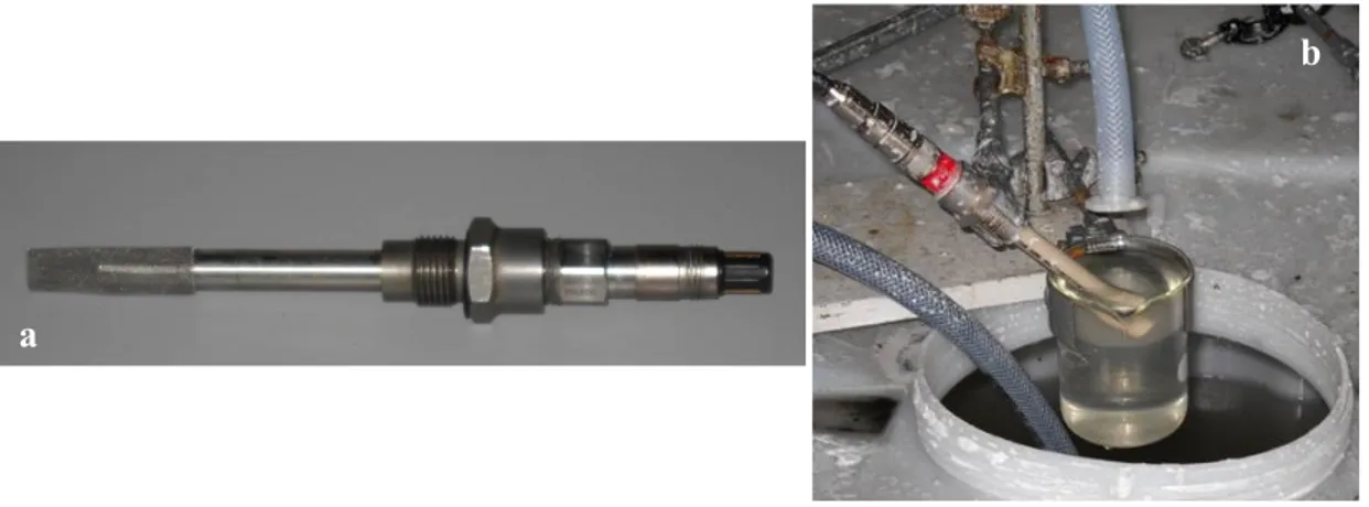
The installed sensors log temperature, pressure, conductivity and oxygen concentration of the liquid to a PC. The pressure sensors are two Endress+Hauser Cerabar T PMC131; the conductivity sensors are two Mettler Toledo InPro 7100 and the oxygen sensors are two Mettler Toledo InPro 6800 (Figure 2.4).
Figure 2.4 – a) Oxygen sensors, b) conductivity sensor
1 Brooks Instrument Product data 5850s-5864s, 2001
2 Brooks Instrument Data sheet MT3809-3819, September 2008
a
The oxygen and conductivity probes contain temperature sensors to compensate the measurements, the measuring range for the oxygen sensors is 0.26 bar and 080°C3,
for the conductivity sensors is 020bar and -20150°C4.
The sensors in the bottom of the column are installed in the same position for all of the three internals, the pressure sensor is at 14cm in height from the bottom and the oxygen sensor at 12cm. This mean that in the packed bubble column they are respectively 7 and 9cm below the packing. Since the conductivity sensor is very sensitive to the presence of gas bubble, it was positioned outside the column in a 250ml beaker at the end of the outlet line (Figure 2.4b).
In the bubble column the pressure sensor on the top is installed at 171cm in height from the gas distributor, the oxygen sensor at 181cm and the conductivity sensor at 191cm; in the SuperPak packed column the first is at 161cm, the second at 181cm and the third at 171cm, this mean that they are respectively 3, 13 and 23cm above the packing; in the Flexipac packed column the pressure sensor is at 171cm from the bottom, the oxygen sensor is at 191cm and the conductivity sensor at 181cm, this mean that they are respectively 6, 16 and 26cm above the packing.
Since the conductivity sensor is sensitive to the presence of gas bubble, it is shielded from the rest of the liquid with small piece plastic tube opened on the top (Figure 2.5).
Figure 2.5 – Sensors on the top of the column
3 METTLER TOLEDO Technical data InPro 6950/ 6900/ 6800/6050, 03/07 4 METTLER TOLEDO Technical data InPro 7100/12mm, 11/2008
All the sensors are immersed in the liquid for 12cm.
All of the sensors are connected to a computer through transmitters and dedicated signal conditioners. The data are logged continuously by a LabView software which also allow the control of the process variables and the instrumentation.
The control panel of the software is shown in Figure 2.6.
The pilot plant used in these experiments is equipped with two different column, the first is called Column B in the control panel and it is 12cm in inner diameter, the second is called Column C and it is the column used for the experiments.
The pipeline on the right side of the panel was used to feed the column in a co-current downflow regime but now it no longer exists.
2.2 Packings
The manufacturers of packings provide a very wide selection of packings optimized for very different process and operating conditions.
The main distinction among the several existing packings is between random and structured packings.
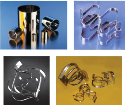
The first type consists of a large amount of small units usually randomly dumped in an empty column to enhance the mass transfer between a liquid and a gas phase. The shape of these units can differ very much from simple cylinder (Raschig Rings) to very detailed geometry with several expansions and stripes (for example Nutter Rings or Intalox Ultra). Also the size can be very wide ranged, usually from 8 to 100mm (Figure 2.7).
Figure 2.7 – Random packings: Raschig Rings, Super Rings, Intalox Ultra, IMTP
The structured packings consist of large units neatly arranged in a well defined geometry studied to enhance particular characteristic of the packing. The packing is usually manufactured in several layers to be stacked inside the column in a specific order. The most common structured packings are different variations of the corrugated sheet geometry but advanced shapes, wire gauze and grids are also used as column internal (Figure 2.8).
Figure 2.8 – Structured packing : Montz-Pak type M, Sulzer gauze type CY, Glitsch KFBE
All of the packing can be manufactured in metal or plastic, some of them also in ceramic.
The aim of this work is the characterization of the column internals for the production of polyester in a reactive packed bubble column. The molten polyester is a pretty viscous liquid and its viscosity increase as the molecular weight increase: this means that the residence time distribution curve of the liquid has to be pretty sharp in order to avoid that polymer reacts for a too long time becoming too viscous and plugging the column and to grant guarantee constant properties of the product.
Random packings have a large amount of dead volumes where capillarity forces can withhold the liquid, for this reason random packings are not considered in this work. The same remark can be applied to the gauze packing so they are also excluded.
Corrugated sheet structured packing and grids should not show this kind of issue and also have advantage of an high capacity, also required for our process because the flooding conditions can be achieved at lower gas velocity when the liquid gets more viscous.
In the reactive distillation process one of the reactant is in the gas phase and the other in the liquid phase so mass transfer efficiency is also important.
Grids have a very wide and empty structure so that residence time distribution and capacity are not a real issue but the mass transfer is quite low so they are also left out of this work.
For all of these reasons we decided that corrugated sheet and advanced geometry packing are the only one that can be suitable for this process and so we decided to test Flexipac manufactured by Koch-Glitsch and Super-Pak by Raschig Jaeger.
Flexipac –S is the simplest kind of structured packing, a corrugated sheet with a completely smooth surface. In our idea the absence of any kind of surface treatment should considerably reduce the static hold up and restrict the residence time distribution. Once listened also the manufacturer advices, we decided to test the 2X version which means a packing with a very wide open structure and an corrugation angle of 60° with respect to the horizontal (Figure 2.9a). The surface area is quite small and also the mass transfer efficiency is limited but this choice is necessary because of the viscous liquid that can increase the risk of flooding.
Super-Pak is a new generation packing, it is made of many stripes of metal stacked in several layers. The structure of this packing is very open to ensure a high capacity. The stripes usually present a textured surface but can also be manufactured smooth and for the same reason explained above this was our choice (Figure 2.9b). This structure has a high surface area and excellent mass transfer properties (in the trickling regime also because of the formation of droplet due to gas shear) but it can withhold quite high amount of liquid. The manufacturer suggested the 250Y version.
Figure 2.9 – Packings: a) Koch-Glitsch Flexipac S, b) Raschig SuperPak
In Table 2.1 are reported the most important characteristics of these packings as published by the manufacturers.
Packing Surface Area (m2/m3) Free volume (%) HETP (m) flooding (PaF-factor at 0.5)
Flexipac 2X S5 150 99 0.60-0.65 3.5
Superpak 250Y6 250 98 0.30-0.35 3.5
Table 2.1 – Packing nominal characteristics (trickling flow)
5 Koch-Glitsch Structured Packing, distillation in a “low-alfa system” at atmospheric pressure.
6 Rashig Jaeger Tecnologies Raschig Super-Pak Product Bulletin 501, C6-C7 distillation at 0.333bar
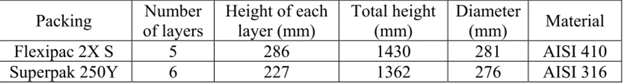
The dimensions of the packed beds are slightly different from each other because of the manufacturer’s standards and are listed in Table 2.2.
Packing of layers Number Height of each layer (mm) Total height (mm) Diameter (mm) Material
Flexipac 2X S 5 286 1430 281 AISI 410
Superpak 250Y 6 227 1362 276 AISI 316
Table 2.2 – Dimensions of the packings
2.3 Fluids
2.3.1 Liquid stream
In order to simulate correctly the hydrodynamic of the real reactive column, we need to operate the column with viscous liquids.
Kastanek, Zelenka and Hajek in 1983 developed an empirical correlation to predict the viscosity of liquid unsaturated polyester:
log · /
where:
is the dynamic viscosity in mPa·s; is the average molecular weight; is a constant and its value is 0.05; and is given by:
∞ 1 2.303 · · where: ∞ is -2.45; is 7.0·10-4 K-1; is 233.2 K.
In the case study of polyester production from maleic anhydride and propylene glycol, the average molecular number is 14, which means a molecular weight of about 2500, and the temperature is up to 300°C, extrapolating the data from their correlation we find a viscosity of about 80 mPa·s so we decided to test liquid with a viscosity up to 100 mPa·s.
An extensive research in the scientific literature showed that the viscous liquids used in this kind of experiment are water solutions of glycerol, natural polymers (i.e. starch, cellulose, agar agar, etc...) or a water soluble polymer.
According to Dow chemical data7, the viscosity of glycerol solution is pretty low and quickly increase at very high concentration. In order to achieve a viscosity of 100mPa·s at room temperature we should use a solution containing 90% of glycerol and 10% of water.
This kind of solution can lead up to some practical problem with the reliability of the data obtained in the experiments. During the experiment the gas flows through the liquid and consequently some water evaporates, because of this the liquid viscosity can change during the experiment and increase without any kind of control, so this kind of solution is not suitable for our experiment.
The natural polymers do not have this kind of issue because, according to literature, very small amounts of cellulose or agar agar can increase a lot the viscosity of water (or even transform the liquid into a gel) but they were not considered because the experiments were going to take some months and so there were the risk of growth of bacterial colonies or fungi.
For all of these reasons we decided to use a water soluble polymer and among them we opted for poly(ethylene glycol) solutions. We choose this polymer because of the large amount of data available in literature and the high solubility in water.
Poly(ethylene glycol) (PEG) is available in several molecular weight and different grade of purificaty.
In the literature several different molecular weight are used to increase the viscosity of water but only for low/medium viscosity solutions (0-20mPa·s), above this limit
mixture of different grade or mixture with agar agar are used. Anyhow usually the proposed mixtures contain about 50% by weight of PEG which is nearly equivalent to the solubility limit.
In order to enhance the reproducibility of the experiment we decided to use one only molecular weught and for the same reason explained for glycerol we decided that the maximum concentration of PEG should not be too close to the saturation.
Low molecular weight (MW≤600) are liquid at room temperature, they could be easy to handle and to dose when preparing the mixture but, according to the VWR catalogue specifications but their solutions are not viscous enough for our purpose. The same thing applies to the fractions with a molecular mass lower than or equal to 4000 where the 50% solution has viscosity up to 115 mPa·s.
Therefore we decided to test the poly(ethylene glycol) with a molecular weight of 10000.
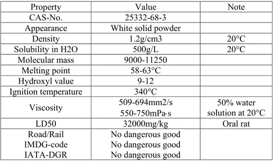
At the end of the experiment we decided that poly(ethylene glycol) with an average molecular mass of 10000 is suitable for our purposes. It was purchased from VWR and were industrial grade, the main properties are reported in Table 2.3.
Property Value Note CAS-No. 25332-68-3
Appearance White solid powder
Density 1.2g/cm3 20°C Solubility in H2O 500g/L 20°C Molecular mass 9000-11250 Melting point 58-63°C Hydroxyl value 9-12 Ignition temperature 340°C
Viscosity 509-694mm2/s 550-750mPas solution at 20°C 50% water
LD50 32000mg/kg Oral rat Road/Rail IMDG-code IATA-DGR No dangerous good No dangerous good No dangerous good
Table 2.3 – Poly(ethylene glycol) properties
The solutions were prepared at different concentration to test the column behaviour with different liquid viscosity up to 100 mPas. According to the literature, the effect of
viscosity on the column hydrodynamic and the mass transfer is pretty high in low viscosity liquids but it has less importance when the viscosity gets higher. For this reason we decided to test the following liquids: the physical properties are summarized in Table 2.4 (cf. Chapter 3).
Viscosity (mPas) Concentration (% weight) Density (kg/m3)
1 0 1000 5 8.29 1012 10 13.32 1022 25 20.68 1035 50 26.68 1046 100 32.59 1058
Table 2.4 – Physical properties of the viscous solutions at 22°C
2.3.2 Gas stream
In order to evaluate the mass transfer the gas stream is switched between air and nitrogen, both of them are supplied by Linde.
2.4 Experimental design
We already discussed about the viscosity of the liquid we decided to test. About the liquid and gas velocities we performed some preliminary tests to evaluate the maximum capacity of the column.
The tests showed that the maximum gas flow rate is 90m3/h and the maximum liquid flow rate is 720L/h (cf. Chapter 3.2). These flow rate correspond to superficial velocities of respectively 37.8cm/s and 0.303cm/s.
We decided to operate the column with five different gas and liquid flow rates.
In order to use the same conditions in all of the experiment, we decided to perform all the tests in the same range 0÷720L/h. Since these tests were performed with water in the bubble column and both the presence of the packing and the higher liquid viscosity can reduce this capacity, we decided to carry out the experiment in a smaller range 0÷500L/h, therefore the maximum liquid velocity is 0.21cm/s.
The liquid flow rate has to be adjusted manually watching at the flow indicator mounted in the piping: it shows the flow rate with a pointer moving on a scale with notches every 20L/h (Figure 2.10) so we decided to use the flow rate in Table 2.5 in the first column.
Figure 2.10 - Brooks MT 3809
The gas flow rate it is automatically controlled by the PC. Numerically, it has an accuracy of several digit after the decimal point but to be sure that the results are reliable we decided to use only an integer number of cubic meters per hour.
The data available in literature cover a wide range of gas velocities, anyhow the bubble regime transition is between 10 and 30 cm/s depending on the packing installed in the bubble column and the liquid velocity, so we decided to use superficial gas velocities up to 10cm/s (Table 2.5). Flow rate (L/h) Superficial velocity (cm/s) Flow rate (m3/h) Superficial velocity (cm/s) 0 0 5 2.103 120 0.05 10 4.205 240 0.101 15 6.308 360 0.151 20 8.411 480 0.202 25 10.514 Liquid Gas
Since we have to repeat the experiment three times, one for the bubble column and three for the two different packings, the full set of experiment involves 450 experiment so that an accurate experimental design is necessary to reduce the number of tests.
The Engineering Statistic Handbook of NIST suggests several different ways to choose the proper experimental design depending on the final objective of the experimental activity and the number of variables.
The most important criteria are summarized in Table 2.6. Number of
variables
Objective
Comparative Screening Response surface
1 1-factor completely randomized design - -
2-4 Randomized block design Full or fractional factorial Central composite or Box-Behnken 5 or more Randomized block design
Fractional factorial or Plackett-Burman
Screen first to reduce the number
of factors
Table 2.6 – Experimental design selection guideline
In this work we want to evaluate the dependence of some properties with the gas velocity, the liquid velocity and the liquid viscosity; so the choice is between the central composite and the Box-Behnken design.
The Box-Wilson Central Composite Design, commonly called `a central composite design,' contains a full factorial or fractional factorial design with centre points that is enhanced with a group of `star points' that allow estimation of curvature (Figure 2.11).
Figure 2.11 – Generation of a central composite design for two factors
A central composite design always contains twice as many star points as there are factors in the design and they represent the extreme values (low and high) for each factor
in the design. Three different varieties of central composite designs are commonly used: circumscribed, inscribed and face centred designs.
Circumscribed central composite designs (CCC) are the original form of the central composite design. The star points establish new extremes for the low and high settings for all factors. These designs have circular, spherical, or hyperspherical symmetry and require 5 levels for each factor. Augmenting an existing factorial or resolution V fractional factorial design with star points can produce this design.
Inscribed central composite designs (CCI) uses the factor settings as the star points and creates a factorial or fractional factorial design within those limits for those situations in which the limits specified for factor settings are truly limits (in other words, a CCI design is a scaled down CCC design with each factor level of the CCC design divided by to generate the CCI design). This design also requires 5 levels of each factor.
In the face centered central composite designs (CCF) the star points are at the center of each face of the factorial space. This variety requires 3 levels of each factor. Augmenting an existing factorial or resolution V design with appropriate star points can also produce this design.
Figure 2.12 illustrates the relationships among these varieties.
Figure 2.12 – Pictorial representation of the three type of CCD
Note that the CCC explores the largest process space and the CCI explores the smallest process space. Both the CCC and CCI are rotatable designs, but the CCF is not.
The Box-Behnken design is an independent quadratic design in that it does not contain an embedded factorial or fractional factorial design. In this design the treatment combinations are at the midpoints of edges of the process space and at the center. These designs are rotatable (or near rotatable) and require 3 levels of each factor. The geometry of this design suggests a sphere within the process space such that the surface of the
sphere protrudes through each face with the surface of the sphere tangential to the midpoint of each edge of the space (Figure 2.13).
Figure 2.13 - A Box-Behnken Design for Three Factors
Since we already planned five levels in the gas and liquid velocity and six in the viscosity and the Box-Behnken design does not provide sufficient accuracy, in this work the central composite design have been chosen (yellow flags in Figure 2.14).
This model requires and takes into account five levels in each variable, it means that it fit with the decided step in the gas and liquid velocity but not with the six step planned for the liquid viscosity. In order to overcome this discrepancy we decided to apply the central composite design only to the five higher level of the viscosity and add to add few other experiment to describe the lowest level. The reasons of this choice rely on the fact that a large amount of data, available in literature, can be used to describe this condition (liquid viscosity similar to water) and on the idea that only a small part of the column we want to model works with this liquid viscosity. The experiment planned in this level (green flags in Figure 2.14) were chosen in order to replicate the conditions of the higher levels to evaluate the curvature of the response surface.
In order to analyze better the behaviour of our system with the process variable, we decided to add few experiments to have the full data set in particular conditions (listed Table 2.7 and reported as red flags in Figure 2.14).
Gas flow rate Liquid flow rate Viscosity
Any 240L/h 25 mPas
15m3/h Any 25 mPas
15m3/h 240L/h Any
The experimental data in these conditions will be used to evaluate the behaviour of the interested properties with the process variable and develop the proper correlation, then the data collected in the other experiments will be used to tune the numerical constants in order shift the same curve to a different level and adjust the curvature.
Few other point are added to better define the condition neglected in the central composite design (blue flags in Figure 2.14).
Consequently to this experimental design, the number of experiment decrease from 450 to 126. 0 120 240 360 480 0 120 240 360 480 0 120 240 360 480 0 120 240 360 480 0 120 240 360 480 5 10 15 20 25 5 10 15 20 25 5 10 15 20 25 5 10 15 20 25 5 10 15 20 25 5 10 15 20 25 Central composite design 15 Full resolution 7 Improving resolution 16 Lowest viscosity 4 Total 42x3=126
Liquid flow rate (L/h) Liquid flow rate (L/h)
G as fl ow r ate (m 3 /h)
Liquid flow rate (L/h) Liquid flow rate (L/h) Liquid flow rate (L/h)
vi sc os ity cP 1 5 10 25 50 100
Figure 2.14 – Experimental design
2.5 Procedures
At the beginning of the experiment the column is filled of liquid from the bottom, the liquid is not fed from the top because the jet would hit the sensors on the top damaging them. A minimum air flow of 1m3/h is used to prevent the liquid from passing through the gas distributor and clogging the gas pipe.
When the column is almost full, the air flow rate is set to the right value and the column is filled to the top, the inlet flow is set referring to the flow meter while the outlet is adjusted checking the liquid level in the column.
The first experiment performed is about the axial dispersion: 500mL of saturated solution of sodium chloride is poured on the top of the column, then we have to wait until the conductivity measurements on the top and the bottom of the column are stable.
Then the mass transfer experiment starts: the gas flow switches from air to nitrogen and the oxygen readings start decreasing, when both of them are below 1mg/L this experiment is also finished.
The pressure difference necessary to evaluate the gas hold up is continuously during the previous experiments.
At the end of the experiments, the gas flow goes back to 1m3/h of air and the column is drained.
Referring to Figure 2.15 (below), the procedure for the experiment is as follows: 1. Power up the plant and the control system;
2. Start the LabView software;
3. Open the automatic valves FS4 and FS7;
4. Open the manual valves FS15, FS16, FS18, FS23; 5. Start a minimum air flow (1m3/h);
6. Start the pump M3 and fill the column with liquid;
7. When the column is half-full, set the air flow to the desired value; 8. Open the automatic valve FS1;
9. Close the automatic valve FS4 and manual valve FS16;
10. When the column is full, manually set the liquid flow in the inlet piping using valve FS18 and the flow indicator;
11. Manually adjust the outlet liquid flow using valve FS14 and checking the level in the column;
Start of the experiment
12. Pour 500mL of saturated solution of NaCl on the top of the column;
13. Check the values of the conductivity measurements and wait until the values are stable for 2 minutes;
14. Open the nitrogen cylinders;
15. Switch the gas flow from air to nitrogen;
16. Check the values of the oxygen measurements and wait until both values fall below 1mg/L;
End of the experiment
17. Switch the gas flow back to air and the rate to 1m3/h; 18. Close the nitrogen cylinder;
19. Switch off the pump M3;
20. Drain the column opening valve FS14 completely; 21. Close the automatic valves FS1 and FS7;
22. Shut down the LabView software; 23. Shut down the plant instrumentation.