Dipole and rotational strengths for overtone transitions of a C2-symmetry HCCH molecular fragment using Van Vleck perturbation theory

Dipole and rotational strengths for overtone transitions of a

C

₂

-symmetry

HCCH molecular fragment using Van Vleck perturbation theory

Sergio Abbate, Roberto Gangemi, and Giovanna Longhi

Dipartimento di Scienze Biomediche e Biotecnologie, Universita` di Brescia, via Valsabbina 19, 25123 Brescia, Italy and INFM, Udr Brescia, via Valotti 9, 25133 Brescia, Italy

共Received 23 May 2002; accepted 15 July 2002兲

Contact transformation theory up to second order is employed to treat CH-stretching overtone transitions and to calculate dipole and rotational strengths. A general Hamiltonian describing two interacting CH-stretching oscillators is considered, and the Darling–Dennison resonance is appropriately taken into account. The two CH bonds are supposed to be dissymmetrically disposed, so as to represent a chiral HCCH fragment, endowed withC2 symmetry. Analytical expressions of

transition moments and dipole and rotational strengths are given in the hypothesis of general electric and magnetic dipole moments with quadratic dependence on coordinates and momenta. Dipole and rotational strengths are then calculated together with frequencies for the fundamental and first three overtone regions in the simplifying hypothesis of the valence optical approach on the coupled-oscillator framework. Simplified analytical expressions thereof in the relevant parameters are presented. © 2002 American Institute of Physics. 关DOI: 10.1063/1.1504705兴

I. INTRODUCTION

A renewed interest in measuring vibrational circular di-chroism 共VCD兲 spectra in the CH stretching overtone region1–3 has raised the necessity of calculating overtones’ rotational strengths.4For this reason we have undertaken the study of a simplified model consisting of two coupled oscil-lators described by a two-degrees-of-freedom Hamiltonian including Darling–Dennison 共DD兲 terms.5 This kind of dy-namical model has been demonstrated to be quite appropriate to study both fundamental and overtone transitions, and has been extensively studied in the literature by means of second-order perturbation theory,6by integration of classical equations of motion, and semiclassical quantization of trajectories.4,7–9We adopt here the method of Van Vleck con-tact transformations, for the main reason that these transfor-mations can be easily applied to operators, permitting one to examine the analytical expressions of the electric and mag-netic dipole moments treated at any desired order.

The contact transformation formalism was originally de-veloped for accurately calculating frequencies and for inter-preting high-resolution spectra of molecules in the gas phase.10–13Afterwards, it was also adapted and used for cal-culating dipole and rotational strengths in the infrared range.14 –16 Expressions for dipole and rotational strengths for overtone transitions have been obtained by Bak et al.17 and Polavarapu18 for a single chiral oscillator and by ourselves4for a system of two oscillators with strong simpli-fying assumptions that will be abandoned in this paper. More recently, the same perturbative method has been applied to study vibrational manifolds, which are important for over-tone spectroscopy, with quite high orders of perturbative terms and increasing number of degrees of freedom.19

We have limited ourselves here to a simple two-oscillator model and to low perturbative orders to handle simple analytical results. We have studied the system of two

interacting CH stretches in a dissymmetric HCCH molecular fragment共Fig. 1兲, with the additional requirement that it pos-sess aC2-symmetry axis bisecting the CC bond; this requisite

does not prevent it from exhibiting optical activity. Our choice is motivated by the fact that it is the simplest coupled-oscillator model and is still extensively applied for the inter-pretation of spectra of CH stretching vibrations in many chi-ral molecules.20–23 The model is adequate when the CH stretchings can be regarded as dynamically and possibly electrically 共as we will discuss later兲 isolated from other vi-brational modes. If the valence angles and the dihedral angle in this fragment are fixed, two normal modes are present, one being symmetric and the other antisymmetric with respect to the C2-symmetry axis: let the corresponding normal-mode

dimensionless coordinates and conjugated momenta be de-noted by qs, ps and qa, pa, respectively. Let the

corre-sponding frequencies in wave number units be ␻s and␻a,

respectively. Following the notation of Ref. 4, the general Hamiltonian possessingC₂ symmetry at fourth order is

H⫽H0⫹␧H1⫹␧2H2, 共1兲 where H0⫽共hc/2兲兵␻s关共ps/ប兲2⫹qs 2_兴⫹␻ a关共pa/ប兲2⫹qa 2_兴其, 共1⬘兲 ␧H1⫽hc关Ksssqs 3_⫹K saaqsqa 2_{兴, 共1⬙兲} ␧2_H 2⫽hc关Kssssqs 4_⫹K aaaaqa 4_⫹K ssaaqs 2 q_a2兴. 共1⵮兲

In Ref. 4 drastic assumptions regarding anharmonic force constants were made; i.e., only diagonal cubic and quartic terms Kiii and Kiiii were assumed to be different from zero

共the index i denotes a generic normal mode兲; this simplifica-tion allows one to avoid the problem of resonances and as-similates the many-oscillator problem to the one of a single oscillator. We stated, however, that the inclusion of the inter-7575

action term Kii j j(i⫽ j) is necessary, as had been pointed out

by many authors,24 –27in order to account for the transition from the normal-mode regime to the local-mode regime.28 The inclusion of the Kii j jterm is essential to demonstrate the

equivalence of a normal-mode Hamiltonian with anharmonic interactions, like the one we use here, to the Hamiltonian of harmonically coupled anharmonic oscillators 共for a review, see Ref. 6兲.

Hamiltonian 共1兲 coincides with the one that Mills and Robiette used for water in normal coordinates.26The equiva-lence between the normal-mode scheme and the local-mode scheme, proved by way of a variational perturbative treat-ment, implies the existence of appropriate relations between the parameters ␻0, ␹ of the bond Morse potential in local

coordinates and the anharmonic coefficients Ki jk, Ki jkl

关these relations are reported for completeness in Appendix A, Eq. 共4兲兴. Appendix A comprises the general expressions of the frequencies␻sand␻a and of the anharmonic cubic and

quartic force constants for two interacting Morse oscillators. In the present work, the contact transformation approach has to be carried out at least to second order共two contact trans-formations兲 and in resonance form, since the resonance ap-pears at second order. In fact, we shall show that these con-tact transformations at second order give the same matrix elements for the Hamiltonian and, accordingly, the same en-ergy levels as obtained in the perturbative treatment by Mills and Robiette.26

II. DETERMINATION OF CONTACT TRANSFORMATIONS

Let us briefly recall the contact transformation procedure to illustrate the notation that we are going to use and to introduce all the elements needed to obtain the transformed operators.

The first contact transformation is generated by an op-erator T1⫽exp(i␧S1)⫽1⫹i␧S1⫹¯ that acts on a generic

op-erator fˆ analogously to the Lie transformations29–31in clas-sical mechanics; formally, one can express the transformed operator fˆ

⬘

as fˆ

⬘

⫽T1• fˆ•T1⫺1⫽

兺

S 共i␧兲S s! 关S1, fˆ兴 S_{, 共2兲} with关S₁, fˆ兴S_⫽关S

1,关S1,...,关S1, fˆ兴兴兴; that is to say, the

com-mutation 关S1,...兴 is applied s times on fˆ. When this

trans-formation is applied to H, it gives

H

⬘

⫽T1•H•T1⫺1⫽H0

⬘

⫹␧H1

⬘

⫹␧ 2_H

2

⬘

⫹¯ . 共3兲

The requirement that one imposes in order to determine the generating function S1 is that the off-diagonal elements of

␧H1

⬘

, evaluated on the product harmonic oscillator

eigen-function basis, vanish at first order. We denote by 兩ns,na

典

n

the normal-mode basis 共uncoupled harmonic oscillators兲. This is exactly equivalent to saying that the eigenfunctions of the complete Hamitonian H are obtained at first order in␧ by

T₁⫺1兩n_s,n_a

典

_n. Since H₁ contains odd powers of the coordi-nates, the requirement _n

具

n_s

⬘

,n_a

⬘

兩H₁

⬘

兩n_s,n_a

典

_n⫽0, if n_s

⬘

,n_a

⬘

⫽ns,na, corresponds to imposing that i关S1,H0兴⫽⫺H1and

to reducing Eq. 共2兲 to the following conditions:

H₀

⬘

⫽H0, 共4兲

H₀

⬘

⫽0, 共4⬘兲

H₂

⬘

⫽H2⫹ i

2关S1,H1兴. 共4⬙兲

The transformation S1 obtained in this way contains new

terms with respect to those of Ref. 4, due to the presence of cubic ‘‘nondiagonal’’ perturbative terms, and S1 turns out to

be10 S1⫽Ssssps 3 ⫹共1/2兲Sss s_共p sqs 2_⫹q s 2 ps兲⫹Ssaapspa 2 ⫹共1/2兲Ssa a _q s共paqa⫹qapa兲⫹Saa s _p sqa 2_{. 共5兲}

The five coefficients depend on the cubic force constants

Ksssand Ksaa as reported in Appendix A.

With the aim of treating contact transformations at suc-cessive orders and of calculating transition moments for elec-tric and magnetic dipole moments, we used the algebraic manipulator MAPLE.32 This package gives one the opportu-nity to work with noncommutative algebras and has allowed us to easily evaluate complicated matrix elements of harmonic-oscillator eigenfunctions.

As indicated before, it is essential to consider at least a second contact transformation, thus diagonalizing the Hamil-tonian at second order. There are many reasons to go to second order. The first reason is that the anharmonic behav-ior of bond-type oscillators is well described by cubic and quartic force constants; stopping at first order permits one to deal with just cubic force constants and does not allow one to obtain energy levels in correspondence with those spectro-scopically observed for the isolated oscillator and to give a description equivalent to the well-accepted models present in the literature.33 Second, in the case of more than one oscil-lator, the importance of the DD 共Refs. 5, 25, and 26兲 inter-action terms has been recognized to cause a 2:2 resonance and thus one must go to second order. Last but not least, mechanical and electrical anharmonicities beyond first order are essential for an acceptable description of overtone ab-sorption intensities.34 –36

The implementation of procedures based onMAPLEleads first to determine the transformation T2⫽exp(i␧2S2)⫽1

⫹i␧2_S

2⫹¯ that diagonalizes the Hamiltonian terms at next

order. In analogy to Eq. 共2兲 one obtains, for a generic fˆ

⬘

, FIG. 1. Definition of the HICICIIHIIdissymmetric system and of dihedral

angle␸between planes HICICIIand HIICIICI: front view共Newman

fˆ⫹⫽T2• fˆ

⬘

•T2⫺1⫽

兺

S 共i␧2_兲S s! 关S2, fˆ

⬘

兴 S_{. 共6兲} Being H⫹⫽H₀⫹⫹␧•H₁⫹⫹␧2_•H 2 ⫹_{, we obtain} H₀⫹⫽H₀

⬘

, 共7兲 H₁⫹⫽H₁

⬘

, 共7⬘兲 H₂⫹⫽H₂

⬘

⫹i关S₂,H₀兴. 共7⬙兲 As well described in Ref. 11, S₂ must be determined by the requirement that off-diagonal terms be eliminated from

H2⫹. Beside that, one has to choose an S2 of the form given

in Eq.共8兲 below to guarantee that H₂⫹-diagonal terms remain unchanged: S2⫽Ss sss_{共1/2兲共q} sps 3_⫹p s 3_q s兲⫹Ssss s _{共1/2兲共p} sqs 3_⫹q s 3_p s兲 ⫹Sa aaa 共1/2兲共qapa 3_⫹p a 3 qa兲⫹Saaa a 共1/2兲共paqa 3 ⫹qa 3 pa兲⫹Ss aas 共1/2兲pa 2 共psqs⫹qsps兲 ⫹Sa ass_共1/2兲p s 2_共p aqa⫹qapa兲⫹Saas s _共1/2兲q a 2_共p sqs ⫹qsps兲⫹Sass a _共1/2兲q s 2_共p aqa⫹qapa兲. 共8兲

The eight coefficients S_ssss– S_assa can be determined by the condition n

具

ns,na兩H2⫹兩ns

⬘

,na

⬘典

n⫽0, if ns

⬘

,na

⬘

⫽ns,na, in

the nonresonant case. This condition can be written explicitly in the following way:

n

具

ns,na兩H

⬘

2兩ns

⬘

,na

⬘典

n⫽⫺in

具

ns,na兩关S2,H0兴兩ns

⬘

,na

⬘典

n

⫽⫺ihc共ns␻s⫺na␻a兲n

⫻

具

ns,na兩S2兩ns

⬘

,na

⬘典

n. 共9兲

In our model, this relation cannot be applied when n_s

⬘

⫽ns

⫾2 and na

⬘

⫽na⫾(⫺2) without incurring the problem of

small denominators. The additional requirement

具

ns,na兩关S2,H0兴兩ns

⬘

,na

⬘典

n⫽0 for the states ns

⬘

⫽ns⫾2na

⬘

⫽na⫾(⫺2) allows one to determine S2. This gives rise to a

noncompletely diagonal H₂⫹. We report in Appendix A the coefficients of S2, and we give all the relations necessary to

express all of the coefficients in H⫹and S2 in terms of just

three useful parameters widely used in the literature:24 ␻0

and ␹ which characterize the Morse-oscillator Hamiltonian of Eq. 共A1兲 关see also Eq. 共A2兲兴 equivalent to the quartic potential used here through relations 共A3兲, and ␭ such that ␻a⫽␻0⫹␭ and␻s⫽␻0⫺␭. We do not report the

expres-sion for the matrix H0⫹H2⫹, since it is too unwieldy without

simplifying approximations. We just say that we have veri-fied that its Taylor expansion in␹ and␭, when truncated to first order in␹/␻₀ and␭/␻₀, is exactly the matrix obtained by the usual perturbative treatment reported by Mills and Robiette,26 apart from a ␹/4 additive term in the diagonal introduced later by Lehman.25 These matrices are reported for the first five manifolds also by Halonen,6apart from the zero-point energy. The first-order expansion in ␹/␻0 and

␭/␻0 is equivalent to the usual simplified␹-K relations. The

complete matrix H⫹, instead, corresponds to maintaining the more general ␹-K relations as reported by Halonen 共of course, apart from bending and Coriolis couplings which are reported in Ref. 6兲. The exact algebraic diagonalization of

n

具

ns,na兩H0⫹H2⫹兩ns

⬘

,na

⬘典

n, which we carried out

algebra-ically, gives the resonance-corrected energies and the eigen-vectors, which we make to constitute the rows of a unitary matrix U. One may proceed to build the right combination of the transformed eigenvectors T₁⫺1•T₂⫺1兩ns,na

典

n and obtain

the wave functions of the whole Hamiltonian H, at second order. The wave functions⌿⫽T₁⫺1•T₂⫺1U⫺1兩ns,na

典

nare

es-sential to calculate the transition moments of the electric and magnetic dipole moment operators and consequently to evaluate the dipole and rotational strengths, as will be done in the next two sections.

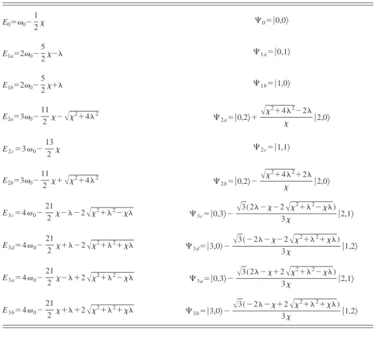
We report in Table I, in algebraic form, the eigenvalues and eigenvectors for the matrix n

具

ns,na兩H0⫹H2⫹兩ns

⬘

,na

⬘典

n

truncated at first order in ␹ and ␭ for n_s⫹n_a⫽n_s

⬘

⫹n_a

⬘

⫽0,1,2,3. The dynamical problem has been examined by many authors,24 –27with the aim of proving the equivalence of the normal-mode description versus the local-mode de-scription. The expressions reported in the Table satisfy the relations兩E1a⫺E1b兩⬎兩E2a⫺E2c兩⬎兩E3c⫺E3d兩 for any value

␹⬎0 and ␭⫽0. It is well known24 _{that when ␭⬍␹, the two}

lowest eigenvalues within each manifold (E2a, E2cand E3c, E3d here兲 become nearly degenerate with increasing total

quantum number, in systems consisting of two identical os-cillators.

Consideration of the eigenvectors of Table I at zeroth order in␭ and␹gives also the right combinations respecting the symmetry of the two identical CH oscillators. Using the appropriate expressions of the harmonic-oscillator wave functions37 ␾i(qi) substituted in 兩ns,na

典

n⫽␾s(qs)␾a(qa),

and considering the coordinate transformation, at zeroth or-der in ␧, from normal coordinates (qs,qa) to local

coordi-nates (⌬lI,⌬lII) we obtain the following correspondence at

zero order: ␺2a⫽共2兲⫺1/2共兩0,2

典

n⫹兩2,0

典

n)⫽共2兲⫺1/2共兩0,2

典

ᐉ⫹兩2,0

典

ᐉ), ␺2b⫽兩1,1

典

n⫽共2兲⫺1/2共兩0,2

典

ᐉ⫺兩2,0

典

ᐉ), ␺3c⫽共1/2兲兩0,3

典

n⫹共31/2/2兲兩2,1

典

n ⫽共2兲⫺1/2_共兩0,3

_典

ᐉ⫺兩3,0

典

ᐉ), ␺3d⫽共1/2兲兩3,0

典

n⫹共31/2/2兲兩1,2

典

n ⫽共2兲⫺1/2_共兩0,3

_典

ᐉ⫹兩3,0

典

ᐉ),

兩v1,v2

典

ᐉ⫽␾1(⌬lI)␾2(⌬lII) being local-mode harmonic

wave functions. This means that the two lowest-energy states in each (ns⫹na) manifold are local modes, the involvement

of both coordinates lI and lII being required by

symmetry.25–27 The above relations, providing the local quantum-number–normal-quantum-number correspondence, are correct only at zeroth order in␧ since the transformations

T₁ and T₂ applied on the Hamiltonian imply coordinates transformations too.

III. DETERMINATION OF DIPOLE TRANSITION MOMENTS

We have modeled the operators of electric dipole mo-ment␮ˆ and magnetic dipole moment mˆ in a valence-optical approach; accordingly, they are determined only by individual-bond electric dipole moments, which have been

considered to depend on coordinates and momenta at second order.38 – 41The electric dipole moment␮ˆ , in this approxima-tion, is given by ␮ᠬ ⫽兺i␮ᠬi(⌬ᐉi), and for each bond i we

assume ␮ᠬi共⌬ᐉ兲⫽␮ᠬi 0_⫹␧⳵␮ᠬi ⳵ᐉi

冏

₀ ⌬ᐉi⫹␧2 ⳵2_␮ᠬ i ⳵ᐉi 2

冏

0 ⌬ᐉi 2_{, 共10兲}

with no contributions from cross-terms ⳵␮ᠬi/⳵ᐉj兩0 with i⫽ j. This simplifying assumption easily allows one to use

electro-optical parameters derived from absorption overtone spectroscopy,34,35 but may be eventually dropped if one wants to use the parameters of more advanced calculations. As is usual in overtone spectroscopy, in our HCCH fragment we consider just the CH bond dipole moments and we ignore the CC bond contribution: then, the index i runs from I to II 共we use Roman numbers for bonds and Arabic numbers for orders of approximation兲. In order to apply the perturbative approach illustrated above we need to work in normal coor-dinates, the dipole moment being

␮ᠬ ⫽␮ᠬ0_⫹␧

兺

␣ ␮ᠬ␣q␣⫹␧

2 1

2

兺

␣,␤ ␮ᠬ␣␤q␣•q␤

⫽␮ᠬ0⫹␧␮ᠬ1⫹␧2␮ᠬ2. 共11兲

Considering the general relation between normal and local coordinates, one obtains37,38

␮ᠬ_␣⫽_⳵⳵␮_qᠬ␣冏 0 ⫽

兺

i ⳵␮ᠬi ⳵ᐉi

冉

兺

A s ᠬiA•tᠬA␣

冊

, 共12兲 s

ᠬiA being the Wilson37vector relating internal coordinates to

Cartesian displacements and tᠬA␣ being given in Appendix A.

Referring to the molecular fragment of Fig. 1, the trans-formations relating CH-stretching internal coordinates to di-mensionless normal ones are simply

qa⫽␣a

冑

m/2共⌬ᐉI⫺⌬ᐉII兲, qs⫽␣s

冑

m/2共⌬ᐉI⫹⌬ᐉII兲,

where ␣i are the coefficients allowing one to go from the

usual normal coordinates to mass-weighted ones, reported in Eq. 共A4兲 of Appendix A, and m is the reduced mass of the CH bond. Since⳵␮ᠬ_i/⳵ᐉ_i兩₀are identical in magnitude for the two CH bonds, due to the C₂ symmetry, and since they are assumed to be directed along the bonds, i.e., ⳵␮ᠬ_i/⳵ᐉ_i兩₀ ⫽⳵␮/⳵ᐉ兩₀uˆ_i(uˆ_ibeing the unit vector of bond i, i⫽I,II), the coefficients of Eq. 共11兲 as functions of valence optical pa-rameters⳵␮/⳵ᐉ兩0 and⳵2␮/⳵ᐉ2兩0 are

␮ᠬ_␣⫽_⳵⳵␮ᠬ q␣冏₀⫽ ⳵␮ ⳵ᐉ

冏

₀ uˆI⫾uˆII

冑

2m␣_␣ 共⫹ if ␣⫽s,⫺ if ␣⫽a兲 共13兲 and

TABLE I. Analytical expressions of eigenvalues and unnormalized eigenvectors of the matrix 具ns,na兩H0

⫹H2⫹兩ns⬘,na⬘典for ns⫹na⫽ns⬘⫹na⬘⫽0, 1, 2, 3. The matrix was first truncated to first order in ␭ and␹, and then

it was diagonalized. For the notation, see text; the first quantum number refers to the symmetric mode s; the second one refers to the antisymmetric mode a.

E0⫽␻0⫺ 1 2␹ ⌿0⫽兩0,0典 E1a⫽2␻0⫺ 5 2␹⫺␭ ⌿1a⫽兩0,1典 E1b⫽2␻0⫺ 5 2␹⫹␭ ⌿1b⫽兩1,0典 E2a⫽3␻0⫺ 11 2 ␹⫺冑␹ 2_⫹4␭2 ⌿2a⫽兩0,2典⫹ 冑␹2_⫹4␭2_⫺2␭ ␹ 兩2,0典 E2c⫽3␻0⫺ 13 2 ␹ ⌿2c⫽兩1,1典 E2b⫽3␻0⫺ 11 2 ␹⫹冑␹ 2_⫹4␭2 ⌿2b⫽兩0,2典⫺ 冑␹2_⫹4␭2_⫹2␭ ␹ 兩2,0典 E3c⫽4␻0⫺ 21 2 ␹⫺␭⫺2冑␹ 2_⫹␭2_⫺␹␭ ⌿3c⫽兩0,3典⫺ 冑3共2␭⫺␹⫺2冑␹2_⫹␭2_⫺␹␭兲 3␹ 兩2,1典 E3d⫽4␻0⫺ 21 2 ␹⫹␭⫺2冑␹ 2_⫹␭2_⫹␹␭ ⌿3d⫽兩3,0典⫺ 冑3共⫺2␭⫺␹⫺2冑␹2_⫹␭2_⫹␹␭兲 3␹ 兩1,2典 E3a⫽4␻0⫺ 21 2 ␹⫺␭⫹2冑␹ 2_⫹␭2_⫺␹␭ ⌿3a⫽兩0,3典⫺ 冑3共2␭⫺␹⫹2冑␹2_⫹␭2_⫺␹␭兲 3␹ 兩2,1典 E3b⫽4␻0⫺ 21 2 ␹⫹␭⫹2冑␹ 2_⫹␭2_⫹␹␭ ⌿3b⫽兩3,0典⫺ 冑3共⫺2␭⫺␹⫹2冑␹2_⫹␭2_⫹␹␭兲 3␹ 兩1,2典

␮ᠬ_␣␣⫽⳵ 2_␮ᠬ ⳵q_␣2

冏

0 ⫽⳵ 2_␮ ⳵ᐉ2

冏

0 uˆ_I⫹uˆ_II 2m␣_␣2 共␣⫽s,a兲, 共14兲 ␮ᠬ_␣␤⫽ ⳵ 2_␮ᠬ ⳵q_␣⳵q␤冏 0 ⫽⳵ 2_␮ ⳵ᐉ2

冏

0 uˆI⫺uˆII 2m␣_␣␣_␤, ␣ different from ␤. 共15兲 For the total magnetic dipole moment mᠬ , we adopt the bond dipole valence optical approach, as described in Refs. 39 and 40:

mᠬ ⫽ 1

2c

兺

i 共rᠬAi⫻␮ᠬ˙i⫹␮

ᠬi⫻rᠬ˙Bi兲, 共16兲

where Aiand Biare the two atoms defining bond i. Referring

to the chiral fragment of Fig. 1, let us take the coordinate origin in CI; in the hypothesis that rCIIis fixed and that uᠬi

and␮ᠬ˙iare always parallel to the fixed direction uˆigiven by

the equilibrium orientation of bond i, one obtains

mᠬ ⫽ 1

2crᠬCII⫻␮ᠬ˙II. 共16⬘兲

Analogously to the electric dipole moment, we need an ex-pression of mᠬ as a function of normal coordinates and/or conjugated momenta: mᠬ ⫽mᠬ0⫹␧

兺

␣ ␰ ᠬ␣_p ␣⫹␧2

兺

␣,␤ ␰ ᠬ_␣␤

冉

q␣•p␤⫹p␤•q␣ 2

冊

⫽mᠬ0⫹␧•mᠬ1⫹␧2mᠬ2. 共17兲

Since q˙_␣⫽␣_␣2•p_␣ 共see Appendix A兲, ␰ᠬ␣_⫽1 2crᠬCII⫻ ⳵␮ᠬII ⳵ᐉII

冉

兺

A s ᠬ2A•tᠬA␣

冊

•␣_␣ 2 ⫽⫾_2c1 rᠬCII⫻

冉

⳵␮ ⳵ᐉ

冊

₀ ␣␣

冑

2muˆII, ⫹ if␣⫽s, ⫺ if␣⫽a, 共18兲 ␰ᠬ␣␤⫽⫾ 1 2crᠬCII⫻

冉

⳵2_␮ ⳵ᐉ2

冊

0 ␣␤

2m␣_␣uˆII,⫹if␣⫽␤,⫺if␣⫽␤. 共19兲 The rotational strength

R⫽Im共n

具

⌿0兩␮ᠬ 兩⌿f

典

n•n

具

⌿f兩mᠬ兩⌿0

典

n兲 共20兲

has been demonstrated to be origin independent for the fun-damental transition 0→1.39The same invariance needs to be proved for the overtone and combination transitions. Dipole strengths and rotational strengths are obtained from the tran-sition moments evaluated on the perturbed wave functions ⌿⫽T1⫺1T2⫺2U⫺1兩ns,na

典

n. Alternatively, one may apply Van

Vleck contact transformations directly on operators; we can easily construct␮⫹and m⫹ from Eqs.共2兲 and 共6兲, with the help of the algebraic manipulator code:

␮ˆ⫹_{⫽T2•T1•␮}ˆ_•T1⫺1_•T2⫺1 ⫽␮ˆ₀⫹_⫹␧␮ˆ₁⫹_⫹␧2_␮ˆ 2 ⫹_⫹␧3_␮ˆ 3 ⫹_⫹␧4_␮ˆ 4 ⫹_, mˆ⫹_⫽T2•T₁•mˆ•T₁⫺1•T₂⫺1 ⫽mˆ0⫹⫹␧mˆ1⫹⫹␧ 2_mˆ 2 ⫹_⫹␧3_mˆ 3 ⫹_⫹␧4_mˆ 4 ⫹_.

Considering homologous terms in␧ and being the initial op-erators ␮ and m in Eqs. 共11兲 and 共17兲 of the form fˆ⫽ fˆ0

⫹␧• fˆ1⫹␧2• fˆ2, with f0 independent of p and q, the

trans-formations共2兲 and 共6兲 can be written

fˆ₀⫹⫽ fˆ0, fˆ₁⫹⫽ fˆ₁, fˆ₂⫹⫽ fˆ2⫹ibS1, fˆ1c, 共21兲 fˆ3⫹⫽i关S1, fˆ2兴⫺ 1 2关S1,关S1, fˆ1兴兴⫹i关S2, fˆ1兴, fˆ₄⫹⫽⫺1 2关S1,关S1, fˆ2兴兴⫺ i 6关S1,关S1,关S1, fˆ1兴兴兴 ⫹i关S2, fˆ2兴⫺关S2,关S1, fˆ1兴兴.

In the calculations presented in the next paragraph we keep terms up to fourth order. The expressions of the transformed operators, as functions of the electric and magnetic dipole moment coefficients␮ᠬ_␣,␮ᠬ_␣␤,␰ᠬ␣,␰ᠬ_␣␤ and of the transforma-tion coefficients Si jkand Si jkl, are very long. We report them

in Appendix B, Eqs. 共B1兲–共B6兲, truncated at third order. In Appendix C we report the proof of the origin independence of the rotational strengths obtained with the transformed op-erators ␮ˆ⫹ and mˆ⫹, for the first two overtone transitions. With the aid of the algebraic manipulator used to build ␮ˆ⫹ and mˆ⫹, one can easily substitute numerical values for ⳵␮/⳵ᐉ兩₀ and⳵2_␮/⳵ᐉ2_兩

0 and␻0, ␹, and ␭, and one can

cal-culate numerically dipole and rotational strengths for HCCH fragments with different dynamical and electrical character-istics. Before considering the specific numerical example treated in the following paragraph, a few comments on the analytical findings are worthwhile.

The transition moments based on harmonic uncoupled-oscillator wave functions 兩ns,na

典

n depend on the

electroop-tical parameters␮_␣, ␮_␣␤, ␰_␣, ␰_␣␤ and on the S_{i jk} and S_{i jkl} coefficients. Of course, first-order terms in ␧ contribute only to 0→1 transitions by linear electrical coefficients 共with mi-nor corrections from all successive odd-order terms兲, ␧2 terms contribute only to 0→2 transitions by linear electrical terms multiplied by Si jk, and quadratic electrical terms共and

minor corrections from successive even-order terms兲. The 0→3 transitions have contributions from ␧3 terms, linear electrical terms are multiplied by Si jklor by Si jk•Si⬘j⬘k⬘, and

quadratic terms are multiplied by Si jk. The 0→4 transitions

derive from␧4 terms. From Appendix A we know that in the approximation ␻s⯝␻a⯝␻0 the coefficients of the

generat-ing functions are of the followgenerat-ing orders of magnitude:

In Table II we report the leading term in

冑

␹/␻for dipole and rotational strengths. These approximate analytical ex-pressions give an estimate of absorption and VCD spectra for the fundamental transitions (n⫽ns⫹na⫽1), as well as for

the first two overtone regions (n⫽2,3). The limitations of these approximations will be tested in the numerical example given in the next section. A few observations can be made based on the results of Table II. As long as electrical anhar-monicity can be ignored, as, e.g., in the fixed partial charge approximation,38 the dipole strengths for the first overtone region (ns⫹na⫽2) are smaller than those for the

fundamen-tal region by a factor of␹/␻and those for the second over-tone region (ns⫹na⫽3) by a factor of (␹/␻)2. As a

conse-quence, a decrease in intensity of nearly two orders of magnitude at each overtone order 共with reasonable CH stretching parameter values as those used in the next section兲 is to be expected. This rapid decrease is indeed observed only from fundamentals to first overtones; for successive overtones, there is a less marked decrease and this has been attributed to the fact that electrical anharmonicity is important.34 –36 A further consequence of the hypothesis of zero electrical anharmonicity is that the two transitions at lowest frequency within each manifold are the only ones predicted to be observable: moreover, they have nearly equal absorption intensity and opposite rotational strengths. Deal-ing with the ⌬n⫽3 region, one sees from Table II that the two lowest-lying transitions are so close as to make any ob-servation of rotational strength impossible.

In conclusion, the presence of electrical anharmonicity is necessary to ensure the right decrease of intensities among different manifolds and confirms the predominance of the two low-frequency transitions within the same manifold.

Rough estimates of the intensity parameters are obtained introducing the quantity␥⫽(1/2␲)

冑

hNA/2c␻0共␥⬵0.075 Å

when ␻0⫽3000 cm⫺1). We have ␮␣⬇␥⳵␮_⳵ᐉ

冏

0 , ␰␣⬇ប⫺1␲rCC␥ ⳵␮ ⳵ᐉ

冏

₀␻0, ␮␤␣⬇␥2⳵ 2_␮ ⳵ᐉ2

冏

0 , ␰_␣␤⬇ប⫺1␲rCC␥2 ⳵2_␮ ⳵ᐉ2

冏

0 ␻0.

Regardless of the electro-optical parameters adopted, ⳵␮/⳵ᐉ兩0 and ⳵2␮/⳵ᐉ2兩0, and taking rCC⫽1.54 Å, ␻0

⫽3000 cm⫺1_{, one hasR}

0_→v⫽1.4⫻10⫺4•D0_→v. This gives

a dissymmetry factor G⫽4R/D⫽4␲rCC␻0⬵6⫻10⫺4

in-dependently of v, as experimentally observed thus far in most cases.3,42

Let us make a final comment regarding the number of transformations needed in the Van Vleck procedure. The Hamiltonian of Eq. 共1兲 has been diagonalized to second or-der in␧, and the use of zeroth order eigenfunctions is justi-fied since the corrections are taken into account on the op-erators. In general the transformed Hamiltonian

H⫹⫽H₀⫹⫹␧•H₁⫹⫹␧2•H⫹₂⫹␧3•H₃⫹⫹␧4•H₄⫹⫹¯ TABLE II. Final states␺fat zero order in␹and␭, approximate transition frequencies␻f⫺␻iin the hypothesis␭Ⰶ␹, and principal terms in冑␹/␻of dipole

strengthsD and rotational strengths R from the ground state 兩0,0典 towards the final states␺ffor ns⫹na⫽1, 2, 3. For the definition of symbols used, see text.

␺f ␻f-␻i D R 兩0,1典 ␻0⫺2␹⫺␭ ␮ᠬa 2 2 ⫹¯ ប 2␮ᠬa•␰ᠬa⫹¯ 兩1,0典 ␻0⫺2␹⫹␭ ␮ ᠬs 2 2 ⫹¯ ប 2␮ᠬs•␰ᠬs⫹¯ 1 冑2共兩0,2典⫹兩2,0典) 2␻0⫺6␹⫺ 2␭2 ␹ 1 16

冉

␮ᠬaa⫹␮ᠬss⫺2

冑

␹ ␻ ␮ᠬs

冊

2 ⫹¯ ប₈

冉

␮ᠬaa⫹␮ᠬss⫺2

冑

␹ ␻ ␮ᠬs

冊

•

冉

␰ᠬaa⫹␰ᠬss⫺2

冑

␹ ␻ ␰ᠬs

冊

⫹¯ 兩1,1典 2␻0⫺6␹ 1 4

冉

␮ᠬsa⫺

冑

␹ ␻ ␮ᠬa

冊

2 ⫹¯ ប₄

冉

␮ᠬsa⫺

冑

␹ ␻ ␮ᠬa

冊

•

冉

␰ᠬs a ⫹␰ᠬa s ⫺2

冑

_{␻ ␰}␹ᠬa

冊

⫹¯ 1 冑2共兩0,2典⫺兩2,0典) 2␻0⫺4␹⫹ 2␭2 ␹ 1 16共␮ᠬaa⫺␮ᠬss兲 2_⫹¯ ប 8共␮ᠬaa⫺␮ᠬss兲•共␰ᠬaa⫺␰ᠬss兲⫹¯ 1 2兩0,3典⫹ 冑3 2 兩2,1典 3␻0⫺12␹⫺ 3␭2 4␹ 3 4 ␹ ␻

冉

␮ᠬsa⫺ 2 3

冑

␹ ␻ ␮ᠬa

冊

2 ⫹¯ ប3₄␹_␻

冉

␮ᠬsa⫺ 2 3

冑

␹ ␻ ␮ᠬa

冊

•

冉

3 2共␰ᠬs a_⫹␰ᠬ a s_兲⫺2

冑

␹ ␻ ␰ᠬa

冊

⫹¯ 1 2兩3,0典⫹ 冑3 2 兩1,2典 3␻0⫺12␹⫺ 3␭2 4␹ 3 4 ␹ ␻

冋

1 2共␮ᠬss⫹␮ᠬaa兲⫺ 2 3

冑

␹ ␻ ␮ᠬs

册

2 ⫹¯ ប3_4␻␹

冉

1₂共␮ᠬss⫹␮ᠬaa兲⫺ 2 3

冑

␹ ␻ ␮ᠬs

冊

•

冉

3 2␰ᠬaa⫺2

冑

␹ ␻ ␰ᠬs

冊

⫹¯ 冑3 2 兩0,3典⫺ 1 2兩2,1典 3␻0⫺8␹⫺2␭⫹ 3␭2 4␹ 0 0 冑3 2 兩3,0典⫺ 1 2兩1,2典 3␻0⫺8␹⫹2␭⫹ 3␭2 4␹ 1 16 ␹ ␻共␮ᠬaa⫺␮ᠬss兲 2_⫹¯ ប 3 16 ␹ ␻共␮ᠬaa⫺␮ᠬss兲•共␰ᠬaa⫺2␰ᠬss兲⫹¯

contains terms in ␧3,␧4,... which are not diagonal and can be diagonalized by introducing further contact transforma-tions generated by S3,S4,... . These generating functions

give rise to further corrections on the operators␮ˆ and mˆ . Our treatment has been coherently developed up to third order in ␧ for ␮ˆ and mˆ . Indeed, from Eq.共21兲 one observes that S1

gives origin to corrections in␧2 and S2to corrections in␧3.

If one imagines to carry on the perturbative treatment with a function S3, the third-order term will not be corrected

any-more (␮₃⫹⫹⫽␮₃⫹), while the fourth-order term will become ␮4⫹⫹⫽␮4⫹⫹i关S3,␮1兴. This is the reason why our treatment

can be considered satisfactory for the⌬v⫽1,2,3 transitions and needs to be improved for⌬v⭓4. Since the contribution of electrical anharmonicity (␮₂ term兲 is greater than the␮₁ term,35we expect our results to be quite acceptable also for ⌬v⫽4 in the numerical case we examined, even without making the transformation S3; of course, this would not be

the case with ⳵2_␮ᠬ /_⳵ᐉ2_兩

0⬇0. The analytical expressions for

⌬v⫽4 do not allow any further insight into the description of the normal-mode to local-mode transition, and we do not report them here.

IV. NUMERICAL EXAMPLE

In this section we present a numerical example where we have used the complete expressions of operators␮ˆ and mˆ to fourth order in order to calculate intensities and rotational strengths for a case representing aliphatic CH’s. The opera-tors, due to all the relations given in Appendix A, ultimately depend only on the mechanical parameters␻₀,␹, and␭ and on the electrical parameters ⳵␮/⳵ᐉ兩0 and ⳵2␮/⳵ᐉ2兩0. The

values for those parameters used in the calculation are given in Table III. Here␻0 and␹ values refer to no specific

mol-ecule but are well representive of aliphatic CH’s. Also, ⳵␮/⳵ᐉ兩0 and ⳵2␮/⳵ᐉ2兩0 have been taken from a previous

work by our group on overtone absorption intensities,35 where overtone experimental absorption intensity data were used to parametrize the bond electric dipole moment, ex-pressed through a linear plus a quadratic dependence on the bond stretching coordinate. In that work, as in many other well-known papers34 –36 in the literature, the importance of electrical anharmonicity had been pointed out, and different functional dependences have also been proposed. In Table III

TABLE III. Values for the mechanical CH bond parameters␻0,␹,␭ and for the electric bond dipole moment

parameters⳵␮/⳵ᐉ兩0,⳵2␮/⳵ᐉ2兩0employed in the numerical example of Table IV共for the latter parameters see

Ref. 31兲. We also report the corresponding normal-mode parameters derived as described in Appendix A.

␻0⫽3000 cm⫺1

␹⫽60 cm⫺1 _{⳵␮/⳵ᐉ兩}

0⫽⫺0.143e

␭⫽20 cm⫺1 _⳵2_␮/⳵ᐉ2_兩

0⫽⫺0.485e/Å

Parameters derived from the preceding ones

␻s 3020 cm⫺1 ␻a 2980 cm⫺1 兩␮s兩⫽0.872⫻10⫺19esu cm ប兩␰s兩⫽0.706⫻10⫺23esu cm Ksss ⫺210.1 cm⫺1 兩␮a兩⫽0.620⫻10⫺19esu cm ប兩␰a兩⫽0.702⫻10⫺23esu cm Ksaa ⫺638.7 cm⫺1 兩␮ss兩⫽0.110⫻10⫺21esu cm ប兩␰a s 兩⫽0.865⫻10⫺26_{esu cm} Kssss 17.3 cm⫺1 兩␮aa兩⫽0.112⫻10⫺21esu cm ប兩␰s a 兩⫽0.854⫻10⫺26_{esu cm}

Kaaaa 17.7 cm⫺1 兩␮sa兩⫽0.785⫻10⫺22esu cm ប兩␰aa兩⫽0.859⫻10⫺26esu cm

Kssaa 105 cm⫺1 ប兩␰ss兩⫽0.859⫻10⫺26esu cm

TABLE IV. Final states, transition frequencies␻, dipole strengthsD, and rotational strengths R calculated for the fundamental and first three overtones in the numerical case defined by the parameters reported in Table III on the basis of the perturbative treatment, with no further approximation共columns 1–4兲. In columns 5 and 6 the corresponding approximated values for the fundamental and first two overtones have been obtained according to the results of Table II. Final state U⫺1兩ns,na典 ␻共cm⫺1兲 D 共esu2cm2兲 R 共esu2cm2兲 D 共esu2cm2兲 R 共esu2cm2兲

共0,1兲 2862 0.23⫻ 10⫺38 ⫺0.19 ⫻ 10⫺42 0.19⫻ 10⫺38 ⫺0.16 ⫻ 10⫺42 共1,0兲 2903 0.46⫻ 10⫺38 0.19⫻ 10⫺42 0.38⫻ 10⫺38 0.16⫻ 10⫺42 0.88共0,2兲⫹0.47共2,0兲 5632 0.29⫻ 10⫺40 0.18⫻ 10⫺44 0.37⫻ 10⫺40 0.31⫻ 10⫺44 共1,1兲 5644 0.16⫻ 10⫺40 ⫺0.21 ⫻ 10⫺44 0.19⫻ 10⫺40 ⫺0.31 ⫻ 10⫺44 0.47共0,2兲⫺0.88共2,0兲 5780 0.29⫻ 10⫺41 0.20⫻ 10⫺45 0.14⫻ 10⫺48 0 0.64共0,3兲⫹0.77共2,1兲 8280 0.16⫻ 10⫺41 ⫺0.41 ⫻ 10⫺45 0.50⫻ 10⫺42 ⫺0.12 ⫻ 10⫺45 0.39共3,0兲⫹0.92共1,2兲 8281 0.33⫻ 10⫺41 0.41⫻ 10⫺45 0.99⫻ 10⫺42 0.12⫻ 10⫺45 0.64共2,1兲⫺0.77共0,3兲 8497 0.37⫻ 10⫺43 ⫺0.96 ⫻ 10⫺47 0 0 0.92共3,0兲⫺0.39共1,2兲 8579 0.42⫻ 10⫺43 0.55⫻ 10⫺47 0.27⫻ 10⫺50 ⫺0.26 ⫻ 10⫺52 0.44共0,4兲⫹0.28共4,0兲⫹0.85共2,2兲 10802 0.25⫻ 10⫺42 ⫺0.52 ⫻ 10⫺46 0.62共3,1兲⫹0.78共1,3兲 10802 0.14⫻ 10⫺42 0.55⫻ 10⫺46 0.41共4,0兲⫺0.86共0,4兲⫹0.31共2,2兲 11149 0.21⫻ 10⫺44 ⫺0.46 ⫻ 10⫺48 0.62共1,3兲⫺0.78共3,1兲 11182 0.18⫻ 10⫺44 0.58⫻ 10⫺48 0.26共0,4兲⫹0.87共4,0兲⫺0.42共2,2兲 11336 0.20⫻ 10⫺45 ⫺0.44 ⫻ 10⫺49

we also give the corresponding values of the normal-mode anharmonic force constants Ki jl, Ki jkl and of the

normal-mode electric and magnetic dipole moment coefficients␮_␣, ␮␣␤, ␰␣, ␰␣␤, according to the relations in Appendix A and to Eqs. 共13兲–共15兲 and 共18兲, 共19兲. In Table IV we report the results for frequencies, dipole strengths, and rotational strengths of the transitions from the ground state to eigen-states of the fourth-order Hamiltonian H⫹ up to the third overtone, with inclusion of the DD resonance, that is to say, the states U⫺1兩ns,na

典

n 共with ns⫹na⫽4). In Table IV we

also compare the numerical results obtained by running the perturbative treatment to the best of the present approxima-tion with the results obtained with the approximate analytical derivations of Table II: the approximate formulas give the correct orders of magnitude only for the two most intense transitions at each overtone order. This is due to the approxi-mation␻_s⬵␻_a, which is not acceptable for the other tran-sitions.

The results presented in Table IV are quite satisfactory. First of all, the decrease of overtone absorption intensities by two orders of magnitude in going from fundamentals to first overtones and by one order of magnitude at each successive overtone has been observed also in CD for some terpenes and cyclic ketones.3 These observations are matched by our numerical results of Table IV for⌬n⫽1,2,3,4. The electrical parameters are such that ⳵2␮/⳵ᐉ2兩0 starts to contribute at

⌬n⫽2, and at this overtone order its contribution is in part canceled by the contribution of the linear term, thus explain-ing the more rapid decrease of the first overtone with respect to the others.

Furthermore, we observe that the highest absorption in-tensities within each manifold are due to two nearly degen-erate vibrations at very low frequency共not yet degenerate at ⌬n⫽2). As can also be seen from Tables I and II for ⌬n ⫽2, ⌬n⫽3, both these two states are linear symmetric com-binations of states兩ns,na

典

ncoupled via DD interactions. All

other vibrational states correspond to dipole strengths at least one order of magnitude lower. From our calculations we see that the same happens for rotational strengths, but at each overtone order the two degenerate states have opposite signs and so they tend to cancel one another.

The results obtained here for dipole strengths are exactly as expected in the local mode picture: considering the two CH bonds as ‘‘local’’ anharmonic oscillators of quantum states兩v_I,vII

典

ᐉ,

28,34_{both from classical and quantum studies,}

one obtains that overtones 兩v,0

典

_ᐉ 共with v⫽vI⫹vII) have

lower frequencies and higher intensities than combination states, so that the bands usually observed in near-infrared 共NIR兲 spectroscopy 共in absence of Fermi resonances兲 are due to nearly degenerate states兩v,0

典

_ᐉ⫾兩0,v

典

_ᐉ. If one considers these states in Eq.共20兲 as defining rotational strengths, in the valence bond approach of Eqs.共10兲 and 共16兲, one has R⫽Im共ᐉ

具

0,0兩␮ᠬI兩共v,0兲⫾共0,v兲

典

ᐉ•ᐉ

具

共v,0兲⫾共0,v兲兩mᠬII兩0,0

典

ᐉ兲

⫽⫾Im

冉

ᐉ

具

0,0兩␮ᠬI兩v,0

典

ᐉ• rCC

2c ⫻ᐉ

具

v,0兩␮ᠬ˙II兩0,0

典

ᐉ

冊

,

thus giving origin to rotational strengths of opposite signs.

V. CONCLUSIONS

In this work we have presented the analytical expres-sions of frequencies, dipole strengths, and rotational strengths for the fundamental CH-stretching region and the first two overtone regions in a HCCH chiral fragment with

C2 symmetry. This work has been made possible by the use

of the Van Vleck contact transformation scheme performed by means of an algebraically based computer code. The ex-pressions obtained for the transformed operators in Appendix B and for approximate dipole and rotational strengths in Table II are valid for the most general dipole with quadratic dependence 关see Eqs. 共11兲 and 共17兲兴; they do not require a valence bond optical model. It is only the evaluation of the coefficients of Eqs. 共11兲 and 共17兲 that is based on the coupled-oscillator valence optical hypothesis. Our final nu-merical calculations rely on the assumption of bond-localized mechanical and electrical properties. Despite the approximations made, the analytical dependences on the pa-rameters allow one to gain a deep insight into the normal-mode to local-normal-mode transition and the spectroscopic signa-ture of it. The role of each parameter is well evidenced by the present treatment. As already well known, it is the DD coupling that is essential in generating the eigenstates that reproduce the usually observed local modes at high ⌬v’s. From the expressions obtained for dipole strengths the role of the electrical anharmonicity and the prevalence of low-frequency modes in absorption are well documented. The novelty of this work, however, mostly regards rotational strengths of overtone transitions. The numerical results given in Table IV can be considered to represent well both funda-mental and overtone data for a transition from a normal-mode regime to a local-normal-mode one. For this reason a treatment like the one undertaken here is beyond the two crude simpli-fying starting schemes—that is to say, the normal-mode ap-proach and the local-mode apap-proach. If the two bonds are mechanically identical as imposed here, they give origin to degenerate local modes with rotational strengths of opposite signs. Of course, the prediction that no VCD beyond ⌬v ⫽2 can be observed for an HCCH fragment of the sort ex-amined here, with two identical oscillators, is in some cases against experimental evidence.3 At this point the following assumptions need to be revised in the model:共i兲 the two CH bonds are equivalent, 共ii兲 coupling to other modes such as torsion4 is negligible, and 共iii兲 molecular electric and mag-netic dipole moments are generated by bond electric dipole moments. Anyway, the procedure of Van Vleck transforma-tions adopted here is quite promising also in view of over-coming these limitations: it can be extended to a higher num-ber of oscillators19 and, what is more important for CD, it can be applied to operators␮and m with the general form of Eqs. 共11兲 and 共17兲 without the too severe hypothesis of va-lence bond optical approach. In fact, our experimental find-ings propose both conservative bisignate spectra compatible with coupled bond dipoles, as described here, and noncon-servative monosignate spectra,3 which require a different model for the magnetic moment operator, as already recog-nized and amply done to interpret VCD spectra in the infrared.17,43

ACKNOWLEDGMENTS

We thank the Italian Ministry of Education, University, and Research共MIUR兲, that allowed us to conclude this work through the Grant COFIN2001 for the Project ‘‘Nuovi me-todi teorici e sperimentali per la determinazione della con-figurazione assoluta molecolare.’’

APPENDIX A: DEPENDENCE OFS1ANDS2

COEFFICIENTS ON ANHARMONIC FORCE CONSTANTS

We wish to recall here the dependences of the anhar-monic force constants K_sss, K_saa, K_ssss, K_aaaa, and K_ssaa of Hamiltonian 共1兲 in the text, considering it as the fourth-order approximation of two harmonically coupled symmetry-equivalent Morse oscillators representing two symmetry-equivalent bonds and transformed from bond共local兲 coordinates to nor-mal coordinates, i.e.,

H⫽共p_I2/2m兲⫹共p_II2/2m兲⫹D关1⫺exp兵⫺a共lI⫺l0兲其兴2

⫹D关1⫺exp兵⫺a共lII⫺l0兲其兴 2_⫹K

I,II共lI⫺l0兲共lII⫺l0兲.

共A1兲 We recall the relations between Morse parameters D and a to the mechanical frequency ␻0 and anharmonicity␹:4,24

D⫽␻0 2

/4␹, a⫽

冑

8␲2mc␹/h. 共A2兲

The third and fourth derivatives of the Morse potential evalu-ated at equilibrium are

Klll⫽共⳵3V/⳵l3兲⫽⫺6a3D, Kllll⫽共⳵4V/⳵l4兲⫽14a4D.

共A3兲 The Hamiltonian used in the perturbative treatment is ob-tained by diagonalizing the zeroth-order term, i.e., consider-ing normal modes. The frequencies of the two normal oscil-lators are

␻s⫽␻0⫹␭, ␻a⫽␻0⫺␭,

where␭⫽1

2KI,II/4␲2c2m␻0, with m the reduced mass of the

CH bond. Dimensionless normal coordinates q_␣ are related to the usual ones Q_␣ by q_␣⫽␣_␣Q_␣, where

␣␣⫽关2␲c␻␣/ប兴1/2 共␣⫽s,a兲. 共A4兲

The Hamiltonian used in the perturbative treatment is that of Eq. 共1兲 with coefficients given by

Ksss⫽共6

冑

2m3/2hc兲⫺1␣s⫺3Klll, 共A5a兲

Ksaa⫽共2

冑

2m3/2hc兲⫺1␣s⫺1␣a⫺2Klll, 共A5b兲

Kssss⫽共48m2hc兲⫺1␣s⫺4Kllll, 共A5c兲

Kaaaa⫽共48m2hc兲⫺1␣a⫺4Kllll, 共A5d兲

Kssaa⫽共8m2hc兲⫺1␣s⫺2␣a⫺2Kllll. 共A5e兲

Inserting Eqs. 共A3兲 into Eqs. 共A5兲 and making use of Eq. 共A2兲, one obtains

Ksss⫽⫺

冑

␹␻0 2 2␻_s3/2, Ksaa⫽⫺ 3

冑

␹␻₀2 2␻_s1/2␻a , 共A6a兲 K_ssss⫽7␹␻0 2 24␻s 2, Kaaaa⫽ 7␹␻₀2 24␻a 2, Kssaa⫽ 7␹␻₀2 4␻s␻a . 共A6b兲 The coefficients relating normal coordinates to Cartesian co-ordinates are tᠬIs⫽ 1

冑

2muˆI, tᠬIIs⫽ 1

冑

2muˆII, tᠬIa⫽ 1

冑

2muˆI, tᠬIIa⫽⫺ 1

冑

2muˆII,

where uI and uII are the unit vectors of bonds CIHI and

CIIHII, respectively.

We report here, for sake of completeness, the coeffi-cients of the generating functions S1 and S2:

Ssss_{⫽⫺共2/3兲关K} sss/␻sប3兴, S_sss⫽⫺关Ksss/␻sប兴, Ssaa_{⫽⫺共2/ប}3_兲关K saa/共4␻a 2_⫺␻ s 2_兲兴共␻ a 2_/␻ s兲, S_saa ⫽⫺共2/ប兲关Ksaa/共4␻a 2 ⫺␻s 2 兲兴␻a, S_aas ⫽⫺共1/ប兲关Ksaa/共4␻a 2_⫺␻ s 2_{兲兴共2␻} a 2_⫺␻ s 2_兲/␻ s, S_ssss⫽⫺ 3 16 2Kssss␻s⫺5Ksss 2 ប3_␻ s 2 , S_aaaa⫽⫺ 1 16 6Kaaaa共␻s 3_⫺4␻ s␻a 2_兲⫹K saa 2 _共8␻ a 2_⫺3␻ s 2_兲 ប3_共⫺4␻ a 2_⫹␻ s 2_兲␻ a␻s , S_ssss ⫽⫺ 1 16 10Kssss␻s⫺9Ksss 2 ប␻s 2 ,

S_aaaa ⫽⫺ 1 16 10Kaaaa共␻s 3_⫺4␻ s␻a 2_兲⫹K saa 2 _共8␻ a 2_⫺5␻ s 2_兲 ប共⫺4␻a 2_⫹␻ s 2_兲␻ a␻s , S_ssaa⫽⫺1 8 Kssaa共␻s 4_⫺4␻ s 2_␻ a 2_⫺8␻ s␻a 3_⫹2␻ a␻s 3_兲⫹K saa 2 _共8␻ s␻a 2_⫹2␻ a␻s 2_兲⫹K saaKsss共10␻s␻a 2_⫺␻ s 3_⫹8␻ a 3_⫺2␻ a␻s 2_兲 共⫺4␻a 2 ⫹␻s 2 兲共␻a⫹␻s兲ប3␻s 2 , S_saas ⫽⫺1 8

K_ssaa共3␻_s4⫺12␻_s2␻_a2⫺8␻_s␻_a3⫹2␻_a␻_s3兲⫹K_saa2 6␻_a␻_s2⫹K_saaK_sss共6␻_s␻_a2⫺3␻_s3⫹8␻_a3⫺2␻_a␻_s2兲

ប␻s 2_共⫺4␻ a 2_⫹␻ s 2_兲共␻ a⫹␻s兲 , Sssa a ⫽⫺1₈ ⫻Kssaa共2␻s 4_⫺8␻ s 2_␻ a 2_⫺12␻ s␻a 3_⫹3␻ a␻s 3_兲⫹K saa 2 _共6␻ s␻a 2_⫹4␻ a␻s 2_⫺4␻ a 3_兲⫹K saaKsss共12␻s␻a 2_⫺6␻ s 3_⫹10␻ a 3_⫺7␻ a␻s 2_兲 ប␻a␻s共⫺4␻a 2_⫹␻ s 2_兲共␻ a⫹␻s兲 , S_assa⫽⫺1 8 ⫻Kssaa共2␻s 4 ⫺8␻s 2 ␻a 2_⫺4 ␻s␻a 3_⫹ ␻a␻s 3_兲⫹K saa 2 共2␻s␻a 2 ⫹4␻a␻s 2_⫹4 ␻a 3_兲⫹K saaKsss共12␻s␻a 2 ⫺6␻s 3 ⫹14␻a 3 ⫺5␻a␻s 2_兲 共⫺4␻a 2_⫹ ␻s 2 兲共␻a⫹␻s兲ប3␻s 2 .

APPENDIX B: TRANSFORMED ELECTRIC DIPOLE MOMENT AND MAGNETIC DIPOLE MOMENT OPERATORS UP TO 2ND ORDER

We report here the terms in ␧, ␧2, and ␧3 of the transformed electric dipole moment and magnetic dipole moment operators关see Eqs. 共11兲 and ff. and 共16兲 and ff. in the text兴:

␮ᠬˆ₁⫹_⫽␮ᠬ sqs⫹␮ᠬaqa, ␮ᠬˆ₂⫹_⫽1 2␮ᠬssqs 2_⫹␮ᠬ saqsqa⫹ 1 2␮ᠬaaqa 2_⫹␮ᠬ sប共Sss s q_s2⫹S_aas q_a2⫹Ssaap_a2⫹3Ssssp_s2兲⫹␮ᠬaប共Ssa a qsqa⫹2Ssaapspa兲, ␮ᠬˆ₃⫹_⫽␮ᠬ sa

冉

បSaa s q_a3⫹បS_sss q_s2qa⫹បSsa a q_s2qa⫹2បSsaa 1 2共qsps⫹psqs兲pa⫹3បS sss_p s 2 qa⫹បSsaa 1 2共qapa 2_⫹p a 2 qa兲

冊

⫹␮ᠬaa

冉

2បSsaa 1 2 共qapa⫹paqa兲ps⫹បSsa a _q a 2_q s

冊

⫹␮ᠬss

冉

បSss s _q s 3_⫹បS aa s _q a 2_q s⫹3បSsss 1 2 共ps 2_q s⫹qsps 2_兲⫹បSsaa_q spa 2

冊

⫹␮ᠬa

冉

2បSs saa1 2 共qsps⫹psqs兲pa⫹បSaaa a qa 3_⫹3បS a aaa1 2共qapa 2_⫹p a 2 qa兲⫹បSssa a qs 2 qa⫹បSa ssa ps 2 qa⫹ 1 2ប 2_S aa s Ssa a qa 3 ⫹3₂ប2_Ssss_S sa a p_s2qa⫺ 1 2ប 2_S sa a Ssaa1 2 共pa 2 qa⫹qapa 2_兲⫹1 2ប 2_关共S sa a _兲2_⫹S ss s S_saa 兴q_s2qa⫺2ប2SsaaSss s 1 2共qsps⫹psqs兲pa ⫺2ប2_Ssaa_S aa s _p s 2_q a

冊

⫹␮ᠬs

冉

បSsaa s _q a 2_q s⫹2បSa ssa1 2共qapa⫹paqa兲ps⫹បSsss s _q s 3_⫹ប2_S sa a _S aa s _q a 2_q s⫹3បSs sss1 2 共qsps 2 ⫹ps 2 qs兲⫹ប2共Sss s _兲2_q s 3_⫹បS s saa pa 2 qs⫹ប2Saa s Sss s qa 2 qs⫺ប2Ssa a Ssaapa 2 qs⫺3ប2SsssSsa a 1 2 共qapa⫹paqa兲ps ⫹ប2_Ssaa_S ss s p_a2qs⫺3ប2Sss s Ssss1 2 共ps 2 qs⫹qsps 2_兲

冊

, mᠬˆ₁⫹⫽␰ᠬsps⫹␰ᠬapa, mᠬˆ₂⫹⫽␰ᠬss 1 2 共qsps⫹psqs兲⫹␰ᠬaa 1 2 共qapa⫹paqa兲⫹␰ᠬa s_p sqa⫹␰ᠬs a_p aqs⫹␰ᠬs2Sss s _ប

冉

_2S ss s 1 2 共qsps⫹psqs兲⫹Ssa a 1 2共qapa⫹paqa兲

冊

⫹␰ᠬaប共Ssa a _q spa⫹2Saa s _q aps兲,

mᠬˆ₃⫹⫽␰ᠬs

冉

ប共បSss s S_saa ⫺2S_ssaa 兲1 2共qapa⫹paqa兲qs⫺共Ss sss_⫹3Ssss_S ss s _ប兲បp s 3 ⫹ប共បSaa s S_saa ⫺S_saas ⫺Ss_ssS_aas ប兲q_a2ps ⫺3 2Ssss s ប共qs 2 ps⫹psqs 2 兲⫺关ប2_共S ss s _⫹S sa a 兲Ssaa_⫹S s saa ប兴pa 2 ps⫹ប2共Sss s 兲21 2 共qs 2 ps⫹psqs 2 兲

冊

⫹␰ᠬa

冉

1 2共ប 2_S sa a 共Ssa a _⫺S ss s 兲 ⫺2Sssa s _ប兲q s 2_p a⫹ប共បSss s_S aa s _⫺S saa s _兲共q sps⫹psqs兲qa⫺ 1 2ប共4បSss s _S aa s _⫹2S a ssa_⫹3Ssss_S sa a _ប兲p s 2_p a⫹ 1 2ប

冉

1 2Saa s _S sa a _ប ⫺3Saaa a

冊

_共q a 2 pa⫹paqa 2_兲⫺1 2共2Sa aaa_⫹S ss s S_saa ប兲បp_a3

冊

⫹␰ᠬ_as

冉

ប共⫺2S_sss ⫹S_saa 兲1 2共qsps⫹psqs兲qa⫹ប2Sss s p_s2pa ⫺បSsa a 1 2共qa 2 pa⫹paqa 2 兲

冊

⫹␰ᠬs a

冉

共Sss s _⫺S sa a 兲បqs 2 pa⫺បSaa s 共qsps⫹psqs兲qa⫹Sss s _បp a 3_⫹3បSsss_p aps 2_⫹1 2បSaa s 共paqa 2 ⫹qa 2_p a兲⫹␰ᠬss

冉

3Ssssបps 3_⫹S ss s_បp spa 2_⫺1 2Ssa a _បq s共qapa⫹paqa兲⫹Saa s _បp sqa 2_⫺1 2Sss s _ប共q s 2_p s⫹psqs 2_兲

冊

⫹␰aa2ប共Sss s _p spa 2_⫺S aa s _p sqa 2_兲.

APPENDIX C: ORIGIN INDEPENDENCE OF ROTATIONAL STRENGTHS FOR THE FIRST TWO OVERTONE TRANSITIONS

We have algebraically proved that rotational strengths are origin-independent for the transitions 0→2 and 0→3, un-der the assumption that ␮ᠬ is a series expansion truncated to the second order, as in Eq. 共11兲 in the text, and mᠬ, with respect to a generic origin point O, is given by Eq.共16兲 in the text, i.e.,

mᠬ ⫽ 1

2c

兺

i 共rᠬAi⫻␮ᠬ˙i⫹␮

ᠬi⫻rᠬ˙Bi兲, i⫽I,II. 共C1兲

If the origin is shifted to another point O

⬘

, mᠬ changes by the amount共in the case of two bonds, i⫽I,II):

⌬mᠬ⫽ 1

2c共Yᠬ⫻␮ᠬ˙I⫹Yᠬ⫻␮ᠬ˙II兲, 共C2兲

where Yᠬ ⫽O

⬘

O. One has then to prove that the rotational strength arising out of this term is zero, i.e.,

⌬R⫽Im共

具

0,0兩␮ᠬ⫹兩ns,na

典

•

具

ns,na兩⌬mᠬ⫹兩0,0

典

兲⫽0, 共C3兲

where⌬mᠬ⫹is the transformed operator of Eq.共C2兲: we first have explicitly written an operator ⌬mᠬ in Eq. 共C2兲 in terms of bond parameters⳵␮ᠬi/⳵ᐉi兩0and⳵2␮ᠬi/⳵ᐉi

2_兩

0关see Eqs. 共16兲

and共17兲 and ff. in the text兴. Then we have derived␮ᠬ⫹ and ⌬mᠬ⫹_{according to Eq.共21兲 in the text considering terms up} to␮ᠬ₃⫹and⌬mᠬ₃⫹.

The proof was carried out with the algebraic manipulator

MAPLE for the two manifolds ns⫹na⫽2 and ns⫹na⫽3. It

turns out that every couple of values for ns,na within the

second and third manifold yields⌬R⫽0 identically. We may remark that the U matrix need not be applied, since it does not affect the result, being a linear operator.

1_{T. A. Keiderling and P. J. Stephens, Chem. Phys. Lett. 41, 46共1976兲.} 2

M. Miyazawa, Y. Kyogobu, and H. Sugeta, Spectrochim. Acta, Part A 50, 1505共1994兲.

3_{E. Castiglioni, F. Lebon, G. Longhi, and S. Abbate, Enantiomer 7, 161}

共2002兲; S. Abbate, G. Longhi, L. Ricard, C. Bertucci, C. Rosini, P.

Salva-dori, and A. Moscowitz, J. Am. Chem. Soc. 111, 836共1989兲; S. Abbate, G. Longhi, C. Bertucci, P. Salvadori, S. Boiadjiev, and D. A. Lightner, Enan-tiomer 3, 337共1998兲.

4_{S. Abbate, G. Longhi, and C. Santina, Chirality 12, 180共2000兲.} 5

B. T. Darling and D. M. Dennison, Phys. Rev. 57, 128共1940兲.

6_{L. Halonen, Adv. Chem. Phys. 104, 41共1998兲.}

7_{R. T. Lawton and M. S. Child, Mol. Phys. 37, 1799共1979兲.} 8

E. L. Sibert III, W. P. Reinhardt, and J. T. Hynes, J. Chem. Phys. 77, 3583

共1982兲.

9_{S. Abbate, G. Longhi, K. Kwon, and A. Moscowitz, J. Chem. Phys. 108,}

50共1998兲.

10_{G. Amat, H. H. Nielsen, and G. Tarrago, Rotation-Vibration Spectra of} Polyatomic Molecules共Dekker, New York, 1971兲.

11

H. H. Nielsen, Phys. Rev. 68, 181共1945兲.

12_{H. H. Nielsen, Handbuch der Physik共Springer-Verlag, Berlin, 1959兲, Vol.}

XXXVII/1.

13

M. Herman, Adv. Chem. Phys. 108, 1共1999兲.

14_{T. R. Faulkner, C. Marcott, A. Moscowitz, and J. Overend, J. Am. Chem.}

Soc. 99, 8160共1977兲.

15

C. Marcott, Ph.D. thesis, University of Minnesota, 1979.

16_{C. Marcott, T. R. Faulkner, A. Moscowitz, and J. Overend, J. Am. Chem.}

Soc. 99, 8169共1977兲.

17_{K. L. Bak, O. Bludsky´, and P. Jorgensen, J. Chem. Phys. 103, 10548}

共1995兲.

18_{P. L. Polavarapu, Mol. Phys. 89, 1503共1996兲.} 19

E. L. Sibert III, J. Chem. Phys. 88, 4378共1988兲; X. G. Wang and E. L. Sibert III, ibid. 113, 5384共2000兲.

20

P. Bour and T. A. Keiderling, J. Am. Chem. Soc. 114, 9100共1992兲.

21_{T. B. Freedman, S. J. Cianciosi, N. Ragunathan, J. E. Baldwin, and L. A.}

Nafie, J. Am. Chem. Soc. 113, 8298共1991兲.

22_{L. Laux, Ph.D. thesis, University of Minnesota, 1982.} 23

L. Laux, V. M. Pultz, S. Abbate, H. A. Havel, J. Overend, A. Moscowitz, and D. A. Lightner, J. Am. Chem. Soc. 104, 4276共1982兲.

24

M. S. Child and L. Halonen, Adv. Chem. Phys. 57, 1共1985兲.

25_{K. K. Lehman, J. Chem. Phys. 79, 1098共1983兲.}

26_{I. M. Mills and A. G. Robiette, Mol. Phys. 56, 743共1985兲.} 27_{M. Kellman, J. Chem. Phys. 83, 3843共1985兲.}

28_{B. R. Henry, in Advances in Infrared and Raman Spectroscopy, edited by}

R. J. Clark and R. E. Hester共Elsevier, Amsterdam, 1979兲, Vol. 10, Chap. 4, p. 269.

29_{J. R. Cary, Phys. Rep. 79, 129共1981兲.}

30_{L. E. Fried and G. S. Ezra, J. Chem. Phys. 86, 6270共1987兲.}

31_{For a discussion on convergence see A. Giorgilli, From Newton to chaos:} Modern Techniques for Understanding and Coping with Chaos共Plenum,

New York, 1995兲, p. 21.

32_{Waterloo Maple Inc., computer code}

33_{G. Herzberg, Molecular Spectra and Molecular Structure共Van Nostrand,}

New York, 1950兲, Vol. I.

34_{M. L. Sage and J. Jortner, Adv. Chem. Phys. 47, 293共1981兲.} 35

G. Longhi, G. Zerbi, L. Ricard, and S. Abbate, J. Chem. Phys. 88, 6733

共1988兲.

36_{J-A. Phillips, J. J. Orlando, G. S. Tyndall, and V. Vaida, Chem. Phys. Lett.}

296, 377共1998兲.

37_{E. B. Wilson, Jr., J. C. Decius, and P. C. Cross, Molecular Vibrations}

共McGraw-Hill, New York, 1955兲.

38

T. R. Faulkner, Ph.D. thesis, University of Minnesota, 1976.

39_{J. R. Escribano, T. B. Freedman, and L. A. Nafie, J. Phys. Chem. 91, 46}

共1987兲.

40_{J. R. Escribano and L. D. Barron, Mol. Phys. 65, 327共1988兲.} 41

S. Abbate, L. Laux, J. Overend, and A. Moscowitz, J. Chem. Phys. 75, 3161共1981兲.

42_{The same ratio calculated for G is valid for␰}␣_/␮

␣and␮␤␣/␰␣0␤ . The

presence ofប⫺1in␰is due to the fact that mᠬ in Eq. 共13兲 has been given as a function of p instead of using the dimensionless p/ប. Considering the transition moments of mᠬ , ប disappears, and we can consider that the linear terms go as␲rCC␻0␮␣, the quadratic ones as␲rCC␻0␮␣␤.

43