Chapter 4 HCCI / PCCI COMBUSTION ANALISYS 4.1. INTRODUCTION

Chapter 4

HCCI / PCCI COMBUSTION ANALISYS

4.1. INTRODUCTION

In HCCI combustion operation, fuel is injected and well premixed with air before ignition, thus avoiding fuel-rich regions, which leads to reduction of PM emissions. NOx emissions, which are strongly dependent on gas temperature, are also greatly reduced because the burned gas temperatures are kept relatively low by using lean mixtures.

HCCI combustion implies several difficulties that must be overcome for practical use, such as the controllability of combustion timing, which is an important factor for engine efficiency and exhaust emissions, and the attainment of a mixture with proper characteristics, which is a capital issue of this kind of combustion. In order to actively control the mixture formation process, the DI process is widely adopted in HCCI combustion. Of course, DI must be carefully phased. Early injection is likely to cause significant wall impingement of the injected sprays. Late injection during the compression stroke is likely to cause inhomogeneity of air-fuel ratio inside the cylinder, with local zones of higher fuel concentration that can represent a positive outcome, despite the trite belief that homogeneous combustion implies homogeneous mixture. As a matter of facts, the mixture must only be homogeneous as physical state (all the fuel must be vaporized) and locally homogeneous (the fuel vapor must be locally well mixed with the air). This is what occurs in the case of partially Premixed Charge Compression Ignition (PCCI) combustion, achieved by injecting during compression stroke.

In this section, gasoline HCCI and PCCI combustion have been analyzed to evaluate the influence of some operating conditions (injection timing, fuel amount, air initial temperature etc.) on combustion behavior and emission production. The presence of some air-fuel ratio inhomogeneity, reducing the latency time, can guide the ignition process. However, locally fuel-rich regions can lead to high local temperature and high pollutant emission production. A good compromise could provide interesting results in terms of ignition control with sufficiently low emissions. Results in terms of pressure, heat release rate and emission production have been obtained from numerical and experimental points of view.

The KIVA3V code implemented with two combustion models (Shell-CTC and CHEMKIN) with different accuracies and required computational times, has been used to evaluate the importance of detailed chemistry prediction for low temperature combustion. Being responsible for the in-cylinder mixture distribution, an accurate injection description is undoubtedly essential for combustion simulations of HCCI, and especially for PCCI. In the first part of this study, the

spray models have been tested and validated through available experimental data before proceeding with the combustion simulation.

4.2. NUMERICAL

APPROACH

It is well known that a computational simulation can reduce research and development times. The predictive capabilities of available models complement experimental observations by providing information not available in the experiments. In this section, the simulations are performed using the KIVA3V release 2 code [10] with various improved sub-models developed at the Engine Research Center, University of Wisconsin-Madison. The improved models include spray, atomization, combustion, crevice and pollutant emission models. The LISA breakup model for hollow cone sprays is used to simulate low-pressure atomization of gasoline sprays and the RNG k-ε model is used for predicting turbulence effects. The O’Rourke drop collision model is also present to account for droplets interactions during the injection process. Ignition and combustion processes are simulated using either the Shell auto-ignition model coupled with the Characteristic Time Combustion (CTC) model, or detailed chemistry calculations using CHEMKIN. When the Shell-CTC model is activated, a NOx model [52] based on the extended Zeldovich reactions is used, otherwise a specific reaction pathways is included in the CHEMKIN reaction mechanism. Soot emissions are predicted by a phenomenological soot model using competing formation and oxidation rates. The formation is described by the Nagle-Strickland-Constable (NSC) oxidation model [85]. The parent fuel molecule is used as the species from which the soot forms.

4.2.1. MIT PRF CHEMICAL MECHANISM

When detailed chemistry is used, a skeletal reaction mechanism for primary reference fuel (PRF) with 32 species and 55 reaction [54] is used for the simulation of gasoline HCCI and PCCI combustion. For NOx formation calculation, a simplified NOx formation model, consisting of 4 species and 9 reactions, is obtained from the GRI mechanism [56] and added to the PRF mechanism. It has been confirmed that the additional reactions do not affect the ignition timing predictions. The PRF mechanism coupled with the NOx formation reactions is given in Appendix A.

4.3. SPRAY CHARACTERISTICS VALIDATION

Accurate modeling of spray characteristics is essential for accurate prediction of the mixture distribution in the combustion chamber, especially in PCCI combustion using direct injection. Therefore, the spray model needs to be validated with well-designed experimental measurements before proceeding with combustion simulation.

Table 4.1. Low-pressure injector specifications [18].

Injector type Electronically controlled low- _{pressure common rail injector} Injection pressure 10 MPa

Ambient pressure 0.1 MPa

Nozzle type Pressure swirl atomizer

Spray geometry Hollow cone spray

Spray angle 70˚

Fuel used n-heptane (C7H16)

Injection duration (DOI) 10 msec

Total Fuel injected 94.5 mg

0 1 2 3 4 5 6 7 8 9 10 11 12 13 0.0 0.5 1.0 1.5 2.0 2.5 Nor m aliz ed injec tion r a te Time (msec) Experiment Simulated

Figure 4.1. Experimental and simulated normalized injection rate profile.

Lee and Reitz [15] provided experimental results of spray penetration and drop size distributions for a low-pressure common rail injector. The injection conditions and the nozzle specifications are given in Table 4.1. The experimental and simulated injection profiles are shown in Fig. 4.1. Both are normalized using the average mass flow rate derived from many repeated injections.

The injection inside a cylindrical chamber, with a low-pressure hollow cone spray injector, can be assumed to be an axially symmetric problem. Therefore, a 2-dimensional computational domain of about 5,000 cells has been used for reasonable injection process simulations. Several grid refinements have been tested in order to check the grid-dependency of the results in relation to the computational time. As a result, a grid resolution of about 2.0 x 2.0 mm for every cell has been assumed for this spray model validation.

Figure 4.2 shows a comparison of spray penetration between the measured and predicted results. In the computations, the penetration length is obtained from the 95% accumulated mass distance from the nozzle tip. As expected, as the time increases, the slope of the penetration curve decreases due to the friction between spray droplets and air. From the plot it appears that the models are able to predict penetration lengths in good agreement with experimental measurements.

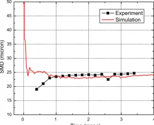
In Fig. 4.3 results in terms of overall SMD (Sauter Mean Diameter) distribution are provided. Discrepancies can be seen in the initial part of the injection where the primary breakup effect takes place. However, the stationary region represents the most interesting part in terms of its influence on the mixture formation inside the engine cylinder and here the numerical results are in good agreement with the experimental ones.

-1 0 1 2 3 4 5 6 0 20 40 60 80 100 120 Pen etratio n (mm ) Time (msec) Experiment Simulation

Figure 4.2. Comparison of experimental and simulated spray penetration length.

10 15 20 25 30 35 40 45 50 SMD (mi cro n) Time (msec) Experiment Simulation 0 1 2 3 4

Figure 4.3. Numerical and experimental comparison of overall SMD distribution.

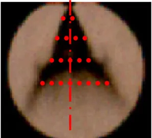
Figure 4.4. Schematic distribution of the measuring points.

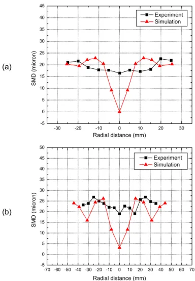
Lee and Reitz [15] also provided local SMD measurements obtained with the Malvern laser technique. In Fig. 4.4 a schematic representation of the choice of the measuring point is reported. Droplet SMD has been measured in different radial locations, at several distances from the injector tip, for multiple injections. In Fig. 4.5, a comparison of predicted and measured results of drop size distribution in the radial direction at two axial locations is shown. The SMD value at each location is obtained by counting all droplets passing that location from the start of injection. The radial SMD distributions are seen to be in fairly good agreement at both locations except for the drop sizes in the spray axis region. However, this was expected because of the swirl-type atomizer. It is well known that at the end of every swirl injection, a certain amount of fuel remains within the sac volume when the injector pin closes, losing its rotational energy. At the beginning of the next injection, this amount of fuel enters the cylinder as soon as the pin starts opening, before the main injection forms the hollow cone spray. This blade of fuel, made up by large droplets, goes along the injector axis and sometimes causes impingement on the piston surface. In the simulation, the droplets near the spray axis cannot be captured because the model assumes an outward-opening swirl atomizer. Thus, the fuel blade is not considered in the model. However the overall effect of the droplets measured in this region is minimal because in the axis region there is a small mass of droplets, despite their large SMD. Therefore, on the whole, the spray model gives a satisfactory representation of the local spray evolution and atomization.

(a) -30 -20 -10 0 10 20 30 -5 0 5 10 15 20 25 30 35 40 45 Experiment Simulation S M D (micro n) Radial distance (mm) (b) -70 -60 -50 -40 -30 -20 -10 0 10 20 30 40 50 60 70 -5 0 5 10 15 20 25 30 35 40 45 50 Experiment Simulation S M D (micron) Radial distance (mm)

Figure 4.5. Comparison of predicted and measured radial SMD distribution of a

hollow cone spray at a two different locations from the injector tip. (a) 20 mm and (b) 40 mm from the injector tip.

For a final validation, shown on Fig. 4.5, predicted spray structure evolutions are compared with experimental high definition images, provided by Sun [16], of the spray pattern of a low pressure swirl atomizer using gasoline fuel. The injection pressure was 4.7 MPa and the ambient pressure was 0.1 MPa. In order to obtain a more accurate prediction of the spray shape, a 3-dimensional cylindrical chamber with 20,000 computational cells was considered. As shown in Fig. 4.6, the predictions capture the transient spray shapes and behaviors excellently, which gives confidence to the spray model used in the study.

1 msec after start of injection 10 cm 2 msec 10 cm 3 msec 10 cm 4 msec 10 cm 5 msec 10 cm

Figure 4.6. Spray shape comparison at several times after SOI. (Left-experiment [16], right-model).

4.4. ENGINE

EXPERIMENTS

Marriott and Reitz [17, 18] performed gasoline HCCI/PCCI combustion tests using a Caterpillar 3401 single-cylinder, four-stroke engine that was originally used for conventional diesel combustion applications. The engine and injector specifications are reported in Tables 4.2 and 4.3, respectively.

Table 4.2. Engine specifications [17,18].

Engine Caterpillar 3401 SCOTE (Single Cylinder Oil Test Engine)

Bore x Stroke 137.2 mm x 165.1 mm

Compression Ratio 16.1:1

Displacement 2.44 liters

Connecting Rod Length 261.62

Squish Height 1.57 mm

Combustion Chamber In-piston Mexican hat with sharp edge crater

Valve-train (4-valve) EVC = -355 degATDC IVC = -143 deg ATDC EVO = 130 deg ATDC IVO = 335 deg ATDC

Table 4.3. Injector specifications [17,18].

Injector Type Delphi Electronically Controlled DI-G Injector

Injection Pressure 10 MPa

Nozzle Type Pressure Swirl atomizer

Spray Geometry Hollow Cone

Spray Angle (included) 70˚

Spray Orientation Coaxial with engine cylinder

Fuel injected Gasoline

Injection duration 3.2 msec

In Fig. 4.7 the major geometrical details of the reference engine are shown. The adopted injector is the same as that used for the spray model validation proposed in the previous section.

Figure 4.7. Caterpillar 3401 SCOTE geometrical details.

4.4.1. OPERATING CONDITIONS

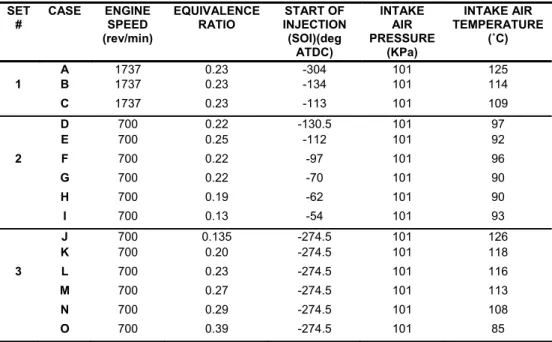
Among the experimental results provided in Refs. 17 and 18, three different sets of operating conditions in 15 different cases ranging from HCCI to PCCI combustion were selected for this study, as described in Table 4.4.

Table 4.4. Experimental Operating Conditions.

SET

# CASE ENGINE SPEED (rev/min)

EQUIVALENCE

RATIO INJECTION START OF (SOI)(deg ATDC) INTAKE AIR PRESSURE (KPa) INTAKE AIR TEMPERATURE (˚C) A 1737 0.23 -304 101 125 1 B 1737 0.23 -134 101 114 C 1737 0.23 -113 101 109 D 700 0.22 -130.5 101 97 E 700 0.25 -112 101 92 2 F 700 0.22 -97 101 96 G 700 0.22 -70 101 90 H 700 0.19 -62 101 90 I 700 0.13 -54 101 93 J 700 0.135 -274.5 101 126 K 700 0.20 -274.5 101 118 3 L 700 0.23 -274.5 101 116 M 700 0.27 -274.5 101 113 N 700 0.29 -274.5 101 108 O 700 0.39 -274.5 101 85

Sets number 1 and 2 contain experiments performed at different engine speeds using different injection timings. The equivalence ratio is constant for set number 1 and is constant for most of set number 2, where it was reduced to avoid too severe stress to the engine structure due to the late-injection operating condition (cases H and I). Finally, the third set of operating conditions is obtained with fixed injection timing and different equivalence ratios.

In the last column in Table 4 it can be seen that a heater was used to create ignitable initial conditions at IVC for the lean mixtures. Auto-ignition of lean gasoline/air mixtures is hard to obtain due to its long ignition delay with naturally aspirated air conditions at room temperature. Therefore, the initial temperature has to be increased to ensure ignition with the compression ratio and speed of the engine considered in this study. Note that the intake gas temperature was also adjusted to avoid severe stress to the engine for the cases with high enough equivalence ratio mixtures (case O).

The range of SOI timings used in these experiments is very wide and covers the range needed for analysis of HCCI and PCCI cases. The equivalence ratio range also covers the usual conditions for these combustion regimes.

4.5. HCCI AND PCCI SIMULATIONS

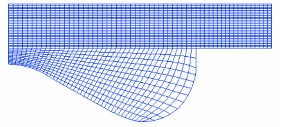
The piston geometry and computational grid used for the simulations are shown in Fig. 4.8. A two dimensional mesh has been used in this study, considering the axial-symmetry of the hollow cone sprays from the centrally-located swirl atomizer. All major geometric dimensions of the experimental combustion chamber, including bore, stroke, bowl volume and squish height have been exactly replicated in the computational grid. The mesh is composed of about 20,000 computational cells at bottom dead center (BDC).

Figure 4.8. Computational grid for HCCI/PCCI simulations.

In order to save computational time and resources, the simulations have been performed from IVC to EVO crank angles, as shown in Table 4.2. However, looking at the Tab. 4.4, it appears that all the cases of set number 3 and a single case of set number 1 have SOI before IVC. In these cases, to avoid the necessity of 3-D moving intake valve computations, the initial mixture composition has been assumed to be homogeneous at the beginning of the simulation. This assumption can be considered adequately safe since the injection timing for these cases is largely advanced compared to IVC. Justification for this approach has been demonstrated by Ra and Reitz [86].

For the Shell-CTC model the standard model constants have been tuned in order to match the ignition delay time and the apparent heat release rate for gasoline fuel. Once tuned, these constants have been kept fixed for all the simulations. In the detailed chemistry model cases, the original set of reaction rate coefficients [54] has been used. It is noteworthy that the computational time required for simulations including detailed chemistry calculation is larger by 50% than the time required from the Shell-CTC combustion model.

4.6. HCCI AND PCCI RESULTS

Results in terms of pressure profiles and apparent heat release rates have been obtained with both the adopted combustion models and compared with experimental data for all the fifteen cases, but only one representative case for every set is shown below for brevity.

In Figs. 4.9, 4.10 and 4.11 the measured and simulated pressure profile and apparent heat release rate (AHRR) for cases C, D and M are compared. AHRR, directly derived from pressure profile, is used in this study to compare numerical and experimental rate of heat release in order to rightly account for the heat transferred to the cylinder wall.

-40 -20 0 20 40 0 1 2 3 4 5 6 7 0 100 200 300 400 500 600 700 800 900 1000 Experiment Shell-CTC CHEMKIN P ressure (MPa ) CAD ATDC A H RR (J/deg) rpm = 1737 eq_ratio = 0.23 c_ratio = 16.1 inj_timing = -113 ca

Figure 4.9. Pressure profile and apparent heat release rate of CASE C.

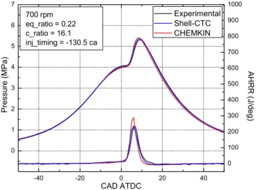
-40 -20 0 20 40 0 1 2 3 4 5 6 7 0 100 200 300 400 500 600 700 800 900 1000 Press u re (MPa) CAD ATDC Experimental Shell-CTC CHEMKIN 700 rpm eq_ratio = 0.22 c_ratio = 16.1 inj_timing = -130.5 ca AHRR (J/ deg )

Figure 4.10. Pressure profile and apparent heat release rate of CASE D.

-40 -20 0 20 40 0 1 2 3 4 5 6 7 0 200 400 600 800 1000 700 rpm eq_ratio = 0.27 c_ratio = 16.1 inj_timing = - 274.5 ca Pr e ssu re (M Pa) CAD ATDC Experiment Shell-CTC CHEMKIN A HRR (J/ deg )

Figure 4.11. Pressure profile and apparent heat release rate of CASE M.

The simulation predictions come out to agree reasonably well with the experimental data. Both the Shell-CTC and detailed chemistry models are able to predict ignition delay, main apparent heat release rate and peak pressure.

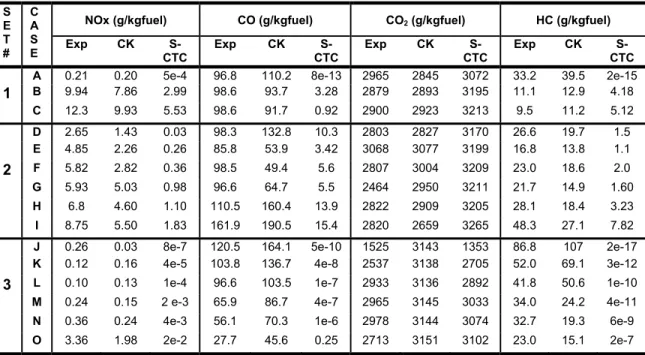
Table 4.5. Pollutant emissions results. The abbreviations ‘Exp’, ’CK’ and ‘S-CTC’ mean experimental, CHEMKIN and Shell-CTC.

NOx (g/kgfuel) CO (g/kgfuel) CO2 (g/kgfuel) HC (g/kgfuel)

S E T # C A S

E Exp CK S-_CTC Exp CK S-_CTC Exp CK S-_CTC Exp CK S-_CTC

A 0.21 0.20 5e-4 96.8 110.2 8e-13 2965 2845 3072 33.2 39.5 2e-15

1 B 9.94 7.86 2.99 98.6 93.7 3.28 2879 2893 3195 11.1 12.9 4.18 C 12.3 9.93 5.53 98.6 91.7 0.92 2900 2923 3213 9.5 11.2 5.12 D 2.65 1.43 0.03 98.3 132.8 10.3 2803 2827 3170 26.6 19.7 1.5 E 4.85 2.26 0.26 85.8 53.9 3.42 3068 3077 3199 16.8 13.8 1.1 2 F 5.82 2.82 0.36 98.5 49.4 5.6 2807 3004 3209 23.0 18.6 2.0 G 5.93 5.03 0.98 96.6 64.7 5.5 2464 2950 3211 21.7 14.9 1.60 H 6.8 4.60 1.10 110.5 160.4 13.9 2822 2909 3205 28.1 18.4 3.23 I 8.75 5.50 1.83 161.9 190.5 15.4 2820 2659 3265 48.3 27.1 7.82

J 0.26 0.03 8e-7 120.5 164.1 5e-10 1525 3143 1353 86.8 107 2e-17

K 0.12 0.16 4e-5 103.8 136.7 4e-8 2537 3138 2705 52.0 69.1 3e-12

3 L 0.10 0.13 1e-4 96.6 103.5 1e-7 2933 3136 2892 41.8 50.6 1e-10

M 0.24 0.15 2 e-3 65.9 86.7 4e-7 2965 3145 3033 34.0 24.2 4e-11

N 0.36 0.24 4e-3 56.1 70.3 1e-6 2978 3144 3074 32.7 19.3 6e-9

O 3.36 1.98 2e-2 27.7 45.6 0.25 2713 3151 3102 23.0 15.1 2e-7

In Table 4.5 experimental and simulated pollutant emissions are given for every examined set of data. In all cases of interest, the emission predictions using the detailed chemistry model show good agreement with the experimental measurements, while the Shell-CTC model under-predicts NOx, CO and HC. This was expected because the detailed chemistry is able to capture the reaction behavior more realistically.

In Figs. 4.12 to 4.15 the emissions results of NOx, CO2, HC and CO,

respectively, are compared for the homogeneous charge run set #3. The figures show that the predictions using the detailed chemistry model reasonably capture the experimental trends, while the Shell-CTC model does not follow the trends accurately. 0.0 0.5 1.0 1.5 2.0 2.5 3.0 3.5 0.135 0.20 0.23 0.27 0.29 0.39 NOx (g /K gf) Equivalence ratio Experiment Shell-CTC Chemkin

Figure 4.12.Comparison of predicted and measured NOx emissions for run set #3.

1200 1500 1800 2100 2400 2700 3000 3300 0.135 0.20 0.23 0.27 0.29 0.39 CO 2 (g /K gf) Equivalence ratio Experiment Shell-CTC Chemkin

Figure 4.13. Comparison of predicted and measured CO2 emissions for run set #3.

0 15 30 45 60 75 90 105 120 135 0.135 0.20 0.23 0.27 0.29 0.39 HC (g /K g f) Equivalence ratio Experiment Shell-CTC Chemkin

Figure 4.14. Comparison of predicted and measured HC emissions for run set #3.

0 20 40 60 80 100 120 140 160 180 0.135 0.20 0.23 0.27 0.29 0.39 C O (g /Kgf) Equivalence ratio Experiment Shell-CTC Chemkin

Figure 4.15. Comparison of predicted and measured CO emissions for run set #3.

Some of the discrepancies between experiments and predictions can be explained as follows.

• The Shell-CTC model assumes that every computational cell reaches the chemical equilibrium concentration at the completion of the combustion phase. This results in over-estimation of CO2 and under-estimation of HC and CO

emissions. Thus, the use of turbulence time scales to describe species conversion rates may not be appropriate in all combustion regimes.

• These combustion regimes are very sensitive to the local charge concentrations in the ignition zone. The assumption of initial homogeneous mixtures in the present 2-dimensional computational domain may not account for the local charge inhomogeneity caused by the complex 3-dimensional flow fields induced during the intake process [87].

• Local regions with high fuel concentration (but still lower than the stoichiometric one because the overall equivalence ratios correspond to lean conditions) provide local high-temperature regions and, subsequently, become the main contributor to NOx formation. This effect is increased for the overall richest mixture cases, which explains the under-prediction of experimental NOx emissions for the richest mixtures considered in this study, as shown in Fig. 4.12. Assuming perfectly homogeneous charge, the simulation does not correctly capture this charge inhomogeneity effects.

• Since charge stratification, under overall very lean mixture conditions, enhances fuel consumption rate, but fuel-rich regions reduce it, more unburned hydrocarbon species are emitted as the overall mixture conditions become richer. Therefore, the combustion efficiency may decrease for higher equivalence ratio cases, which can be seen from the fact that the experimental CO2 emissions decrease for the case of equivalence ratio of 0.39, while its

corresponding prediction using detailed chemistry still increases, as shown in Fig. 4.13. This can also be confirmed by the change in the relative difference of HC emissions (from over-prediction to under prediction) between the measurements and the prediction using detailed chemistry, as shown in Fig. 4.14.

• It is noticeable that the present MIT PRF reaction mechanism for the detailed chemistry calculations tends to over-predict the CO amount because it uses reduced reaction steps that do not resolve reaction pathways between the 8 carbon atom fuel species and CO. This may be the reason for the over-prediction of CO emissions even for the richest condition shown in Fig. 4.15. • Finally, there are uncertainties in the estimation of the gas temperature and

pressure at IVC that can be amplified at the time of combustion and introduce errors in the pollutant emission predictions.

4.7.

SUMMARY AND CONCLUSIONS

In this first part of the proposed research activity, a low-pressure spray model has been validated against available experimental data at various injection conditions. Results in terms of penetration, overall and local SMD have been analyzed pointing out the reliability of the spray model for engine operation. Subsequently the validated spray model has been applied to the simulation of gasoline fueled HCCI/PCCI operation using a CFD code in order to understand the influence of some operating parameters on combustion behavior and emission

production. Several sets of operating conditions, with different engine speeds, equivalence ratios and injection timings, have been tested. Two combustion models, different in accuracy and computational time, have been used and their predictions have been compared with available experimental data.

The following conclusions can be drawn based on the observations:

• Both the Shell-CTC (turbulence-controlled) combustion model and CHEMKIN (chemistry-controlled) can adequately predict pressure and apparent heat release profiles for HCCI and PCCI combustion at various mixture conditions, engine speeds and injection timings, without case-by-case model constant tuning.

• The detailed chemistry combustion model performs better than the Shell-CTC model in the prediction of emissions for gasoline fueled HCCI/PCCI operation. This is due to the equilibrium assumption on which the Shell-CTC model is based. On the other hand the detailed chemistry model needs consistently larger computational time than the Shell-CTC.

• Comparisons with a set of experiments with very early injection timings during the intake process show that NOx emissions are under-predicted as the mixture equivalence ratio is increased. This is attributed to 3-D flow effects in the cylinder which are not considered in the present study. The other emission outcomes suggest that the assumption of initial in-cylinder homogeneous charge is incorrect, since it precludes the capturing of initial charge inhomogeneity effects that can play an important role in emission production for low temperature combustion regimes.