Experimental results and analytical evaluations

Experimental results and analytical

evaluations

4.1 General

In this section the results obtained using the TEST3 – HMC organized by type of

material are presented.

The average values of mechanical properties lead to several continuous functions

of temperature. In reference to what is proposed by Terro [10] for the concrete, it

was chosen to take the second order polynomial functions, namely:

 

0 1 2

ˆ _{    }

X A A A , (4.1)

where X represents the generic mechanical property depending from temperature θ. The constants Ai, a calculated through polynomial regressions restrained at the

value at 20°C and performed on average values of variables measured at different

The values of the coefficients Ai for the materials constituting the blocks are

shown in Table 4.2, while those for mortars in Table 4.3. The mean square

percentage errors produced by the function (4.1) and those calculated on the

parametric curves provided from Annex D of EN 1996-1-2 [1], wherever possible,

are also presented. In fact, this part of Eurocode does not provide any information

about mechanical behavior of mortar at high temperatures.

Mechanical Property A0 A1 A2 fcm [N/mm 2 ] N/mm2 °C-1N/mm2 °C-2N/mm2 fck [N/mm 2 ] N/mm2 °C-1N/mm2 °C-2N/mm2 εcu0 [‰] - °C -1 °C-2 εth [‰] - °C -1 °C-2 Eb [N/mm 2 ] N/mm2 °C-1N/mm2 °C-2N/mm2 Em [N/mm 2 ] N/mm2 °C-1N/mm2 °C-2N/mm2

Tab. 4.1: Units of coefficients Ai in equation (4.1).

As reported by EN 1990 in [24] and Lennon et al. in [46], according to the

semi-probabilistic criteria implemented in all Eurocodes for the compressive strength fc,

together with the average value fcm, it was determined the characteristic value fck,

corresponding to a probability of not exceeding of 5% on a log-normal

distribution, according to the well-known formula:

1.64 cm f ck cm f f e     , (4.2)

where σ is the standard deviation of the values measured at a prescribed

Mechanical Property A0 A1 A2 MSPE [%] MSPEEC6 [%] CLAY fcm 3.4560E+01 -7.3733E-04 0 0.71 2.60 fck 2.7256E+01 -8.0721E-03 0 3.76 3.63

εcu0 4.2947E+00 1.5507E-03 0 0.16 26.62

εth 0 8.0399E-03 0 0.48 6.87

Eb 7.9845E+03 -2.1741E+00 0 1.31 108.62

AAC

fcm 4.1286E+00 3.8548E-03 -6.9128E-06 0.09 12.63

fck 3.9392E+00 2.8101E-03 -5.5854E-06 0.42 16.92

εcu0 3.9498E+00 4.4182E-03 0 0.42 572.57

εth 0 5.8024E-03 -1.2533E-05 53.32 3873.23

(

*)

αth 1.7161E-05 -5.5174E-08 3.8246E-11 31.34 3873.23(*)

Eb 1.0479E+03 -3.1891E-01 -7.0066E-04 0.57 46.99

LWC

fcm 1.9311E+01 1.8634E-03 -2.0841E-05 0.21 0.75

fck 1.6738E+01 3.6160E-03 - 1.8514E-05 0.50 4.04

εcu0 2.9925E+00 1.8020E-03 6.2360E-06 0.24 1019.61

Eb 6.4919E+03 -7.3967E+00 0 0.01 46.48

LWC-LAP

fcm 1.5295E+01 - 8.5412E-03 0 0.12 0.40

fck 1.3004E+01 - 8.9907E-03 0 1.22 3.43

εcu0 2.9518E+00 6.6961E-03 - 3.5215E-06 0.07 1038.77

Eb 5.2822E+03 -6.2936E+00 0 3.06 44.37

LWC-FV

fcm 2.8195E+01 - 6.5886E-03 0 0.09 1.55

fck 2.3698E+01 - 2.0821E-03 0 0.14 3.00

εcu0 3.1760E+00 3.9081E-03 1.4619E-06 0.02 948.44

Eb 9.0197E+03 - 8.6961E+00 0 0.71 56.82

Tab. 4.2: Coefficients Ai of equation (4.1) for blocks materials with the respective mean squared percentage

error (MSPE) in comparison to those produced by curves from EN 1996-1-2 [1] on experimental data. (_*)

Mechanical

Property A0 A1 A2

MSPE

[%] Mortar M5

fcm 1.3986E+01 2.4095E-02 - 5.4347E-05 0.04

fck 1.3671E+01 2.9188E-02 - 6.7256E-05 0.06

εcu0 6.1468E+00 3.7576E-03 1.3741E-05 0.00

Em 2.2853E+03 - 1.6015E-01 - 4.2360E-03 0.00

Mortar M10

fcm 1.8427E+01 1.6597E-02 - 3.5396E-05 0.01

fck 1.7341E+01 2.4874E-02 - 5.1588E-05 0.03

εcu0 4.0728E+00 1.0178E-02 3.3091E-06 0.08

Em 4.5387E+03 - 6.3541E+00 1.7943E-03 0.03

Tab. 4.3: Coefficients of equations (4.1) for mortar with the respective mean squared (MSPE) produced on

experimental data.

4.2 Clay samples (CLAY)

The brick samples showed good ability to maintain strength characteristics in

terms of maximum compressive stress recorded. The graph of Figure 4.1b shows

that the average compressive strength fcm is almost unchanged up to the maximum

temperature of investigated 700°C, while fck is slightly decreasing due to the

increase of its standard deviation. The strength functions obtained from the

stress-strain parametric curves provided by the Annex D of EN 1996-1-2 [1] fit quite

well with the experimental results producing low error values: in the case of fck,

the mean squared percentage error is even lower than that related to the proposed

regression curve, which however minimizes the sum of squared deviations. The

free thermal strain increases almost linearly (Figure 4.1a), allowing to define a

constant value of approximately 8.40×10-6 °C-1, for the coefficient of linear

4.2a), which results a linear reduction of the apparent modulus of elasticity

(Figure 4.2b). The Eurocode provides lower values of εth and εcu0 than those

measured during TEST3 – HMC executions.

εth(θ) = 8.0399E-03θ 0 1 2 3 4 5 6 7 8 0 100 200 300 400 500 600 700 800 εth _[‰] Temperature [°C] Experimental Data Average Values Average Values from EN 1996-1-2 Regression on Average Values fcm (θ) = -7.3733E-04θ + 3.4560E+01 fck (θ) = -8.0721E-03θ + 2.7256E+01 0 10 20 30 40 50 60 0 100 200 300 400 500 600 700 800 fc [N /m m 2] Temperature [°C] Experimental Data Average Values Characteristic Values

Average Values from EN1996-1-2 Characteristic Values from EN 1996-1-2 Regression on Average Values Regression on Characteristic Values

Fig. 4.1: CLAY - a) Free thermal strain (εth). b) Compressive strength (fc). a)

ε_cu0(θ) = 1.5507E-03θ + 4.2947E+00 0 1 2 3 4 5 6 7 8 9 0 100 200 300 400 500 600 700 800 εcu0 [‰] Temperature [°C] Experimental Data Average Values Average Values from EN 1996-1-2 Regression on Average Values E_m(θ) = -2.1741E+00θ + 7.9845E+03 0 5000 10000 15000 20000 25000 0 100 200 300 400 500 600 700 800 Em [N /m m 2] Temperature [°C] Experimental Data Average Values Average Values from EN 1996-1-2 Regression on Average Values

Fig. 4.2: CLAY: a) Ultimate strain (εcu0). b) Young Modulus of Elasticity (Eb).

4.3 Autoclaved aerated concrete (AAC)

The compressive strength of AAC shows a parabolic increasing up to 200°C,

while for higher temperatures is decreasing (Figure 4.3c). The peak of the average a)

values is lower than those provided by the stress-strain curves drawn in Annex D

of the EN 1996-1-2 [1]. The free thermal strain shows positive values up to

400°C, while contractions are recorded for higher temperatures, as shown in

Figure 4.3a. Probably this is due to the fact that high temperatures allow, up to

about 200-250°C, the completion of the hydration reaction of the material.

Although the peak of the values predicted at about 250°C is not based on the

performed measurements, it must exist for the sign change of the free thermal

strain function of temperature. This peak in cement-based composite materials

was also detected by Fu et al. in [47]. The average values of the free thermal strain

and the coefficient of linear expansion (Figure 4.3b) would be well approximated

with a third-order polynomial regression, which would have produced lower

values of mean squared percentage error equal respectively to 24.01% and 7.78%.

Nevertheless, also as there seems to be a considerable spread in the data, the use

of higher order can be dangerous for possible extrapolations. However, the

determination coefficient R2 related to the second-order regression proposed for

the coefficient of linear expansion is equal to 0.92, which even so demonstrates

the goodness of the proposed fit. The ultimate strain in the absence of preload was

increasing linearly with temperature (Figure 4.4a), resulting in a progressive

reduction of the apparent modulus of elasticity, as shown in Figure 4.4b. High

values of the mean squared percentage error are determined comparing the

εth= -1.2533E-05θ2+ 5.8024E-03θ -14 -12 -10 -8 -6 -4 -2 0 2 4 0 100 200 300 400 500 600 700 800 εth _[‰] Temperature [°C] Experimental Data Average Values Average Values from EN1996-1-2 Regression on Average Values

αth= 3.8246E-11θ2- 5.5174E-08θ + 1.7161E-05

-3.0000E-05 -2.0000E-05 -1.0000E-05 0.0000E+00 1.0000E-05 2.0000E-05 3.0000E-05 0 100 200 300 400 500 600 700 800 αth [° C -1] Temperature [°C] Experimental Data Average Values Average Values from EN1996-1-2 Regression on Average Values

fcm(θ) = - 6.9128E-06θ2+ 3.8548E-03θ + 4.1286E+00

fck(θ) = - 5.5854E-06θ2+ 2.8101E-03θ + 3.9392E+00

0 1 2 3 4 5 6 7 0 100 200 300 400 500 600 700 800 fc [N /m m 2] Temperature [°C] Experimental Data Average Values Characteristic Values Average Values from EN1996-1-2 Characteristic Values from EN 1996-1-2 Regression on Average Values Regression on Characteristic Values

Fig. 4.3: AAC: a) Free thermal strain (εth). b) Coefficient of linear expansion (αth). c) Compressive strength

(fc). a)

b)

εcu0(θ) = 4.4182E-03θ + 3.9498E+00 0 5 10 15 20 25 30 35 40 45 50 0 100 200 300 400 500 600 700 800 εcu0 [‰] Temperature [°C] Experimental Data Average Values Average Values from EN 1996-1-2 Regression on Average Values

Eb(θ) = -7.0066E-04θ2- 3.1891E-01θ + 1.0479E+03

0 500 1000 1500 2000 2500 0 100 200 300 400 500 600 700 800 Eb [N /m m 2] Temperature [°C] Experimental Data Average Values Average Values from EN 1996-1-2 Regression on Average Values

Fig. 4.4: AAC: a) Ultimate strain (εcu0). b) Young Modulus of Elasticity (Eb).

4.4 Lightweight concrete

Three types of lightweight concrete were tested, obtaining the curves of the

compressive strength, ultimate strain and the Young modulus as a function of

temperature. As for the free thermal strain th and the coefficient of linear thermal

expansion αth, results were quite dependent on the mix design and type of

aggregate used, so it could not allow the tracking of significant curves as a a)

function of temperature. As for AAC specimens, high values of the mean squared

percentage error were determined comparing the experimental results with the

data from EN 1996-1-2 [1] related to the ultimate strain and the modulus of

elasticity.

4.4.1 Lightweight concrete with expanded clay (LWC)

The LWC specimens showed a maximum reduction of compressive strength of

about 30% in absence of preload in the temperature range 500 ÷ 600 °C (Figure

4.5a). The ultimate strain, in the same temperature range, is two times higher than

those obtained with the TEST 1 – CMC (Figure 4.5b). Thus, the apparent modulus

of elasticity decreases almost linearly with negative trend of about

7.40°C‒1N/mm2, as shown in Figure 4.5c.

4.4.2 Lightweight concrete with volcanic lapillus (LWC-LAP)

The lightweight concrete with aggregates of lapillus, although endowed of a

compressive strength at 20°C less than the previous type, showed a deterioration

of the mechanical properties of similar size near the maximum temperature tested

of 600°C (Figure 4.6a). The maximum increase of the ultimate strain is about

100% compared to the value obtained from the TEST 1 – CMC (Figure 4.6b); this

implies a substantial decrease in the apparent modulus of elasticity with

increasing temperature (Figure 4.6c).

4.4.3 Lightweight concrete for Façade (LWC-FV)

Samples of lightweight concrete for façade, unlike the two types previously

(Figure 4.7a). However, the deformation behavior is similar to that by samples

LWC-LAP (Figure 4.7b). The apparent modulus of elasticity shows reductions of

about 50% at maximum temperature of 600°C (Figure 4.7c).

fcm(θ)= -2.0841E-05θ2+ 1.8634E-03θ + 1.9311E+01

fck(θ) = -1.8514E-05θ2+ 3.6160E-03θ + 1.6738E+01

0 5 10 15 20 25 0 100 200 300 400 500 600 700 fc [N /m m 2] Temperature [°C] Experimental Data Average Values Characteristic Values Average Values from EN1996-1-2 Characteristic Values from EN1996-1-2 Regression on Average Values Regression on Characteristic Values

εcu0(θ) = 6.2360E-06θ2+ 1.8020E-03θ + 2.9925E+00

0 5 10 15 20 25 30 35 0 100 200 300 400 500 600 700 εcu0 [‰] Temperature [°C] Experimental Data Average Values Average Values from EN1996-1-2 Regression on Average Values E_b(θ) = -7.3967E+00θ + 6.4919E+03 0 2000 4000 6000 8000 10000 12000 0 100 200 300 400 500 600 700 Eb [N /m m 2] Temperature [°C] Experimental Data Average Values Average Values from EN1996-1-2 Regression on Average Values

Fig. 4.5: LWC: a) Compressive strength (fc). b) Ultimate strain (εcu0). c) Young Modulus of Elasticity (Eb). a)

b)

fcm(θ) = -8.5412E-03θ + 1.5295E+01 f_ck(θ) = -8.9907E-03θ + 1.3004E+01 0 2 4 6 8 10 12 14 16 18 20 0 100 200 300 400 500 600 700 fc [N /m m 2] Temperature [°C] Experimental Data Average Values Characteristic Values Average Values from EN1996-1-2 Characteristic Values from EN1996-1-2 Regression on Average Values Regression on Characteristic Values

εcu0(θ) = -3.5215E-06θ2+ 6.6961E-03θ + 2.9518E+00

0 5 10 15 20 25 30 35 0 100 200 300 400 500 600 700 εcu0 [‰] Temperature [°C] Experimental Data Average Values Average Values from EN1966-1-2 Regression on Average Values E_b(θ) = -6.2936E+00θ + 5.2822E+03 0 1000 2000 3000 4000 5000 6000 7000 8000 9000 10000 0 100 200 300 400 500 600 700 Eb [N /m m 2] Temperature [°C] Experimental Data Average Values Average Values from EN1996-1-2 Regression on Average Values

Fig. 4.6: LWC-LAP: a) Compressive strength (fc). b) Ultimate strain (εcu0). c) Young Modulus of Elasticity

(Eb). a)

b)

f_cm(θ) = -6.5886E-03θ + 2.8195E+01 fck(θ) = -2.0821E-03θ + 2.3698E+01 0 5 10 15 20 25 30 35 0 100 200 300 400 500 600 700 fc [N /m m 2] Temperature [°C] Experimental Data Average Values Characteristic Values Average Values from EN1996-1-2 Characteristic Values from EN1996-1-2 Regression on Average Values Regression on Characteristic Values

εcu0(θ) = 1.4619E-06θ2+ 3.9081E-03θ + 3.1760E+00

0 5 10 15 20 25 30 35 0 100 200 300 400 500 600 700 εcu0 [‰] Temperature [°C] Experimental Data Average Values Average Values from EN1996-1-2 Regression on Average Values Eb(θ) = -8.6961E+00θ + 9.0197E+03 0 2000 4000 6000 8000 10000 12000 14000 16000 18000 0 100 200 300 400 500 600 700 Eb [N /m m 2] Temperature [°C] Experimental Data Average Values Average Values from EN1996-1-2 Regression on Average Values

Fig. 4.7: LWC-FV: a) Compressive strength (fc). b) Ultimate strain (εcu0). c) Young Modulus of Elasticity

(Eb). a)

b)

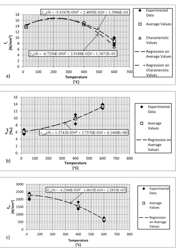
4.5 Mortar

4.5.1 Mortar type M5

The mortar M5 showed small increases of strength up to 400°C and a high level

of reduction with a maximum of 50% for higher temperatures (Figure 4.8a). As

for the block materials, increments of ultimate strain of about 100% were

recorded, respect to the values estimated with the TEST 1 – CMC (Figure 4.8b).

Correspondingly, the apparent modulus of elasticity shows a significant reduction

up to one third for 600°C, respect to the results from TEST 1 – CMC (Figure

4.8c).

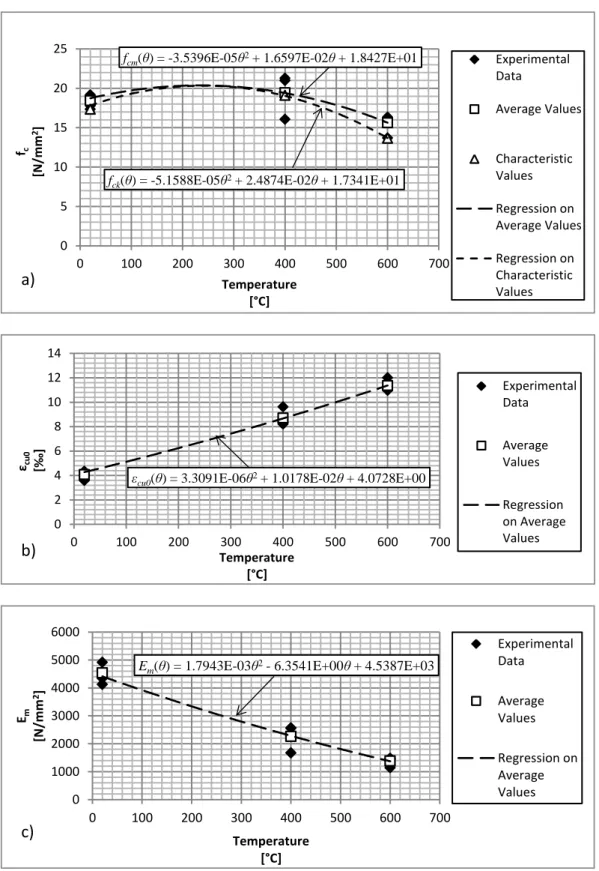
4.5.2 Mortar type M10

Samples of mortar M10 showed smaller reductions of the compressive strength at

600°C (Figure 4.9a), while in terms of ultimate strain they showed increases

comparable to those of mortar M5 (Figure 4.9b). The apparent modulus of

elasticity presents an almost linear decreasing of about 5.39 °C-1N/mm2 (Figure

fcm(θ) = -5.4347E-05θ2+ 2.4095E-02θ + 1.3986E+01

fck(θ) = -6.7256E-05θ2+ 2.9188E-02θ + 1.3671E+01

0 2 4 6 8 10 12 14 16 18 0 100 200 300 400 500 600 700 fc [N /m m 2] Temperature [°C] Experimental Data Average Values Characteristic Values Regression on Average Values Regression on Characteristic Values

εcu0(θ) = 1.3741E-05θ2+ 3.7576E-03θ + 6.1468E+00

0 2 4 6 8 10 12 14 16 0 100 200 300 400 500 600 700 800 εcu0 [‰] Temperature [°C] Experimental Data Average Values Regression on Average Values

Em(θ) = -4.2360E-03θ2- 1.6015E-01θ + 2.2853E+03

0 500 1000 1500 2000 2500 3000 0 100 200 300 400 500 600 700 800 Em [N /m m 2] Temperature [°C] Experimental Data Average Values Regression on Average Values

Fig. 4.8: Mortar M5: a) Compressive strength (fc). b) Ultimate strain (εcu0). c) Young Modulus of Elasticity

(Em). a)

b)

f_cm(θ) = -3.5396E-05θ2_{+ 1.6597E-02θ + 1.8427E+01}

fck(θ) = -5.1588E-05θ2+ 2.4874E-02θ + 1.7341E+01

0 5 10 15 20 25 0 100 200 300 400 500 600 700 fc [N /m m 2] Temperature [°C] Experimental Data Average Values Characteristic Values Regression on Average Values Regression on Characteristic Values

εcu0(θ) = 3.3091E-06θ2+ 1.0178E-02θ + 4.0728E+00

0 2 4 6 8 10 12 14 0 100 200 300 400 500 600 700 εcu0 [‰] Temperature [°C] Experimental Data Average Values Regression on Average Values

Em(θ) = 1.7943E-03θ2- 6.3541E+00θ + 4.5387E+03

0 1000 2000 3000 4000 5000 6000 0 100 200 300 400 500 600 700 Em [N /m m 2] Temperature [°C] Experimental Data Average Values Regression on Average Values

Fig. 4.9: Mortar M10: a) Compressive strength (fc). b) Ultimate strain (εcu0). c) Young Modulus of Elasticity

(Em). a)

b)

4.6 Reduction factors definition

As for reinforced concrete and constructional steel in EN 1992-1-2 [48] and EN

1993-1-2 [49], the reduction factors can be defined dividing the expression (4.1)

for the coefficient A0, that is

 

where kX represents the ratio between the value of the generic mechanical property

at the temperature θ and that at room temperature. The values of the coefficients

A1/A0 and A2/A0 in the relation (4.3) for fcm, fck, εcu0 and E for each tested material

are indicated in the Tables 4.4 and 4.5, and the graphs of the functions are shown

in the Figures 4.10, 4.11, 4.12 and 4.13. It’s easy to observe as the kX coefficients

of CLAY remain close to the unit value: it confirms that this material is one of the

least sensitive to high temperatures and one of the most efficient when exposed to

fire. Furthermore, although all the materials present increments of ultimate strain

with the temperature rise with a consequent reduction of the modulus of elasticity,

only the mortars and the AAC show appreciable increases of compressive strength

Mechanical

Property A1/A0 A2/A0

CLAY

fcm -2.13E-05 0.00E+00

fck -2.96E-04 0.00E+00

εcu0 3.61E-04 0.00E+00

Eb -2.72E-04 0.00E+00

AAC

fcm 9.34E-04 -1.67E-06

fck 7.13E-04 -1.42E-06

εcu0 1.12E-03 0.00E+00

αth -3.22E-03 2.23E-06

Eb -3.04E-04 -6.69E-07

LWC

fcm 9.65E-05 -1.08E-06

fck 2.16E-04 -1.11E-06

εcu0 6.02E-04 2.08E-06

Eb -1.14E-03 0.00E+00

LWC-LAP

fcm -5.58E-04 0.00E+00

fck -6.91E-04 0.00E+00

εcu0 2.27E-03 -1.19E-06

Eb -1.19E-03 0.00E+00

LWC-FV

fcm -2.34E-04 0.00E+00

fck -8.79E-05 0.00E+00

εcu0 1.23E-03 4.60E-07

Eb -9.64E-04 0.00E+00

Mechanical

Property A1/A0 A2/A0

Mortar M5

fcm 1.72E-03 -3.89E-06

fck 2.14E-03 -4.92E-06

εcu0 6.11E-04 2.24E-06

Em -7.01E-05 -1.85E-06

Mortar M10

fcm 9.01E-04 -1.92E-06

fck 1.43E-03 -2.97E-06

εcu0 2.50E-03 8.12E-07

Em -1.40E-03 3.95E-07

Tab. 4.5: Ratios Ai/A0 of equation (4.3) for tested mortars.

0.00E+00 2.00E-01 4.00E-01 6.00E-01 8.00E-01 1.00E+00 1.20E+00 1.40E+00 0 100 200 300 400 500 600 700 kfc m (θ ) Temperature [°C] CLAY AAC LWC LWC-LAP LWC-FV Mortar M5 Mortar M10

0.00E+00 2.00E-01 4.00E-01 6.00E-01 8.00E-01 1.00E+00 1.20E+00 1.40E+00 0 100 200 300 400 500 600 700 kfck (θ ) Temperature [°C] CLAY AAC LWC LWC-LAP LWC-FV Mortar M5 Mortar M10

Fig. 4.11: Reduction factor kfck in function of temperature θ.

0.00E+00 5.00E-01 1.00E+00 1.50E+00 2.00E+00 2.50E+00 3.00E+00 3.50E+00 0 100 200 300 400 500 600 700 kεc u0 (θ ) Temperature [°C] CLAY AAC LWC LWC-LAP LWC-FV Mortar M5 Mortar M10

0.00E+00 2.00E-01 4.00E-01 6.00E-01 8.00E-01 1.00E+00 1.20E+00 0 100 200 300 400 500 600 700 kE (θ ) Temperature [°C] CLAY AAC LWC LWC-LAP LWC-FV Mortar M5 Mortar M10

Fig. 4.13: Reduction factor kE in function of temperature θ.

4.7 Prediction of the masonry modulus of elasticity: an

application of the “Pile Model”

A simple way to simulate the mechanical behavior in the elastic field of a

masonry panel is the well-known elastic layered model proposed by Hilsdorff

[50]. This approach, in the particular case of simple load of uniform compression,

is identifiable as the Pile Model [51, 52]. Referring to Figure 4.14, and treating the

problem in the x-z plane, the equilibrium in the horizontal direction x of the

average values of normal stresses x in thickness hands

xm ms xb bs

  , (4.4)

in which the quantities refer to mortar (m) and blocks (b). The corresponding

congruence strain in the same direction on the average in thickness, assuming that

xm xb

  , (4.5)

The elastic constitutive law for mortar and blocks provides the equations









where b and m are respectively the Poisson moduli of each material component,

while z is the uniform vertical normal stress (the same for mortar and block

layers). Rearranging the equations of equilibrium, congruence and elasticity, it

can be obtain: xm z xb z r         , (4.7)

where the dimensionless coefficients r, n and  are

b m b m s r s E n E   , (4.8)









The apparent Young modulus E of masonry panel along vertical direction z is

given by









If the Young moduli of mortar Em and blocks Eb are depending from temperature,

equation (4.10) becomes:

 

_{   }

For example, we report the curves for the CLAY blocks masonry with mortar M5

modulus E of the panel as a function of temperature  and parameterized respect to the factor r.

The tests at various temperatures even showed that Eb is greater than Em. If we

assume the equality of Poisson moduli, being evidently r > 1, expressions (4.7)

show that mortar is compressed while the blocks are transversely in tension; the

first contribution is related to the bearing capacity as it corresponds to a reduction

in the deviatoric stress tensor in mortar, the second is negative but negligible in

most practical cases, due to the small amount of the factor (1/r). Moreover, at high

temperatures, the cohesion between blocks and mortar could be modified. The

following expression by EN 1996-1-1 [23]:

k b m

f K f f, (4.12)

could be calibrated in terms of  and , taking into account that in cold condition are 0.7 0.3     . (4.13)

Then we could estimate the characteristic compressive strength fk of masonry

panels, from the proposed experimental curves, for the different materials and at

various temperatures. This last is a possible perspective for further experimental

0 200 400 600 800 1000 1200 1400 0 100 200 300 400 500 600 700 800 E( θ,r ) [N/m m 2] Temperature [°C] r = 5 r = 10 r = 15 r = 20 0 200 400 600 800 1000 1200 1400 0 100 200 300 400 500 600 700 800 E( θ, r) [N/m m 2] Temperature [°C] r = 5 r = 10 r = 15 r = 20

a)

b)

Fig. 4.15: Calculated apparent Young Modulus of Elasticity for masonry – a) CLAY units and Mortar M5. b)

CLAY units and Mortar M10.

4.8 Uniaxial constitutive law determination

4.8.1 The Popovič model

It was chosen to consider the following Popovič model for properties and the guarantees offered in the post-critical behaviour, as described in [53]. As in EN

1992-1-2 [48] for concrete, this model was adapted to the variation of the

mechanical properties with high temperatures, assuming the following form:





 

_{ }

 

where the n parameter characterizes each type of material, regardless of the

temperature (Figure 4.16). An important property of the function (4.14) regards its

shape when n assumes high values. Indeed, as n tends to +∞, the Popovič model

tends to the first sawtooth form for non negative values of the strain.

Instead as n tends to 1, the model assumes the rigid – plastic constitutive law.

The determination of the parameter n was carried out considering the full pairs of

dimensionless values (σ/fc(θ); ε/εcu0(θ)) (both belonging to the range [0; 1])

recorded during the execution of the tests on each specimen. In this way the

expression (4.14) can assume the following form:

 

where s and e are respectively the ratios σ/fc(θ) and ε/εcu0(θ).

The value of n that minimizes the mean squared error has been determined by

applying the non-linear regression algorithm of Levenberg–Marquardt, based on

n   0  cu      ˆ ,     c f 0 0.1 0.2 0.3 0.4 0.5 0.6 0.7 0.8 0.9 1 0 0.2 0.4 0.6 0.8 1 σ (ε ,θ )/ fc (θ ) ε/εcu0(θ) n = 1.00 n = 1.05 n = 1.20 n = 1.50 n = 3.00 n = 10.00 n →+∞ a) b)

Fig. 4.16: Popovič model: a) 3D graph. b) Dimensionless stress-strain parametric curves.

4.8.2 Application of Levenberg–Marquardt Algorithm

As in its primary application, the Levenberg–Marquardt algorithm is used for the

independent and dependent variables (ei, si) and the optimization problem

concerns the determination of the parameter n so that the sum of squares of the

deviation S(n) defined as

 







The Levenberg–Marquardt algorithm provides an iterative procedure, at the

beginning of which an initial guess value for the parameter n0 must be given. In

each iteration step, the parameter value n, is replaced by a new estimate, n + δ. To

determine δ, the functions ŝ(ei, n + δ) are approximated by their linearization:



 







At the minimum of the sum of squares S(n), its derivative with respect to δ tends

to 0. Substituting in (4.16) the first order approximation (4.17), we obtain:



















 

 

with obvious meaning of the symbols s, ŝ and e.

In this case, the Jacobian matrix J assumes the form of the gradient vector:

 

  n

so that the expression (4.19) can be placed in the form:





 

Taking the derivative of (4.21) with respect to δ and placing the results to 0, we

have:

 

 





_

_









The equation (4.23) is placed in the following damped version for optimizing the

calculus and convergence procedure:

 









_

_













where non negative damping factor λ is adjusted at each iteration.

The Levenberg–Marquardt procedure was applied to the whole sets of readings

recorded during the experimental campaign execution. The total number of these

pairs of values for each material had an order of 104÷105 and is reported in Table

4.6.

The n parameters with the functions (4.15) obtained for each material are shown

in Figure 4.17, where a high value for CLAY is calculated. According to the

parametric curves provided by EN 1996-1-2 [1] and observing that relevant

differences between shapes and values are not detected, it was chosen to merge

whole data of LWC materials and Mortars respectively in only two sets,

proposing only two values of n for these types. The obtained results and the

related curves are shown in the Figure 4.18 and reported in Table 4.6.

Material Number of pairs of

stress-strain readings n CLAY 161504 115.5 AAC 39911 7.9 LWC 29080 8.2 9.1(*) LWC-LAP 27292 10.8 LWC-FV 17613 9.1 M5 13119 3.4 4.4(*) M10 12786 5.6

Tab. 4.6: Numbers of stress-strain readings and parameter n for each material. (*) results obtained after data

0 0.1 0.2 0.3 0.4 0.5 0.6 0.7 0.8 0.9 1 0 0.2 0.4 0.6 0.8 1 σ /fc ε/εcu0 CLAY - n = 115.5 AAC - n = 7.9 LWC - n = 8.2 LWC-LAP - n = 10.8 LWC-FV - n = 9.1 M5 - n = 3.4 M10 - n = 5.6

Fig. 4.17: Stress-strain models for tested materials with n parameter related values.

0 0.1 0.2 0.3 0.4 0.5 0.6 0.7 0.8 0.9 1 0 0.2 0.4 0.6 0.8 1 σ /fc ε/εcu0 CLAY - n = 115.5 AAC - n = 7.9 LWC - n = 9.1 Mortar - n = 4.4

Fig. 4.18: Stress-strain models for tested materials with “n” parameter related values merging the data of

LWC materials and Mortars.

4.8.3 Validation procedure

It is important to point out the independence of n from the temperature. It was

the regressions done. In fact, in this case k represents the number of temperatures

at which the tests were conducted and the k-folds are the number of sets of all

stress-strain readings taken at the same temperature for the various materials.

A single subsample, among the k ones, was used as validation data for the model

testing, while the remaining k−1 subsamples were used as training data. The

cross-validation process was then repeated k times (the folds), and each of the k

subsamples was used exactly once as validation data. Then, the k results from the

folds can be averaged to produce a single estimation. The advantage of this

validation method is that all observations are used for both training and validation,

at the same time, and each observation is used for validation exactly once.

In this specific case, the Levenberg–Marquardt algorithm was reapplied k times

for the determination of the n value on all the stress-strain readings belonging to

the union of the k-1 sets (training data), and then the mean squared error of that

one related to the generic k set was calculated. This kind of iteration is

summarized in the scheme of Figure 4.19.

In this way, the independence of n from the temperature could be proved. Indeed

the average value of this parameter deduced from the training sets is close to that

obtained over the whole sample of the readings, and that the value of the mean

Fig. 4.19: Scheme of k-fold cross validation.

4.8.4 Obtained results 4.8.4.1 Clay

As already mentioned in the paragraph 4.8.2, a high value of n was detected for

CLAY. As n tends to +∞, the expression (4.14) tends to the linear form for

ε/εcu0(θ)  [0; 1], so for CLAY material a linear constitutive model is proposed

according to the Annex D of EN 1996-1-2 [1] as in the following expression:





 

_{ }

The Figures 4.20 and 4.21 show how the model proposed by Eurocode fit better

with increasing temperature, in agreement with the lower values of the error

the strain and the compressive strength is too low compared to the experimental

data; in particular, the ultimate strain values provided by Eurocode belong to the

range 1.8÷ 3.0 ‰, while the experimental curves reach approximately 7.0 ‰.

The mean square percentage error produced by parametric curves of Annex D of

EN 1996-1-2 [1] is 266.6%, while the proposed model can reduce it up to 6 times.

The k-fold cross validation shows that the value of n calculated on each trainset

assumes an average value greater than 100, and the values of the mean squared

error calculated on the average testsets remain stable at about 3×10-3. This

0 50 100 150 200 250 0 100 200 300 400 500 600 700 n

Temperature related to k-th validation subset

n n_ trained n_average 0 0.001 0.002 0.003 0.004 0.005 0.006 0 100 200 300 400 500 600 700 M SE

Temperature related to k-th validation subset

mse mse_validated mse_average a) b) c)

Fig. 4.20: CLAY: a) Comparison between EN 1996-1-2 [1] and proposed model with experimental curves; b)

n parameter values from k-fold cross validation; c) mean squared error (MSE) for each iteration of k-fold

0 10 20 30 40 50 0 1 2 3 4 5 6 7 σ [MP a] ε [‰] θ = 20°C 0 10 20 30 40 50 0 1 2 3 4 5 6 7 σ [MP a] ε [‰] θ = 200°C 0 10 20 30 40 50 0 1 2 3 4 5 6 7 σ [MP a] ε [‰] θ = 500°C 0 10 20 30 40 50 0 1 2 3 4 5 6 7 σ [MP a] ε [‰] θ = 700°C 0 10 20 30 40 50 0 1 2 3 4 5 6 7 σ [MP a] ε [‰] θ = 100°C 0 10 20 30 40 50 0 1 2 3 4 5 6 7 σ [MP a] ε [‰] θ = 400°C 0 10 20 30 40 50 0 1 2 3 4 5 6 7 σ [MP a] ε [‰] θ = 600°C 0 10 20 30 40 50 0 1 2 3 4 5 6 7 σ [MP a] ε [‰] θ = 600°C Experimental Curves EC6-1-2 Aver. EC6-1-2 Char. Proposed Model Aver. Proposed Model Char.

4.8.4.2 AAC

The Figures 4.22 and 4.23 show how the Eurocode model fit well for

temperatures up to 200°C. For higher temperatures, the values of the strain and

compressive stress are much too high compared to the experimental readings; in

particular, the strains provided by Eurocode exceed the threshold of 40‰, while

the experimental curves not even reach that of 7.0 ‰.

The mean square percentage error produced by parametric curves of Annex D of

EN 1996-1-2 [1] is 34.8%, while the proposed model can reduce it to 5.8%.

The cross-validation shows that the value of n calculated on each trainset always

assumes an average value close to 7.9, while the average mean squared error

calculated on the testsets remains stable at about 2.5×10-3÷3.5×10-3, except for

that related to 500°C where evidently the proposed model fails to fit with the same

7.2 7.4 7.6 7.8 8 8.2 0 100 200 300 400 500 600 700 n

Temperature related to k-th validation subset

n n_ trained n_average 0 0.0005 0.001 0.0015 0.002 0.0025 0 100 200 300 400 500 600 700 M SE

Temperature related to k-th validation subset

mse mse_validated mse_average b) c) a)

Fig. 4.22: AAC: a) Comparison between EN 1996-1-2 [1] and proposed model with experimental curves; b)

n parameter values from k-fold cross validation; c) mean squared error (MSE) for each iteration of k-fold

0 1 2 3 4 5 6 7 0 10 20 30 40 50 σ [MP a] ε [‰] θ = 20°C 0 1 2 3 4 5 6 7 0 10 20 30 40 50 σ [MP a] ε [‰] θ = 100°C 0 1 2 3 4 5 6 7 0 10 20 30 40 50 σ [MP a] ε [‰] θ = 200°C 0 1 2 3 4 5 6 7 0 10 20 30 40 50 σ [MP a] ε [‰] θ = 400°C 0 1 2 3 4 5 6 7 0 10 20 30 40 50 σ [MP a] ε [‰] θ = 500°C 0 1 2 3 4 5 6 7 0 10 20 30 40 50 σ [MP a] ε [‰] θ = 600°C 0 1 2 3 4 5 6 7 0 10 20 30 40 50 σ [MP a] ε [‰] θ = 700°C 0 10 20 30 40 50 0 1 2 3 4 5 6 7 σ [MP a] ε [‰] θ = 600°C Experimental Curves EC6-1-2 Aver. EC6-1-2 Char. Proposed Model Aver. Proposed Model Char.

4.8.4.3 Lightweight aggregate concrete

The Eurocode model fits better at room temperature but gives incorrect values for

all three types of lightweight aggregate concrete from 400°C to 600°C, as shown

in Figures 4.24, 4.25, 4.26, 4.27, 4.28 and 4.29. The proposed model for LWC

produces a mean squared percentage error on all the readings equal to 47.9%,

while the respective group of parametric curves provided by Eurocode gives

107.7%. As shown in Figure 4.24, the error obtained with the k-fold cross

validation on all testset is about 2.5×10-3, with the exception of that one

corresponding to 500°C, where it is reduced to 1.4×10-3. The proposed value of n

and the averaged one over the trainsets are close, so it confirms the validity of the

model on each testset.

The proposed model for LWC-LAP produces a mean squared percentage error

equals to 13.2% versus 65.6% relative to the model of Eurocode. The error

determined with the cross validation is lower on testsets related to higher

temperatures. The n validated on testsets to 400 ° C and 600 ° C are higher than

the average and the proposed one.

The mean squared percentage error of the LWC-FV model is lower than the other

two lightweight aggregate concretes tested and is equal to 10.2% against 69.7%

produced by Eurocode curves. This is probably due to the smaller number of

available experimental data. The n validated on testsets at room temperature and

600°C are different than the average and proposed one that, however, are very

close together. Consequently, the errors at the extremes of the range of tested

0 2 4 6 8 10 12 0 100 200 300 400 500 600 700 n

Temperature related to k-th validation subset

n n_ trained n_average 0 0.0005 0.001 0.0015 0.002 0.0025 0.003 0.0035 0.004 0 100 200 300 400 500 600 700 M SE

Temperature related to k-th validation subset

mse mse_validated mse_average a) b) c)

Fig. 4.24: LWC: a) Comparison between EN 1996-1-2 [1] and proposed model with experimental curves; b)

n parameter values from k-fold cross validation; c) mean squared error (MSE) for each iteration of k-fold

0 2 4 6 8 10 12 14 0 100 200 300 400 500 600 700 n

Temperature related to k-th validation subset

n n_ trained n_average 0 0.0005 0.001 0.0015 0.002 0.0025 0.003 0.0035 0 100 200 300 400 500 600 700 M SE

Temperature related to k-th validation subset

mse mse_validated mse_average a) b) c)

Fig. 4.25: LWC-LAP: a) Comparison between EN 1996-1-2 [1] and proposed model with experimental

curves; b) n parameter values from k-fold cross validation; c) mean squared error (MSE) for each iteration of

0 2 4 6 8 10 12 14 16 18 0 100 200 300 400 500 600 700 n

Temperature related to k-th validation subset

n n_ trained n_average 0 0.002 0.004 0.006 0.008 0.01 0.012 0 100 200 300 400 500 600 700 M SE

Temperature related to k-th validation subset

mse mse_validated mse_average a) b) c)

Fig. 4.26: LWC-FV: a) Comparison between EN 1996-1-2 [1] and proposed model with experimental curves;

b) n parameter values from k-fold cross validation; c) mean squared error (MSE) for each iteration of k-fold cross validation.

0 5 10 15 20 25 0 10 20 30 40 50 σ [MP a] ε [‰] θ = 20°C 0 5 10 15 20 25 0 10 20 30 40 50 σ [MP a] ε [‰] θ = 400°C 0 5 10 15 20 25 0 10 20 30 40 50 σ [MP a] ε [‰] θ = 500°C 0 5 10 15 20 25 0 10 20 30 40 50 σ [MP a] ε [‰] θ = 600°C 0 5 10 15 20 25 0 10 20 30 40 50 σ [MP a] ε [‰] θ = 600°C

Experimental Curves EC6-1-2 Aver. EC6-1-2 Char. Proposed Model Aver. Proposed Model Char.

Fig. 4.27: LWC: Comparison between EN 1996-1-2 [1] and proposed model with experimental curves.

0 5 10 15 20 25 0 10 20 30 40 50 σ [MP a] ε [‰] θ = 20°C 0 5 10 15 20 25 0 10 20 30 40 50 σ [MP a] ε [‰] θ = 400°C 0 5 10 15 20 25 0 10 20 30 40 50 σ [MP a] ε [‰] θ = 600°C 0 10 20 30 40 50 0 1 2 3 4 5 6 7 σ [MP a] ε [‰] θ = 600°C Experimental Curves EC6-1-2 Aver. EC6-1-2 Char.

Proposed Model Aver.

Proposed Model Char.

0 10 20 30 40 50 0 1 2 3 4 5 6 7 σ [MP a] ε [‰] θ = 600°C Experimental Curves EC6-1-2 Aver. EC6-1-2 Char. Proposed Model Aver. Proposed Model Char. 0 5 10 15 20 25 30 35 0 10 20 30 40 50 σ [MP a] ε [‰] θ = 20°C 0 5 10 15 20 25 30 35 0 10 20 30 40 50 σ [MP a] ε [‰] θ = 400°C 0 5 10 15 20 25 30 35 0 10 20 30 40 50 σ [MP a] ε [‰] θ = 600°C

Fig. 4.29:. LWC-FV: Comparison between EN 1996-1-2 [1] and proposed model with experimental curves.

4.8.4.4 Mortar

The models proposed for mortar M5 and M10 (Figures 4.30, 4.31, 4.32 and 4.33)

produce mean squared percentage errors respectively of 5.6% and 6.9%. For the

mortar M5, the value of n validated on the testset related to 400°C is lower than

the proposed one and, at this temperature, the maximum value of the errors is

detected with the k-fold cross validation. For the mortar M10, instead, the value of

n validated at 400°C and 600°C is higher than proposed one, and the maximum value of the errors is obtained at room temperature.

0 2 4 6 8 10 12 14 16 0 100 200 300 400 500 600 700 0 2 4 6 8 10 12 14 16 18 Strain [‰] Temperature [°C] S tr e s s [ M P a ] 0 2 4 6 8 10 12 14 16 Experimental Curves Proposed Model 0 0.5 1 1.5 2 2.5 3 3.5 4 4.5 5 0 100 200 300 400 500 600 700 n

Temperature related to k-th validation subset

n n_ trained n_average 0 0.002 0.004 0.006 0.008 0.01 0 100 200 300 400 500 600 700 M SE

Temperature related to k-th validation subset

mse mse_validated mse_average a) b) c)

Fig. 4.30: Mortar M5: a) Comparison between EN 1996-1-2 [1] and proposed model with experimental

curves; b) n parameter values from k-fold cross validation; c) mean squared error (MSE) for each iteration of

0 2 4 6 8 10 12 14 0 100 200 300 400 500 600 700 0 5 10 15 20 25 Strain [‰] Temperature [°C] S tr e s s [ M P a ] 0 2 4 6 8 10 12 14 16 18 20 Proposed Model Experimental Curves 0 1 2 3 4 5 6 7 0 100 200 300 400 500 600 700 n

Temperature related to k-th validation subset

n n_ trained n_average 0 0.001 0.002 0.003 0.004 0.005 0 100 200 300 400 500 600 700 M SE

Temperature related to k-th validation subset

mse mse_validated mse_average a) b) c)

Fig. 4.31: Mortar M10: a) Comparison between EN 1996-1-2 [1] and proposed model with experimental

curves; b) n parameter values from k-fold cross validation; c) mean squared error (MSE) for each iteration of

0 10 20 30 40 50 0 1 2 3 4 5 6 7 σ [MP a] ε [‰] θ = 600°C Experimental Curves EC6-1-2 Aver. EC6-1-2 Char.

Proposed Model Aver.

Proposed Model Char. 0 5 10 15 20 0 5 10 15 20 σ [MP a] ε [‰] θ = 20°C 0 5 10 15 20 0 5 10 15 20 σ [MP a] ε [‰] θ = 400°C 0 5 10 15 20 0 5 10 15 20 σ [MP a] ε [‰] θ = 600°C

Fig. 4.32: Mortar M5: Comparison between EN 1996-1-2 [1] and proposed model with experimental curves.

0 10 20 30 40 50 0 1 2 3 4 5 6 7 σ [MP a] ε [‰] θ = 600°C Experimental Curves EC6-1-2 Aver. EC6-1-2 Char.

Proposed Model Aver.

Proposed Model Char. 0 5 10 15 20 25 0 5 10 15 20 σ [MP a] ε [‰] θ = 20°C 0 5 10 15 20 25 0 5 10 15 20 σ [MP a] ε [‰] θ = 400°C 0 5 10 15 20 25 0 5 10 15 20 σ [MP a] ε [‰] θ = 600°C