14
3 Trajectory Optimization problem
3.1 Introduction
Trajectory optimization is a field of Optimal Control that has a great variety of applications. It involves finding which controls yield the “optimal trajectory” for the specific problem. The definition of what an “optimal” trajectory is changes from problem to problem: in many problems optimality coincides with quickness, i.e. the optimal trajectory is the one that takes the minimum time to reach the final conditions. However other definitions of optimality may involve completely different factors, like fuel consumption or comfort.
3.2 Definition of the problem
Let’s call t the independent variable of the problem:
t0≤ t≤ tf Eq. 3.1
Usually t is the time, as the name suggests, and this thesis will refer to this case; however this may not always be the best choice from the analytical point of view. The dynamic of the problem is described by a set of dynamic variables q, which contains the vectors x and u, respectively the state vector and the control vector, and the time-independent parameters ρ:
ρ
) ( ) ( t u t x = q Eq. 3.2The system dynamic is described by a set of differential equations called the state equations:
[
x(t),u(t),ρ,t]
f=
x& Eq. 3.3
Trajectory optimization problems usually involve other conditions on the variables q during trajectory. These can be initial and final conditions in the form:
[
]
[
f f f]
fu f fl g x(t ),u(t ),ρ,t q q q t ρ, ), u(t ), x(t g q ≤ ≤ ≤ ≤ 0 0 0 0 0u 0l Eq. 3.415
[
]
ul h x(t),u(t),ρ,t h
h ≤ ≤ Eq. 3.5
Both forms are intentionally generic to take account for the most various conditions on the variables. Constraints in eq. 3.4 are known as boundary constraints, while eq. 3.5 represents the path constraints.
Note that path constraints can also be written as:
[
x(t),u(t),ρ,t]
≤0h Eq. 3.6
with an easy manipulation.
The trajectory optimization problem can now be defined, for the system and the constraints defined above, as finding the trajectory which minimizes the performance index:
[
]
[
]
dt t ρ t, u(t), x(t), L + ρ , t ), x(t , t ), x(t = J f t f f∫
0 0 0 ϕ Eq. 3.7along with the optimal control u(t), the parameters ρ and the initial and final conditions of the dynamic system. The first addendum of eq. 3.7 is called the Mayer term of the index, while the integral is the Lagrange term.
Some complex trajectory problems may involve discontinuities in both the dynamic variables and the laws of motion; for example optimizing the trajectory of a multistage rocket launch would require for the mass to change discontinuously, and for the equation of motion to change accordingly. Problem of this kind involve the use of phases (see [3] and [20]), linked by the so-called event constraints. During this thesis no phases were needed.
3.3 Optimal Control Theory
The field of knowledge referred as Optimal Control Theory (OCT) is an extension of Calculus of Variation that deals with the problem of finding the control history that optimizes a given performance index. OCT has applications in both continuous and discrete systems. This paragraph of the thesis is intended to giveonly a brief introduction to OCT; the reader will find in ref. [4] and [19] an exhaustive explanation of the theory.
For the sake of simplicity, assume that initial conditions for the states x(t0) are given, that final time tf and parameters ρ are fixed, and that there are no equality nor inequality constraints. With respect to the notation used in eq. 3.7, the Hamiltonian of the problem is defined as:
16
( )
[
x(t),u(t), t t]
= L[
x(t),u(t),t]
+λ (t)f[
x(t),u(t),t]
H
λ
, T Eq. 3.8where the unknown vectors λ(t) are the vectors of the Lagrange multipliers (LM), relative to the state equations. LM are also known under the term co-states. The LM are an essential and powerful tool of OCT; they allow for the constraints of the problem to be included directly into the equations. Also, they are useful to understand the behaviour of the solution with respect to the constraints.
With eq. 3.8 in mind, OTC states that a necessary condition for u to be the optimal control is to satisfy the following system of differential equations:
∂ ∂ − ∂ ∂ − ∂ ∂ − ≤ ≤ ∂ ∂ t) u, f(x, = x x f λ x L = x H = λ t t t ; = u H T T f & & 0 0 Eq. 3.9
with the boundary conditions assigned:
T f f ) x(t = ) λ(t x = ) x(t ∂ ∂
ϕ
0 0 Eq. 3.10This set of differential equations and boundary conditions is known as the Euler-Lagrange equations; note that since the equations are coupled obtaining a solution can be difficult even for simple problems.
This version of the Euler-Lagrange equations is not universal, because of the assumptions that have been made at the start of this paragraph. Different starting assumptions lead for other terms to be included in order to accommodate boundary and path constraints, but the formulation stays basically the same.
The sufficient condition also assumes various formulations if the problem presents fixed or free final time, constraints on the final or initial conditions, etc. Providing various ad hoc versions of the sufficient condition is not in the intentions of the author; let’s just say that sufficient conditions formulations derive from the simple assumption that:
17 f t t t , u(t) J(t) ≤ ≤ > ∂ ∂ 0 2 2 0 Eq. 3.11
that is, that the Hessian of the performance index with respect to the control is definite positive during the entire trajectory.
3.4 Indirect methods
Indirect methods solve the TO problem without directly solving the Euler-Lagrange differential equation system. The following paragraphs present two methods, both of the Indirect Shooting methods family: Indirect Shooting and Indirect Multiple-Shooting methods.
3.4.1 Indirect Shooting Method
This method tries to find an optimal solution in an iterative way. As already seen, most optimization problems have some of initial and final states and LM values fixed or constrained. Indicating with λ the vector of the LM, this can be formulated as:
[
p(t0 ),t0,p(t ),t]
=0 x p f f φ λ = Eq. 3.12If the set p0 at time t0 is guessed, it becomes possible to solve the Euler-Lagrange system by simple integration in time. The resulting control is obviously sub-optimal since we only guessed the initial condition of p. The sub-optimal control yields a value of φ~, which will also be sub-optimal and will be different from zero. The principle behind this method is that the error ∆
φ
is an index of how wrong our first guess was, and that it can be used to adjust the “aim” of the previous guess: the initial guess p(t0) is adjusted accordingly to the error, moving toward the boundary satisfaction φ~−φ =0.One method to do so is with the transition matrix. The transition matrix is the square matrix )
p(t ) p(tf /∂ 0
∂ , i.e. the matrix of the first derivates of p(tf) with respect to p(t0). Inverting the transition matrix it’s possible to get Δp(t0) such that:
0 0 0 ∆p(t )= ) p(t ) p(t ) ∆p(t f T f ∂ ∂ − Eq. 3.13
with Δp(tf) the error in the final states and co-states. This is similar in nature to the simple Newton’s method: however obtaining the transition matrix can be very difficult.
18
Another procedure is the Backward-sweep algorithm. Instead of guessing p(t0) to obtain p(tf), p(tf) is guessed straight away and integrated backward to get p(t0). Now choose a perturbation δp(t0) of the initial conditions that come closer to the desired p(t0): integrating the Euler-Lagrange equations with p(t0) = δp(t0) yields the perturbation in the final conditions δp(tf). Next step is to sum δp(tf) to the previous guess of p(tf) and to use that as a new guess for the algorithm until convergence. With this method it’s necessary to repeatedly integrate the Euler-Lagrange equations, but the construction of the transition matrix is circumvented.
Summarising, the Indirect Shooting method, as its name suggests, tries to find the optimal solution of the first order optimality conditions, starting from a guess and then correcting the “aim”. Both methods aren’t very easy, since one requires the transition matrix, and the other requires multiple integration of the Euler-Lagrange equations. However, the most subtle issue of the method is that, even for small error in the first guess, we could get very large errors in the boundaries, especially if the time-to-go tf isn’t small. In fact, the error could exceed the numerical range of the computer (see [4], pag. 214).
This sensibility can be reduced by imbedding the problem, i.e. solving a sequence of simpler problems that converge to the first one and using the solution of the previous problem as a guess for the next [3].
3.4.2 Indirect Multiple-Shooting method
This method was developed to reduce the problem of sensibility illustrated in the above paragraph. Imagine dividing the time interval into N smaller intervals:
[
t ,t , ,tN ,tN =tf]
=
t 0 1 ... −1 Eq. 3.14
In this method the values of states and LM at each mesh point ti are also guessed, in addition to the vector p(t0), thus transforming the TO problem in N Initial Value problems (see [3], par. V). However, since we want both state and LM to be continuous, additional linkage constraints must be satisfied, in the form:
0 = ) p(t ) p(t = ψi i− − i+ Eq. 3.15
With this method the sensibility of the algorithm is reduced since the propagation of the error in the Hamiltonian derivatives is limited to a small amount of time.
As in the Indirect Shooting method, at each iteration the previous guess is renewed in order to find the root of both eq. 3.12 and eq. 3.15, i.e. to satisfy both boundary and linkage constraints.
19
The Indirect Multiple-Shooting method is very successful in its main goal, which is increasing robustness of the algorithm. However, this is done by greatly increasing the number of variables and constraints for the problem. In addition, guessing values for the intermediate state and co-states may not be an immediate choice.
Another trait of the Indirect Multiple-Shooting method is that, since no requests are made on the continuity of the control vector, this can result in it to be discontinuous. This is not necessarily an issue since it may be used to better represent optimal control solutions that are discontinuous on their own.
The Indirect Multiple-Shooting method is then an overall improvement over the Indirect
Shooting method, except for those simple problems for which the increased complexity of the multiple-shooting approach is not required.
3.4.3 Overview of Indirect methods
Probably the worst flaw of these methods is that a lot of difficult derivatives must be computed for solving the Euler-Lagrange equations and this leads to inefficiency in the solving.
It also needs to be noted that in numerous fields of interest, lookup tables are commonly used instead of analytical functions; the most common use of such lookup tables is for linear interpolation, which makes data representation not differentiable in table points.
The indirect methods as a whole have been substituted in more recent applications by newer methods, i.e. the direct methods.
3.5 Direct methods
3.5.1 Non-Linear Programming
In order to explain the direct methods appropriately, the non-linear programming (NLP) problem must be introduced. This problem consists in finding the n scalar values qi that minimize:
ℜ → ℜ ∈ n n q q n F(q ,q , q ) f : .... min 1 2 ... 1 Eq. 3.16
20 0 ... 0 ... 2 1 2 1 ≤ ) q , q , (q c = ) q , q , (q c n I n E Eq. 3.17
If a constraint is satisfied with the equal sign, then it belongs to the so-called active set. Note that the above formulas can be interpreted both as scalar and vector, i.e. cE and cI can be vectors or scalars. Define now the parameters’ set p and the Hamiltonian H as:
(
q ,q qn)
p≡ 1 2…[
]
=F(p)+λ c(p) p c p c λ λ + F(p) λ) H(p, T I E T I T E ≡ ) ( ) ( Eq. 3.18where λ is the vector of the LM. The vector p essentially represents a point in the n-dimension space of parameters qi in which F is defined. Define also:
The vector p is said to be a regular point if the constraints belonging to the active set cas are linearly independent. Note that for a regular point the number of constraints in the active set cannot be greater then the number of the parameters, otherwise the problem has no solution. Now, for a point p* to be a local minimum for F, it must exist λ* such that:
0 *,λ )= F(p )+λ C (p )+λ C (p )= H(p p ET E IT I p ∗ ∇ ∗ ∗ ∗ ∇ 0 = ) (p CE ∗ 0 ≤ ∗ ) (p CI 0 *≥ I λ
( )
* 0 * , ,icEi p = Eλ
Eq. 3.20Another necessary condition on p* is that: 0 2 2 ≥ ∂ ∂ d p H dT Eq. 3.21
for every feasible search direction d, i.e. for every direction that does not violate the constraints. Equations 3.20 are known as Kuhn-Tucker conditions.
Now that the NLP problem has been introduced, consider again the Trajectory Optimization (TO) problems. A TO problem can be defined as:
p c (p) C E E ∂ ∂ ≡ p c (p) C I I ∂ ∂ ≡
( )
p F p F(p) (p) gT =∇p ∂ ∂ ≡ Eq. 3.1921
[
]
[
]
dt t ρ t, u(t), x(t), L + ρ , t ), x(t , t ), x(t f t f f t q∫
0 0 0 ) ( min ϕ[
x(t),u(t),ρ,t]
=0 f x −&[
q(t),t,ρ]
=0 cE[
q(t),t,ρ]
≤0 cI ρ
u x = q f t t t0 ≤ ≤ Eq. 3.22with x and u being state and control vector, ρ being the parameters of the problem, and vectors cE and cI representing the constraints. Optimal Control theory gives the analytical solution of the problem. However such solution can be very hard to obtain even for relatively simple problems. Instead, direct methods transpose optimal control problems into much easier NLP problems. There are 3 direct methods currently available for solving Optimal Control problems. The first two methods are the Direct Shooting and the Direct Multiple-Shooting method, of the family of the Shooting methods. Direct Shooting methods solve the NLP problem using only the control as a parameter, and compute the state accordingly to the initial conditions and the dynamic constraints.
The last method, the Direct Collocation method, uses both control and states as parameters for the optimization, paying attention not to violate the dynamic constraints at the same time. As a consequence of this choice, the dimension of p, i.e. the number of optimization parameters increases, but state values are always under control of the solver and thus won’t diverge.
3.5.2 Direct Shooting and Direct Multiple-Shooting methods
The direct shooting method works as follows. The control parameters are written as linear combination of U sub-functions βi(t) of our choice:
∑
U ⋅ = i i i β(t) c = u(t) 1 Eq. 3.23with ci unknown scalars. The βi(t) sub-functions are often polynomials but there is no restriction on what kind of functions to use.
22
[
]
[
]
[
]
[
]
[
]
0 0 ~ , , , , , , , , , , , n i m 1 0 1 0 1 0 1 0 1 0 0 ≤ − t ρ, , c c , x , x c = t ρ, , c c , x , x c = t c c x x cE t c c x x f x c c ρ, , x , x J c , , x , x N f I N f E N f N f N f i f L L K K & L ρ ρ ρ Eq. 3.24Now, the scalars ci and the components of the vectors ρ, x0 and xf are used as the NLP optimization parameters: the problem is solved as a NLP by changing the set of parameters p until optimality has been reached. As in the Indirect Shooting method, initial starting point p may be far from optimality, and iteration is required to get a good “aim” of the control history.
The method is easy to implement and understand and has a low number of parameters to optimize. On the other hand, it comes with a great sensibility on the parameters, as errors in the guess increase with integration in time (similarly to the Indirect Shooting method).
Another issue of the method is that its efficiency strongly depends on which sub-functions βi(t) are used. A poor choice of the sub-function set can result in suboptimal or even completely wrong solutions [20].
It would seem a good idea to make use of a lot of different sub-functions to have many possible u(t) covered by eq. 3.23. However, it has been observed that the most successful applications of the Direct Shooting method make use of as few sub-functions as possible, thus reducing the computational difficulties, and reducing the error growth with time.
In order to reduce the method’s sensibility a Direct Multiple-Shooting method has been developed. With this method, the time interval is divided in N smaller intervals and in each interval, the control vector is written as:
N , = k (t) β c = (t) u Uk = i k i k i k 1,... 1
∑
⋅ Eq. 3.25In analogy with the Direct Shooting method, cki are unknown scalars and βki(t) are chosen sub-functions. The optimization parameters are now the scalars cki as well as the components of vectors ρ, x0 and xf. However, in addition to constraints of eq. 3.24, the following continuity constraints on the state have to be included in the NLP problem:
23 0 = ) x(t ) x(t = ψi i− − i+ Eq. 3.26
3.5.3 Direct Collocation method
Assuming that the independent variable t, the state vector x and the control vector u of eq. 3.22 are discrete, it’s possible to put the problem in the form:
[
]
[
( ) ( )
i i i]
N = i N N N t ρ, , t u , t x + ρ , t ), x(t , t ), x(t ) q(t t q(0)m…inϕ
0 0∑
1ℓ( )
( )
[
,]
~[
]
0 ) ( ) ( 0 0 0 0 1 = t t ), q(t ) q(t c = t t t q t q c x t x t x N N E N N E i i i … … + − −∆ K K[
0 … N 0… N]
≤0 I q(t ) q(t ),t t c f N =t t < t < t < t0 1 2… Eq. 3.27The term Δxi in second equation of eq. 3.27 can be computed from state and control values. Various algorithms or schemes, such as the Runge-Kutta scheme family, have been developed for this purpose. Schemes are said to be explicit if Δxi is computed only with x(tj), u(ti) and j<i ; otherwise they are called implicit. The difference between the two is that with an explicit method state values can be derived one after another without further elaboration, while with an implicit method the next values of the states and controls need to be guessed, and then the procedure must be reiterated to refine the solution. More information on the subject of schemes can be found in [3].
The discretization of t can be done in multiple ways. A simple way of dealing with it is to use a fixed interval between instants, but non-fixed intervals are also common. Another more complex choice could be using a fixed number of intervals but leaving their length to the optimization tool, as explained later.
With this approach, the TO problem has been transposed as a NLP problem (as can be seen confronting eq. 3.27 with eq. 3.16 and 3.17) in which the optimization parameters are control and states values xi and ui at discrete time instants ti (in addiction to q). This allows for a much more robust computation since the states’ values are always under the direct control of the solver. It also results in more freedom of the solving algorithm, because states value can be changed towards optimality directly instead of needing to be “driven” by the control variables.
The dynamic laws are satisfied by means of the second equation in eq. 3.27, that is, states are not propagated from the controls but the two are forced to be consistent to the dynamic laws by the constraints.
24
It’s possible to include in the optimization parameters p the length of the time interval as mentioned above. This can be useful when dealing with rapid controls (such as bang-bang [3] [4] controls) for which a fixed interval grid could be inappropriate.
Direct Collocation is one of the most up to date numerical methods for solving optimization problems, and it easily allows accommodating phases and inequality constraints. Also, since states are not the result of integration, but are optimization parameters of the NLP problem, this eliminates the risks of numerical break-out in which we could incur when using Shooting methods. The obvious complication of the method is the extremely large number of optimization parameters. In complex systems the number of states can be sensibly larger than the number of control parameters. In addition, the higher the number of collocation points, more the parameters that will be needed for the optimization. For example, if there are 100 integration points, 3 control variables and 7 states, this will result in 1000 optimization parameters. Fortunately, often the sparsity of the matrixes involved allows for a reasonable computing time.
3.5.4 Overview of Direct methods
Has been already noted that direct methods are superior (in terms of efficiency) to indirect ones, and that Direct Collocation is by far the most efficient of all the methods exposed in this chapter. However, it is important to point out how Direct Collocation method generally involves more computational resources than the other direct methods because of its larger number of optimization parameters.
A useful strategy is therefore to solve the optimization problem using a Direct Collocation method with a limited number of collocation points to get a first sub-optimal solution, and then to reuse this first solution as a guess for Direct Shooting or even Indirect Shooting methods, which are now supposed to converge without the risk of breaking up [25].
3.6 Solving the NLP problem
Methods for solving NLP problems are akin to root finding algorithms, with the set of qi changing at each iteration in order to near the optimal solution.
25
[
*1 *2]
* q q
p = Eq. 3.28
is the one that minimizes F. Starting from guess p0, these methods find a new set p1 which is nearer to the minimum, updating the parameters. If the set found is sufficiently near to p*, the algorithms end; otherwise the set is updated to another point p2, nearer to the solution, and so on. The algorithms end only when the optimality conditions expressed in eq. 3.20 and eq. 3.21 are satisfied with a sufficient precision. The algorithms always satisfy the constraint, i.e. the set of parameters qi satisfies the constraints at every step.
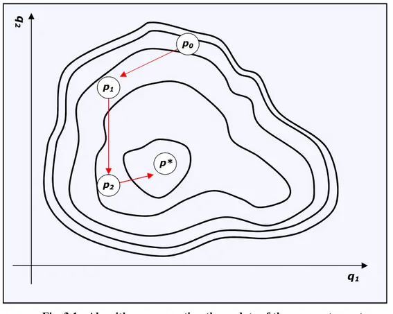
Fig. 3.1 - Algorithm representing the update of the parameters set p
Essentially, 3 steps have to be followed to update the parameters. First, an opportune approximation Fa of the function is computed; second, based on the approximation just done, a search direction d is chosen; third, the step length α in direction d is chosen, to find the new set:
The procedure of choosing the step length α is known as line search. Another approach similar to the line search is the use of a trust region. This is the region in which the approximation Fa holds sufficiently true. The direction d is chosen only if a step in that direction is still inside the region. For more information on this procedure, not used during the thesis, see ref. [3], [16] and [18].
d α + p = pi+1 i ⋅ Eq. 3.29 q1 q 2 p0 p* p1 p2
26
3.6.1 Sequential Quadratic Programming
The previous paragraph describes how NLP solvers’ algorithms attempt to near minima of the performance index. A more in-depth description of a very widespread algorithm, the Sequential Quadratic Programming (SQP) [12] [13], will be provided. For the sake of simplicity, the augment constraint c~E will be simply indicated as cE from now on.
As the name suggests, SQP approximates the performance index up to second order and the constraints up to first order in an interval of p. Then, if d is a perturbation of p:
d p H(p) d + d (p) g + F(p) d) + F(p T T d d 2 2 0.5 min min ∂ ∂ ≅ 0 = d (p) C + (p) c d) + (p cE ≅ E E 0 ≤ ≅c (p)+C (p)d d) + (p cI I I Eq. 3.30
the problem above is called Quadratic Programming (QP) problem. In analogy with the NLP problem, the QP problem optimality conditions are:
0 0 0 2 2 ≤ − ∂ ∂ I I E E T c + d C = c + d C = λ C g + d p H 0 0 = ) c + d (C λ λ i I, i I, i E, I ≥ Eq. 3.31
The procedure to follow for solving QP problems is known as active set strategy [11]. Let’s arbitrarily assume that mIS of the mI inequality constraints are satisfied with the equal sign by the solution d* of the QP, i.e. they belong to the active set, and discard the others. The QP problem has now changed in an Equality Quadratic Problem (EQP) in the form:
0 0 2 2 = c + d C = g + d p H AS AS ∂ ∂ Eq. 3.32
where cAS and CAS are the active set’s m constraints and Jacobian.
The second of eq. 3.32 represents a linear equation system of n unknown in m equations, with ∞(n-m) possible solutions of d. The generic solution can then be written as:
t Z + d = d 0 Eq. 3.33
where d0 is a particular solution of the system, t is an arbitrary vector of length n-m and Z is an n·(n-m) matrix with columns that are bases of ker(CAS).
27
Substituting the expression of d of eq. 3.33 in the first of eq. 3.32 yields a simple first order equation: 0 0 2 2 2 2 = d p H + g + t Z p H ∂ ∂ ∂ ∂ Eq. 3.34
that can be easily solved since no constraints have to be satisfied. Once t is found, d follows immediately from eq. 3.33.
Note that, since d was yielded from an EQP in which the active set was arbitrarily guessed, this solution is not the exact solution of the QP but just an intermediate solution that satisfies the given active set.
Updating the current point pk straight away: d + p =
pk 1+ k Eq. 3.35
would yield a new point pk+1 that it’s surely feasible with respect to the active set, but that may not satisfy the inequality constraints that are excluded from the active set. To prevent this, step in direction d is reduced by a factor α as seen in eq. 3.29. Put the inequality constraint in the following form: = mI I I I C C C , 1 , M = mI I I I c c c , 1 , M Eq. 3.36
If CI,j e cI,j don’t belong to the active set, for p k+1
to satisfy the constraint it must be:
j I, j I, k j I, + k j I, p =C p +C αd c C 1 ≤− 1 0<α≤ Eq. 3.37
The inequality constraints out of the active set for which we have α<1 are called blocking constraints: these are the inequality constraints that would be violated if the entire step d would be taken.
Of the blocking constraints, the algorithm selects the one corresponding to the lowest α and adds it to the active set. This is the constraint that is encountered “first” while moving from the starting point along the direction d.
Another modification of the active set is done by checking the fourth of eq. 3.31:
λI , i≥ 0 Eq. 3.38
for each of the active set’s inequality constraints. If the correspondingλ does not satisfies the I,i
28
Now, with the active set changed as above, another EQP problem is solved starting from the now surely feasible updated point pk+1:
αd + p = pk 1+ k Eq. 3.39
Following this procedure, not only the parameters’ set p converges to the solution, but also the active set gradually converges to the solution’s active set.
The SQP method didn’t enjoy immediate success among numerical application after its ideation and was overshadowed by other numerical methods (such as the Penalty function or the Barrier methods) because of the difficulty of computing, for each step, the Hessian of the Hamiltonian. New interest in the method aroused after methods of approximating the Hessian were developed; in particular the ideation of the Quasi-Newton approximation [20] has been a major step in applicability of this method.