S e c t i o n 2 .
IMPROVING THE MODELLING OF TWF
In the following paragraphs a new analysis will be introduced whose aim will be to improve the starting TWF Solid model. As discussed in Section 1, the starting TWF yarn is interpreted with a geometry made up of only straight parts and modeled with Solid HEX8 elements; the connection between the cross region and the free part of the yarn is interpreted without taking care of the curve shape that the yarn has in the reality; not only, but according to the three yarn directions 0, + 60, - 60 which characterize the single RUC cell, three different groups of elements were defined of which the material properties were related to Coordinate Systems defined with a fixed orientation and so not able to let the properties follow the real shape of the yarn through the weave; these are all drawbacks referred to the existing model. According to these problems it will be introduced a new geometry of the yarn, an appropriate material property definition and it will be introduced a new set of models built in different ways in order to understand which one is able to reproduce faithfully the mechanical behavior of a TWF specimen. Each model will be created in PCL language so it will be possible to change the geometry of the single RUC and the size of the specimen just by changing directly these values in the PCL function. As it was said, it will be also introduced a mechanical simulation test in order to evaluate the E1 modulus of each model and results, comparisons and comments will be added at the end of this section.
1
SOLID ELEMENT TWF MODEL
The new TWF model introduced in this paragraph is built by using Solid HEX8 elements. It will represent more closely the Superelement 2 of Hoa and Zhao [1], which is characterized by the use of curve sine functions to model the free part of the yarn. The model that will be now introduced is based on the following assumptions:
• Cross region modeled as rectangular
• Twisted configuration of the yarn
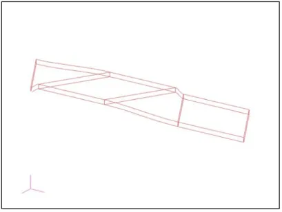
The following picture shows the new geometry set. It is important to underline that because of the sine curves introduced between the cross parts of the single yarn, this new configuration has bigger slopes than the starting one made up of only straight parts everywhere.
Figure 1: New yarn geometry.
After this first step, the same kind of solid elements will be used to mesh the new yarn; in particular it will be used a different number of meshseed (meshseed is the number of nodes which has to be defined on each curve of the geometry according to which the mesh of all the volume will be built) according to the cross region or to the connectivity region of it. In the following pictures it will be possible to follow all the steps performed to arrive to the new single RUC cell definition. Looking at the new definition of the yarn it was decided to maintain two HEX8 elements through the thickness. In the cross region it was defined a total of 8 HEX8 elements while in the connection region, because of the sine curve parts, it was decided to increase the number of Solid elements in order to have a faithful interpretation of it. In the following pictures it is possible to look at the final yarn configuration.
Figure 3: New yarn solid model.
Figure 4: Zoom of the connection slopes
As it is possible to see in the pictures above the new model has twenty four HEX elements on each curve part instead of the eight elements used in the starting model; so the new yarn is now made up of
64 HEX8 elements. A convergence study was performed by splitting each HEX element into 8, but comparing the E1 modulus prediction no significant difference was revealed so it was chosen to consider six HEX elements on each curve side considering it as a reasonable number of elements able to reproduce faithfully the real shape.
Figure 5:Detail of the mesh approximation of the slopes.
According to the new yarn definition, a second improvement will be now introduced. As it was said in the introduction of this chapter, the starting finite element model was characterized by three groups of properties whose elements had properties defined according to the Correspondent Coordinate System according to the yarn directions 0, +60, -60 degrees. Each C.S. was defined with a fixed direction which doesn’t depend on the shape of the yarn. In this way all the three groups of elements had properties which were not able to follow the shape of the correspondent interlacing direction of the yarn through the weave. Two options of C.S. that are available in NASTRAN were considered: 1) The definition of local coordinate frames which define the correct material orientation. 2) Defining the HEX elements in order to have the element coordinate system aligned with the correct orientation. Option1: instead of a Coordinate System a Local Element Coordinate System could be created and the material properties could be defined according to the new coordinate system. In this way each HEX element could have its own local coordinate system with the x direction oriented in the yarn direction. In that case since the yarn could be considered transversely isotropic, orienting the x-direction of the C.S. parallel to the yarn direction would be sufficient for a correct definition of the material properties. Otherwise if the material is not transversely isotropic, in addiction, the y-axis of the local C.S. has to belong to the plane
of the yarn and the other one normal to it. Due to the difficulty to define in this way a correct coordinate system, it was chosen to follow the option 2.
Figure 6:particular of the original local element system of the yarn
Option 2: the orientation of each element is aligned to the orientation of the created geometry. Due to complex shape of the geometry, it was not always possible to create solids whose HEX elements have correctly oriented local C.S.. We can see in the picture above that to define a right oriented local system was a really difficult work because each element had its own orientation and it changed going from the straight part of the yarn to the curve one. This problem was in part solved working directly on the orientation of each HEX element and reversing it; in this way it was possible to define a correct orientation only for the straight part, but not for the curve part of the yarn; to change the orientation in the curve part it was necessary to change the connectivity of each HEX element which belonged to that region. Figures 8-9 show the final right oriented local element system that will be used to define in the right way the material properties of the yarn.
Figure 8: Final yarn local element system.
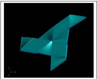
According to this final yarn configuration, it is now possible to define in the correct way the material properties; now instead of the three groups of elements created in order to define the material properties according to three different Coordinate systems, the new model will have no groups of properties because in NASTRAN the element C.S. used for the material properties orientation unless a C.S. is specifically assigned. After the two steps explained above to create a single RUC cell it was sufficient to define a group made up of the single yarn, to copy it two times and to rotate each copy; the result is the new single RUC cell shown in the picture below.
Figure 9: Single RUC cell.
According to all that was said before, now the new RUC cell will have the following set of element coordinate system.
Figure 10: Particular of the cross region.
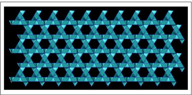
Now it is possible to go on and to define the final TWF specimen that will be subjected to mechanical tests in the following part of this Section 2. In fact it is enough to define a group made up of one single RUC cell and to repeat it according to the value of the Width and the Length in terms of number of RUC single cells. In the following picture it is possible to look at the total TWF specimen; it is important to underline that this new solid model is automatically defined thanks to a PCL function that
will be introduced later; in this way it is enough to give in input the values of the Width and of the Length to obtain automatically the correspondent specimen; it is the same if is necessary to change the geometry of the single cell. But for this it is important to define the new geometry according to the same parameters introduced in the PCL function. These geometrical parameters are the same of the previous setting.
Figure 11: Total TWF specimen.
1.1
Testing the Solid Element Model.
In this paragraph it will be performed a mechanical test in order to evaluate the E1 modulus of a 6x6 cell TWF specimen according to the new solid model introduced in the previous paragraph. The material is a transversely isotropic Carbon Epoxy composite. In order to compare the new results with the old ones, it will be considered a TWF specimen configuration with no free edges.
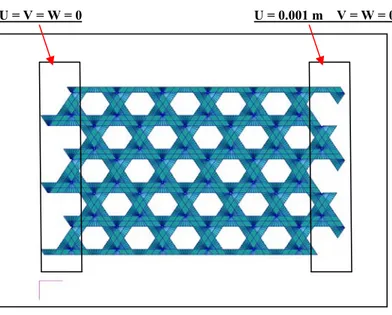
The boundary conditions that will be applied are the same introduced in Section 1 and used in G.Palermo’s work, so in this way it will be possible to compare the new results to the old ones. In the detail the left side of the specimen will be fixed, while on the opposite side a displacement of a given intensity will be applied; again the y and z displacements will be fixed to be zero. The following picture shows the configuration.
Figure 12: boundary conditions
U = V = W = 0 U = 0.001 m V = W = 0
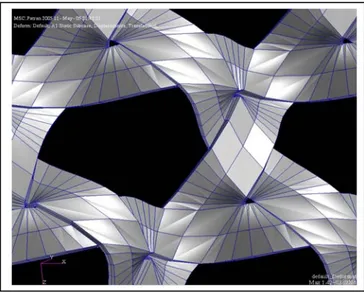
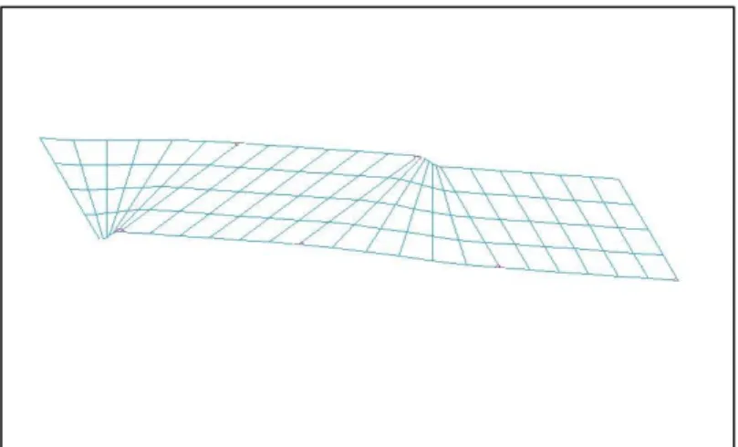
In the following picture it is possible to see the deformation of all the specimen under the applied boundary conditions and a particular of the cross region; the results evaluated in terms of Fx-reaction on the fixed size and E1 modulus are shown below.
Figure 14: Particular of the RUC deformation.
Figure 15: particular of the deformation of the cross region
Looking at the pictures above it is possible to see what happens in the model during the deformation; the single RUC cell is really subjected to deformation out of the plane and a twist is involved too; in fact the single RUC seems to be quite subjected to a torque around the X-axis; not only, but if the attention is focused to the rectangle to which the red arrow in the picture is related, it is also possible to see that the big slopes are the reason of the big step on the corner side of the cross region. This is also
the reason of the non homogeneous deformation of all the side of the yarn involved in the cross region.
• Evaluation of the E1 modulus.
According to the same way used in the previous tests to evaluate the E1 modulus, the following formula will be used.
E1 = Fx * L / ( W * t * u)
Where Fx is the reaction in the x direction evaluated on the fixed side of the specimen using the utility tool summation, L is the free length of specimen, W is the width of the specimen with no free edges, t is two yarn thicknesses and u is the displacement applied on the right sight in the x direction. The values obtained in terms of reaction and E1 modulus are shown below.
• Global system : Fx = - 3.1353 N; E1 = 25.8660 Gpa
This result is obtained referring the material properties to global coordinate systems as well as in the starting finite element model; it is interesting to look at the new results obtained with the new Local Element Coordinate System.
• Local system : Fx = - 1.4702 N ; E1 = 12.129 Gpa E1
The results obtained with the present analysis show that there is a large difference in the predicted behavior of the fabric if the two kinds of material definition are used; in particular the results obtained according to the local element system are really low while this should be the correct way to define the material properties. Because of this, many checks were performed to the new FEM; in particular the geometry definition, the local element system definition and the mesh used on the model were checked but no errors were found. To further investigate this it was decided to develop shell element models in which the use of shell elements reduce the yarn geometry to the mid plane itself. Assigning correct
material orientation is simple because the material is introduced defining a laminate composite whose layers are related to the middle plane of the yarn cross section and defined in terms of thickness value and material properties. After that each shell elements will have properties whose orientation will be defined projecting the x-axis of the reference coordinate system on the surface of the element (See appendix A). In this way it will be possible to compare the results to the ones obtained with the previous solid model defined with material properties related to the local C.S.. Because of working with the middle plane, the new models will need a new interpretation of the cross region; in fact it will be necessary to impose the relative displacements of all the nodes with the same x-y coordinate to be zero through the thickness. For this three options were considered:
1. Rbe2 elements. 2. Solid elements.
3. Solid and Rbe2 elements.
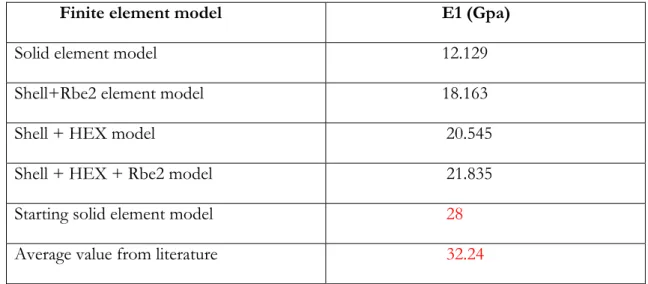
According to these three options, three models were built and subjected to the same mechanical simulation performed in the previous analysis, maintaining the same boundary conditions. The following table summarizes the results obtained in terms of E1 modulus.
Finite element model E1 (Gpa) Solid element model 12.129 Shell+Rbe2 element model 18.163 Shell + HEX model 20.545 Shell + HEX + Rbe2 model 21.835 Starting solid element model 28 Average value from literature 32.24
Table 4: Comparison of the E1 modulus results
The table above shows that through all the new models there is some difference; in particular it is possible to see that the solid model has the lower value of stiffness, while shell models have values which belong to a range of 3 Gpa starting from 18.2 Gpa. But it is interesting to underline that despite
all, these values are still far from both the starting model E1 value and the average value available from literature. Because of this, a new analysis was performed working directly with the starting solid model; in particular it was defined a local coordinate system and a fragment of specimen was subjected to the same mechanical simulation of the previous analysis. The results revealed that also the starting model was characterized by the same strange behavior discovered in the new solid model. Not only, but reading the documentation from which both the previous and the present work start, there is an unclear definition of the parameters that are used in the E1 modulus formula. In particular in the documentation the E1 modulus value is evaluated according to the nominal thickness of the TWF specimen, but there is no reference about the way the nominal thickness is evaluated, so a faithful comparison cannot be performed because of this. In fact instead of the nominal thickness as mentioned in the documentation, all the values obtained in the present and in the starting work of G.Palermo are linked to a two thicknesses value, so a comparison will be surely affected by an error. According to this, since no errors were found in each FEMs and since the results obtained with both solid and shell models were comparable, but far from the real one, additional investigations were done. In particular thanks to Cambridge University which worked on TWF modeling the TWF using only beam elements, it was possible to use its data base, so, thanks to this, a clear definition of all the parameters involved in the E1 analysis was available. Before trying to correlate the developed models to Cambridge results, additional investigations were done working directly on a single yarn. In particular it was studied the rule of the shape used to model the yarn itself defining a beam model and the correspondent solid element model. It was considered the case of a non twisted yarn, the same mechanical simulation was performed and the results revealed that the rule of the shape is significant in the reduction of the stiffness. In particular more the shape is regular and symmetric, more the stiffness value is high; on the other side, more the slopes are big, more the stiffness decreases. Not only, but working with a non twisted yarn, the solid model gives more or less the same values of the beam model both according to the local element C.S. and the C.S.. Because of this, a test was done defining a twisted yarn (exactly like the real one) and working with solid elements; the result was that the values obtained with the two C.S. are really different, revealing that the contribution of a twisted yarn configuration to the decrease of the stiffness is significant; not only, but more the slopes involved are big, more the reduction of the stiffness is high and more the difference of the results is big using the two C.S... Because of this, and thanks to micrographs of the yarn, it was possible to see that a large slope as in the solid model, caused by assumption of rectangular cross section, is not realistic. According to this, a new shell model was developed defining a new yarn geometry characterized by lower slopes as the real ones that the yarn should have because of a lenticular section of it. It was decided to use a Shell element because due to the difficult new geometry set, it is impossible to model the new yarn in PATRAN using solid elements; for this it is suggested to use other programs like
CATIA. The new model was built introducing Rbe2 elements in all the cross regions of the RUC and the same mechanical simulation performed by Cambridge University was followed. As it will be shown in the next paragraphs, the results obtained show that the comparison with the Cambridge results is really good and the new shell model finally well simulates the real mechanical behavior of the TWF.
2
SHELL ELEMENT MODEL WITH RBE2 ELEMENTS
In this new paragraph a new model will be introduced; it will be built using only shell elements and introducing Rbe2 elements in the cross region of the RUC. As it was done in the previous solid model, the new Shell+Rbe2 model will be created defining a PCL function which will be able to define a general TWF specimen by introducing the size of the specimen itself in terms of number of RUC cells that identify the Length and the Width of the specimen. Again it will be also possible to change the single yarn geometry. The material properties introduced refer to a 2D-ORTHOTROPIC MATERIAL and a composite laminate was introduced made up of two layers with thickness equal to 0.035 mm; this is because the Shell geometry is created in terms of the middle plane of the single yarn. In the following table it is possible to check the material properties used.
Table 1: 2D-transversely isotropic material properties
According to all that was said above, a new geometry is now introduced in order to identify the middle plane on which the shell elements will be defined. The new geometry will continue to consider the yarn as made up of straight parts on the cross region and curve sine parts on the connection region.
The following pictures will show the new geometry that will be considered as reference for all the other shell models that will be introduced later.
E11 E22 Poisson ratio 12 Shear M. 12 Shear M.23 Shear M.13
Figure 16: New geometry set.
Once defined the mid plane it is possible to mesh each surface and define in it the correspondent Shell elements; it was chosen to define CQUAD4 elements in each surface of the yarn. Figure 19 shows the configuration.
Figure 17: CQUAD4 Shell elements.
As it is possible to see from the picture above the new shell yarn is made up of 24 shell elements in both the curve and the straight parts of the yarn. The same steps introduced with the solid element model will be followed in order to define the single RUC cell and then the specimen itself. It is important to underline that, because of the use of Shell elements, it is necessary to introduce Rbe2 elements in the cross region in order to impose the relative displacement of the nodes with the same x-y coordinates of two different x-yarns to be zero. In particular all the relative degrees of freedom will be
impose to be zero. The following pictures will show both the single RUC cell and a zoom of the cross region.
Figure 18: Single RUC cell.
Figure 19: particular of the cross region: the red arrows indicates a Rbe2 element.
2.1
Testing the Shell Element Model.
In the following paragraph the new shell model will be subjected to the same mechanical test used with the solid element model; the E1 modulus test. In particular, the same boundary conditions will be applied and the results will be evaluated in terms of Fx-reaction on the fixed side of the specimen and the same E1 formula will be used. According to the previous tests it will be considered as reference a configuration characterized by no free edges inside. The pictures below show both the specimen with no free edges, the boundary conditions applied on it and the deformation with a particular of the cross region.
U = V = W = 0 U = 0.001mm V = W = 0
Figure 22: particular of the deformation of the cross region.
As it is possible to see in the picture above, this new configuration is characterized by the presence of a strange behavior in each cross region especially where it is indicate with the red arrow. The reason is that the cross region of two different yarns is not defined with Rbe2 elements in each correspondent node. In fact the cross region is only made up of 4 Rbe2 elements, one for each corner side of it, so the remaining part of it has no constraints and so it is free to deform. In particular there is something like a compenetration of the middle part of the cross region. It could be suggested to define Rbe2 elements in all the cross regions of the RUC single cell. The results obtained in terms of the Fx-reaction and the E1 modulus (it was used the same E1 formula as in the previous tests) are shown below.
• Fx = - 2.2017 N • E1 = 18.1638 Gpa
As it is possible to see from the results, both solid and shell model give values comparable but still far from the average value found in the Quebec documentation.
Table 2: comparison of the E1 modulus results.
Finite element model E1 (Gpa) Solid element model 12.129 Shell+Rbe2 element model 18.163 Starting solid element model 28
Looking at the table above, it is possible to see that the actual two models have E1 modulus quite far from the starting Solid element model of the previous work and also from the average value of E1 = 32.3 Gpa available from literature thanks to the University of Quebec Montreal documentation. Not only, but looking at the results of the new two models it is possible to underline that they are absolutely comparable because the difference belongs to a range of more or less 6 Gpa; it means that the inconsistent value obtained with the new solid model according to a local element system is verified by the Shell model, so the behaviors of the two models should be correct. It remains to answer to this new question: ”Why the new models have a low stiffness?”. To solve this new problem, in the following part of the paragraph new models will be created according to different ways to interpret the cross region of the single RUC and the yarn itself. The same mechanical test will be applied to them according to the same boundary conditions; again, it will be considered as reference a configuration with no free edge and the dimension of the specimen will be maintained equal to 5x6 RUC cells. The results will be evaluated in terms of the Fx-reaction on the fixed side of the specimen and in terms of E1 modulus.
3
SHELL AND HEX ELEMENT MODEL.
In this paragraph a new model will be developed. It will be made up of shell elements for the yarns, but the cross region will be modeled with Hex elements defined with the resin properties. It is an unreal simulation because in this way in the cross region there is more resin than the real quantity; anyway it is a good example in order to understand the rule of the resin in the TWF specimen behavior. Again the impregnated property of the composite is the same as well as the boundary conditions applied on the model. According with the iter chosen in the other models it will be considered a no free edge configuration. The following pictures will show the configuration.
Figure 24: RUC cell.
In the picture above it is possible to see the cross section; it was used one hex element through the thickness instead of the RBE2 elements. It is clear that the results will be higher than the last Shell and RBE2 elements because of the resin presence in each cross section; in fact this new configuration implies a surplus of resin in the cross region if compared to the reality. The following pictures show the same E1 modulus test applied on a 5x6 RUC specimen and the results in terms of reaction on the fixed side and E1 modulus.
Figure 26: Deformation of the model.
In the following picture it is possible to see the particular of the deformation in the cross region of this model.
Figure 28: zoom of the cross region
As it is possible to see above, there is something like a step in each corner size of the cross region; the reason is related to the hex elements that were introduced instead of the rbe2 elements; in fact in this way it was not fixed the relative displacement of the nodes which belong to the cross region. The cross region will behave according to the resin properties so the step is caused by the deformation of the resin under the displacements involved by the two yarn deformation. In other words the resin introduced represents a softer constraints than the Rbe2 elements with which it was possible to impose the relative displacement of the correspondent nodes to be zero.
According to this, the results obtained are shown below:
• Fx = - 2.4903 N • E1 = 20.54481 Gpa
As it is possible to check, this new E1 modulus value is higher than expected, but not so much if compared to the E1 modulus obtained with both the first solid and the Shell+RBE2 model. This is another important prove of the fact that the new models are well done; in fact all the results belong to a range of 8 Gpa.
4
SHELL +HEX+RBE2 MODEL.
According to the results obtained with the last model it will be introduced the last model of this long and detailed analysis; again the material used will be the same as well as the boundary conditions applied. This new model should be the stiffest of the other models; it will be built using Shell elements for the curve parts of the yarns, Hex elements with transversely isotropic property in each cross region and RBE2 elements introduced to impose no relative displacements in the cross region to. The following pictures will show in the detail this new model. As it was done for all the other models, this new model will be created defining a new PCL function. According to this it will be shown now the new interpretation of the geometry and the new yarn that will be modeled with shell elements in each connection region and HEX8 elements in each cross region. The following picture shows the new geometry.
Figure 29: New geometry set.
In the picture below it is possible to see the single yarn with all the mesh on it made up of Shell elements and Solid elements and the two material property sets; in particular in white is represented the 2d-orthotropic material used in the shell elements while in red is represented the transversely isotropic material used in the cross region defining hex elements.
Figure 30: new material property set.
According to the same method used to create the previous models, starting from the final yarn configuration it is possible to create the single RUC cell and then the total specimen itself. The pictures below show all the steps and a particular of the cross section modeled with Hex and Rbe2 elements is shown to.
Figure 32: particular of the cross region with hex and Rbe2 element; the arrow indicates a Rbe2 connection.
In the picture above it is possible to look at the particular definition of the cross region; in fact now there are four layers of Hex elements defined with transversely isotropic material and the rbe2 elements are introduced in order to impose the relative displacement of each hex element to be zero. In this way the model should be more faithful than the others introduced in this same section because it is made up of shell element and a very detailed cross region which should simulate in a good way the real behavior of the TWF. The following pictures show the total specimen obtained again in the cut edge configuration.
The same boundary condition will be applied: the left side of the specimen will be fixed in all the degrees of freedom while in the opposite side a displacement in the x direction of 0.001m will be applied. In the following picture the deformation of the model is shown.
Figure 34: deformation of the model.
The results obtained with this last E1 modulus test are shown below.
• Fx = - 2.64675 N • E1 = 21.83550 Gpa
This was the last model introduced in this section. For comments on the improvements obtained and on the results, it is appropriate to start from the initial solid model. An E1 modulus of 28 Gpa was found with a model made of small number of HEX elements, with no curved parts defined in it and with a property system which is not able to follow the shape of the yarn. This value is quite close to the real one available from literature. Starting from this point, a new solid model has been introduced; it was built as faithful as possible to the real geometry, with a larger number of HEX elements, with curve
parts and defining a property set which is able to follow the shape; the result shows a large difference starting from the original C.S. (25 GPa) and going to the new local element C.S. (12.2 GPa). In order to find the reason of this strange behavior new models were introduced; Shell+ RBE2 element model, Shell+Hex model and Shell+Hex+RBE2 model. The values obtained with these models fall in a range of 2 or 3 Gpa starting from 18.8 to 21.8. These results are comparable with the first one obtained with the solid model 12.1; the difference with the solid model value and the shell model value is quite large, but not so far if compared to 32.2 Gpa which represents the real value. Since no errors were found in the models introduced, in the next paragraph the same procedure of defining a local element coordinate system will be applied directly to the old starting Solid model and a new test on a part of it will be performed.
5
TESTING THE STARTING SOLID MODEL.
In this new paragraph only a small part of the old starting solid model will be considered; the total specimen was not defined in order to take care of a local element coordinate system, so the work required to adapt it to this new Coordinate system is too big and difficult. In the following pictures the portion of model that will be considered in the next analysis will be shown.
The first problem to solve is to adapt this fragment to a Local element system; it was really a quite difficult work because it was unknown how this model was defined. Using reverse of the system and changing the connectivity it was possible to find the right coordinate system defining three different groups according to the three directions of the TWF; all the procedure is shown in the next pictures step by step.
• Zero direction group
• + 60 degree direction.
• - 60 degree direction.
Figure 37: +/- 60 direction group
• Final result with the correct local element coordinate system.
Figure 38: final correct oriented local element coordinate on the starting solid model.
According to the model above, the same boundary conditions used in the last test will be applied: the left side will be fixed while a displacement will be applied on the right side. The following pictures show the configuration.
u = v = w = 0 Figure 39: boundary conditions u = 0.001 ; v = w =0
The results are shown below in terms of reaction evaluated on the fixed side of the specimen.
• Fx = -2.221 GLOBAL COORDINATE SYSTEM • Fx = -1.257 LOCAL ELEMENT SYSTEM
This is the prove that the starting model had the same strange behaviour of the new solid model that was introduced at the beginning of this Section.
But now a new problem has to be solved; why this behavior? One of the reason that can in part justify this behavior is a non correct definition of the nominal parameters which were considered as reference of the model. In fact, reading the following rows it will be possible to understand that actually there is an unclear definition of the nominal thickness used in the E1 formula introduced in the Hao and Zhao [1] documentation.
(this is an extract taken from the Hao and Zhao [1] documentation)
“The cross section area is obtained as the product of width and thickness. Due to the ondulation of the TWF there can be many cross section areas. This is due to the fact that at some location, the thickness consists of only one-yarn thickness while at other locations, the thickness consists of two-yarn thicknesses. Therefore there can be four different thicknesses: those corresponding to one-yarn thickness, two yarn thicknesses, the average (obtained by the weighted average of the one-yarn thickness and the two-yarn thicknesses) and the nominal (obtained by measuring the TWF sheet using a micrometer). The width is obtained by direct measurement on the sample using a micrometer. The nominal cross section area based on measured thickness and measured width is used here.”
Reading the rows above it is important to underline that actually in the tests performed until now, a two-yarn thicknesses of 0.14 mm was considered; it means that we are not considering the nominal thickness value as it is indicated in the documentation. According to this, it is clear that the influence of a different thickness is very large as it is possible to check in the E1 formula used in the test. The problem is that there is no nominal value indicated in the Quebec documentation and no answer was received about the request of nominal values to use in the PCL function. Just to underline the effect of a different thickness value in the E1 modulus evaluated in each model, we could consider a 0.10 mm thickness (it is something like an average but just chosen as example); the results in terms of E1 modulus are shown below:
thickness = 0.14 mm thickness = 0.10 mm
E1 modulus (GPa) E1 modulus (GPa)
Solid HEX8 model 12.129 20 Shell + RBE2 model 18.1638 25.42 Shell + HEX8 model 20.54481 28.7 Shell + HEX8 + RBE2 21.83550 30.57
Table 3: comparison of the E1 results with different nominal thickness.
The table above shows the influence of the thickness value on the E1 modulus; as it is possible to check, a small difference in the thickness value involves a large difference in the results. Since we have no indication about the thickness value used in literature, a true comparison of the results cannot be performed. A true comparison can be done only if same values are used. Adding comments about the four TWF models introduced in this section, we can only say that a comparison between them shows that the solid HEX8 element model seems to have not enough stiffness; since no errors in the FEM were found, additional analysis will be added in the next Section. In particular, the data base, kindly provided by the Cambridge University and in particular Prof. Eng. Pellegrino, will be analysed; Cambridge University worked on TWF developing a model made up of beam elements, mechanical test were done directly on one configuration of TWF specimen, simulation with the beam models were done, so it will be possible to adapt the RUC geometry that was used to the new models introduced in this Section and in particular to the Solid model and the Shell model in order to understand the reason of the inconsistent values obtained with the previous analysis and to compare the new results according to a clear definition of all the parameters that are involved in the contest.