Chapter 6
Rear-Wheel Drive Car simulations
In this chapter we present the results provided by the simulations, with regard to a rear-wheel drive car, in the next chapter we deal with a front-rear-wheel drive car. In all the simulations we impose open-loop steer angles; we define the steer functions before running the simulations, and they are not affected by the vehicle motion. Therefore the driver in-puts depend on the instantaneous vehicle behavior whereas man-car-external environment constituted a closed-loop system.
In this report we refer to a vehicle equipped with tyres which size is 195/65-R15. The vehicle model we analyzed to define the Active Yaw Control set-up was provided with a set of tyre parameters obtained testing this tyre. We simulated also a car supplied with tyres 205/55-R15, without changing the PI controller, in order to understand if an ESP and redistribution of torque controller allows to obtain good results even if its set-up is at first developed for another type of tyre. Some simulations regarding the car provided with the sport tyres are illustrated in the “Appendix A” and in the “Appendix B”. The M-file in which are included the tyre and car parameters is reported in “Appendix C”.
6.1
High Speed A
The first simulation illustrates condition in which the driver wants to drive along a too sharp curve, considering the car speed. The speed in fact is, before starting the cornering
manoeuvre, close to 55 m
s (almost 200
km
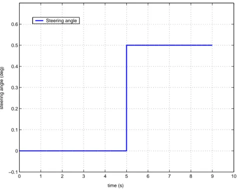
h ), and the steer angle follows a step function,
represented in fig.6.1. The final value is 0.5 deg, and supposing a steer transmission ratio equal to 1:20, it corresponds to an angle, applied by the driver to the steering wheel, equal
0 1 2 3 4 5 6 7 8 9 10 −0.1 0 0.1 0.2 0.3 0.4 0.5 0.6 time (s)
steering angle (deg)
Steering angle
Figure 6.1: Steer angle function
with the ESP, and provided with the “Haldex” coupling. We tried also to simulate the combined effects of the ESP and redistribution of torque but in that case the ESP system does not act.
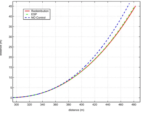
Analyzing the trajectories the cars drive along (fig.6.2) we can understand that our stability control detects an oversteering manoeuvre. The trajectories which the two cars provided with the stability systems follow in fact are wider than the bend driven along by the uncontrolled vehicle. However we can realize better the real effect of the stability systems comparing the “R” distance and the body slip angles (β) in the three cases (fig.6.3 and fig.6.4)
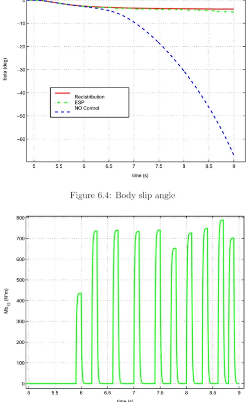
If the car is not provided with any Active Yaw Control it looses stability and it spins around. We can understand this fact since the “R” distance decreases too much, approach-ing zero, and |β| becomes bigger and bigger. Observapproach-ing fig.6.3 we want to point out that using a stability system we manage to keep an average curve radius close to the reference radius, but we do not reach a stable steady state condition. Also the β angle remains quite small, and it does not exceed -10 deg (if the body slip angle becomes lower we decided to consider the simulation failed because in a car following that motion a driver would not feel safe). In order to achieve this goal we activate the brake system and the central coupling in the way shown in fig.6.5, 6.6, 6.7.
300 320 340 360 380 400 420 440 460 480 0 5 10 15 20 25 30 35 40 45 distance (m) distance (m) Redistribution ESP NO Control
Figure 6.2: Trajectories driven by the three vehicles
5 5.5 6 6.5 7 7.5 8 8.5 9 100 200 300 400 500 600 time (s) corner radius (m) Redistribution Reference radius ESP NO control Figure 6.3: “R” distances
5 5.5 6 6.5 7 7.5 8 8.5 9 −60 −50 −40 −30 −20 −10 0 time (s) beta (deg) Redistribution ESP NO Control
Figure 6.4: Body slip angle
5 5.5 6 6.5 7 7.5 8 8.5 9 0 100 200 300 400 500 600 700 800 time (s) Mb 12 (N*m)
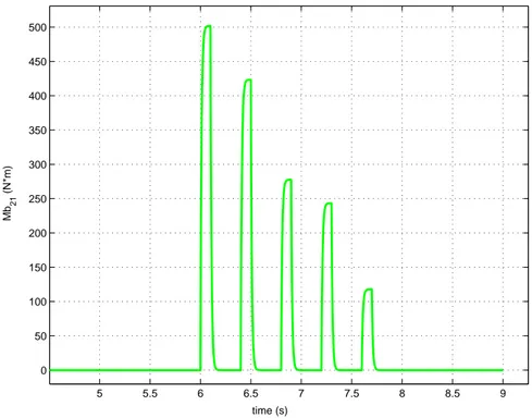
5 5.5 6 6.5 7 7.5 8 8.5 9 0 50 100 150 200 250 300 350 400 450 500 time (s) Mb 21 (N*m)
Figure 6.6: Brake torque applied to the rear inner wheel
4.5 5 5.5 6 6.5 7 7.5 8 8.5 9 0 0.1 0.2 0.3 0.4 0.5 0.6 0.7 0.8 0.9 1 time (s)
valve (1 closed; 0 open)
We want to remark the fact that both an ESP action (with regard to the front outer brake (fig.6.5)) and a redistribution of torque action (fig.6.7) match with a “R” distance and a β angle that increases. In reference to the rear inner brake (fig.6.6) we can notice that it is never activated simultaneously with the front brake, and the brake torque is lower and lower during the simulation, and after few time it becomes null. The effect of this braking action is to damp oscillations that the ESP would trigger during the first instants of the manoeuvre if it acted on only one brake.
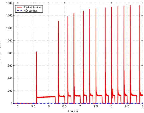
The intervention of the “Haldex” system causes a torque directed towards the front axle which is reported in fig.6.8 (this is the torque provided by the coupling, before the differential gear box).
5 5.5 6 6.5 7 7.5 8 8.5 9 0 200 400 600 800 1000 1200 1400 1600 time (s) Torque front (N*m) Redistribution NO control
Figure 6.8: Drive torque provided to the front axle
Except for the first instants after the valve closing, during which we have very high peaks, that in any case decrease so quickly not to have significant effects on tyre perfor-mances, the car reaches a condition in which the amount of transferred torque is almost constant while the valve is closed.
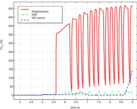
In this first simulation we illustrate also the tyre performances, to stress the effects of this two stability systems on the forces which the car motion is due to.
Without using any control system we can notice the fact that the forces transmitted by the inner tyres become zero after almost 7 s (fig.6.11, 6.13, 6.15), and it means that the
4 4.5 5 5.5 6 6.5 7 7.5 8 8.5 9 0 50 100 150 200 250 300 350 400 450 500 time (s) Fx 11 (N) Redistribution ESP NO control
Figure 6.9: Longitudinal force transferred by the front inner tyre
4.5 5 5.5 6 6.5 7 7.5 8 8.5 9 −3000 −2500 −2000 −1500 −1000 −500 0 500 1000 time (s) Fx 12 (N) Redistribution ESP NO control
4.5 5 5.5 6 6.5 7 7.5 8 8.5 9 −800 −600 −400 −200 0 200 400 600 800 1000 time (s) Fx 21 (N) Redistribution ESP NO control
Figure 6.11: Longitudinal force transferred by the rear inner tyre
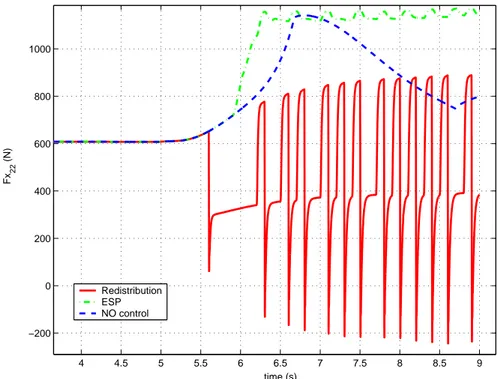
4 4.5 5 5.5 6 6.5 7 7.5 8 8.5 9 −200 0 200 400 600 800 1000 time (s) Fx 22 (N) Redistribution ESP NO control
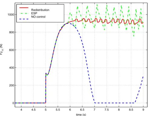
4 4.5 5 5.5 6 6.5 7 7.5 8 8.5 9 0 200 400 600 800 1000 time (s) Fy 11 (N) Redistribution ESP NO control
Figure 6.13: Lateral force transferred by the front inner tyre
5 5.5 6 6.5 7 7.5 8 8.5 9 0 500 1000 1500 2000 2500 3000 3500 4000 4500 5000 time (s) Fy 12 (N) Redistribution ESP NO control
4 5 6 7 8 9 0 100 200 300 400 500 600 700 800 time (s) Fy 21 (N) Redistribution ESP NO control
Figure 6.15: Lateral force transferred by the rear inner tyre
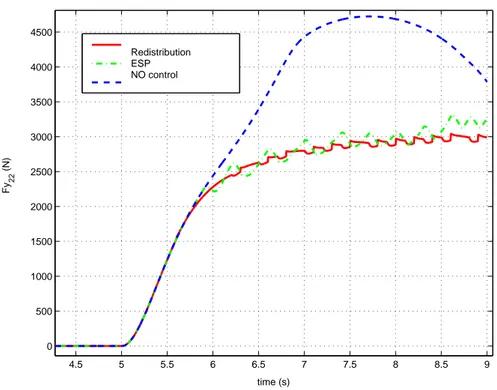
4.5 5 5.5 6 6.5 7 7.5 8 8.5 9 0 500 1000 1500 2000 2500 3000 3500 4000 4500 time (s) Fy 22 (N) Redistribution ESP NO control
vertical load acting on these wheels is null. On the contrary we can observe the side forces transferred by the outer tyres which reach very high values on account of the considerable vertical load and because the slip angles are surely quite wide (the global effect of this set of force is in fact a car which spins around).
With regard to the car provided with the central coupling we can see the effects of the redistribution of torque on the forces. Obviously the longitudinal forces due to the front wheels increase (fig.6.9 and fig.6.10) and contrary the forces transmitted by the rear wheels decrease (fig.6.11 and fig.6.12) when this system is intervening. While the coupling is acting we obtain four tyres which produce longitudinal forces different from zero and both the inner and the outer wheels of the same axle transfer almost the same force (not exactly the same because of the different vertical load which does not allow the inner wheels to exploit the whole drive torque). The global effect is in any case positive to decrease the yaw rate, compared to the situation occurring without using any stability control system. After few seconds only one outer wheel transmitted a significant longitudinal force (fig.6.12), and it causes a positive yaw acceleration. The lateral forces have a more constant value in the previous case, and the effect of the ellipse of grip is clear, in fact when a longitudinal force increases, in the same time the corresponding lateral force decreases (see for example fig.6.9 and fig.6.13). In this way, when we close the valve we decrease the front lateral forces and we increase the rear lateral force, and this fact causes a change in yaw acceleration.
The vehicle which uses the ESP keeps stability exploiting the tyre forces in a different manner. In fig.6.10 and in fig.6.14 we can observe the effects of the brake torque respectively on the longitudinal and lateral force. The longitudinal force reaches significant negative peaks and, being applied on the front outer wheel, it produces a contra-cornering yaw moment. In the same time, when we apply the brake torque the lateral force decreases on account of the tyre behavior in combined slip conditions, and also this fact contributes to avoid oversteer. The performance of the rear inner tyre (fig.6.11 and fig.6.15) is very influenced by the oscillating vertical load and for this reason it presents a not very regular trend both on longitudinal and lateral forces.
In fig.6.17 the yaw acceleration in the three different cases is presented. The graph displays that the non controlled vehicle has a positive yaw acceleration during the whole simulation, hence the yaw rate is continuously increasing. In particular during the last instants the acceleration has a a very high positive slope and it reaches a very high peak.
4 6 8 0 0.1 0.2 0.3 0.4 0.5 time (s)
Yaw accel. (rad/s
2) 5 6 7 8 9 0 0.1 0.2 0.3 0.4 0.5 time (s)
Yaw accel. (rad/s
2) 5 6 7 8 9 −1 −0.8 −0.6 −0.4 −0.2 0 0.2 0.4 0.6 time (s)
Yaw accel. (rad/s
2)
NO control Redistribution ESP
Figure 6.17: Vehicle yaw acceleration in the three different cases
acceleration oscillate around zero, to limit the yaw rate. The redistribution of torque produces a more regular performance than the ESP, in fact the positive and negative peaks remain closer to zero. This fact is positive because, as we can observe in fig.6.3, the bend radius does not deviate from the reference radius as much as using the ESP. However considering that we are transferring the maximum amount of torque allowed by the central coupling it means that using the brake system it is possible to create a much stronger contra-cornering yaw moment.
Now we want to analyze the effects of these systems on the car performance. In all the simulations we used the virtual pedal gas trying to keep constant speed (see par. 3.1.3), and the redistribution of torque system exhibited a good potential also in order to maintain an high velocity. In fig.6.18 we can see that, since the ESP acts on the brake system it obviously makes the vehicle slow down, contrary to the redistribution of torque system, which allows to keep an almost constant speed.
In the end of the simulation the difference between the two speeds of the center of
gravity (VG =
√ u2
+ v2
) is almost 2 m
s, and even if it is not a significant difference for a
normal car, it could be very important for a competition vehicle.
In reference to the vehicle comfort in fig.6.19 we compare the center of gravity
5 5.5 6 6.5 7 7.5 8 8.5 9 45 46 47 48 49 50 51 52 53 54 time (s)
speed (m/s) RedistributionESP
NO control
Figure 6.18: Center of gravity speed
4 4.5 5 5.5 6 6.5 7 7.5 8 8.5 9 −2 −1.5 −1 −0.5 0 0.5 1 time (s) long. acc. (m/s 2) Redistribution ESP
level of longitudinal acceleration the passengers are subjected to. Also in this case we want to remark the negative effect of the strong action of the ESP, which produces a much more variable level of acceleration than the redistribution of torque, with very high positive and negative peaks. For this reason the ESP intervention is surely more annoying and uncomfortable than the “Haldex” coupling action.
6.2
High Speed B
In this simulation we want to illustrate the effects of our stability control system in case the driver tries to impose a trajectory that the car cannot drive along, because of physical reasons, without having a motion with a too wide |β| angle. In this simulation the initial
speed is approximately 74 m
s (corresponding to more than 260
km
h ) and the steer angle
follows a step function with final value equal to 0.5 deg. We present the results obtained providing the vehicle with an Active Yaw Control based on the redistribution of torque. This system proved to be very effective to keep stability in a rear-wheel drive car if any external disturbance is not acting. In this kind of situation in fact a central coupling properly controlled is so good that the vehicle behavior is not improved combining this system with an ESP.
0 100 200 300 400 500 600 700 800 900 −20 0 20 40 60 80 100 120 140 160 180 distance (m) distance (m)
Figure 6.20: Trajectory driven by the car
In fig.6.20 we show the trajectory followed by the vehicle and in fig.6.21 we can analyze the trend of the curve radius.
The average “R” distance is bigger than the reference distance “R” distance (repre-sented in black), but still we achieved a good result. In fact the car does not spin around
5 6 7 8 9 10 11 12 300 400 500 600 700 800 900 time (s) corner radius (m) Figure 6.21: “R” distance 0 2 4 6 8 10 12 −9 −8 −7 −6 −5 −4 −3 −2 −1 0 1 time (s) beta (deg)
Figure 6.22: Body slip angle
Providing the vehicle with the ESP we would not improve the trajectory and the per-formance in terms of comfort and speed would be worse
6.3
External Disturbance
In this simulation we consider a vehicle liable to a lateral force while it is cornering. The initial speed is 35 m
s and the steer angle function is a step with final value equal to 1 deg.
The lateral force is represented in fig.6.23.
0 5 10 15 0 200 400 600 800 1000 1200 1400 1600 time (s) Lateral force (N) Lateral force
Figure 6.23: Lateral force applied from outside
(it is positive, therefore it is directed towards the corner center) and it is applied 0.3 m ahead the center of gravity. Observing the body slip angle in the different conditions we can notice that if we do not intervene the vehicle spins around (fig.6.24).
Providing the car with a central coupling we manage to keep stability, but the body slip angle becomes so wide (it reaches almost -20 deg) that the car motion cannot be considered satisfactory. In contrast to the vehicle supplied just with the redistribution of torque system, acting on the brake system we can improve very much the car behavior. In fact we can maintain the body slip angle within a satisfactory range (it never exceeds -4 deg) and we succeed in bringing the real trajectory closer to the undisturbed trajectory (fig.6.25). This simulation is representative of the higher potential of the ESP, in comparison with our system. The ESP in fact can be more efficacious than an Active Yaw Control based
10 10.5 11 11.5 12 12.5 13 13.5 14 14.5 15 −90 −80 −70 −60 −50 −40 −30 −20 −10 0 10 time (s)
beta angle (deg)
Redistribution NO control ESP
ESP & redistribution
Figure 6.24: Body slip angle
provided by the “Haldex” system. On account of the ellipse of grip the ESP can make the lateral forces decrease more effectively than the redistribution of torque. • It can brake independently each wheel, such a way to exploit the effect of the
longi-tudinal forces (the drive torque causes the same longilongi-tudinal forces on the left and the right wheel, hence they do not produce a significant yaw moment).
However it does not mean that the redistribution of torque is totally useless in this case. We want to remark the fact that combining together the two stability control systems we can bring the trajectory even closer to the undisturbed curve (fig.6.25), and also the ESP intervention changes (fig.6.26).
We want to point out that the applied brake torque is lower combining the ESP with the central coupling. It causes surely an improvement of the vehicle performance and a more comfortable response. In addition it is reasonable to suppose that exploiting the maximum potential of both the systems together we can be able to control more critical situations, in comparison with the conditions we can stabilize using them independently.
305 310 315 320 325 330 335 340 345 350 40 60 80 100 120 140 160 180 200 220 240 distance (m) distance (m) Redistribution NO control ESP
Redistribution & ESP NOT disturbed trajectory
Figure 6.25: Trajectories driven along by the vehicles
10 11 12 13 0 100 200 300 400 500 600 700 time (s) Mb 12 (N*m) 10 11 12 13 14 0 100 200 300 400 500 600 time (s) Mb 12 (N*m) ESP Redistribution & ESP
6.4
Avoidance Manoeuvre
Making this simulation we wanted to check the efficiency of the Active Yaw Control Systems in case the steer angle does not follow a step function, hence the reference yaw rate is continuously variable. Moreover by this simulation we wanted to understand whether to use a control strategy based on steady state references is suitable to control the vehicle during a quick transitory. The steer angle function we used is represented in fig.6.27
0 1 2 3 4 5 6 7 8 9 −0.8 −0.6 −0.4 −0.2 0 0.2 0.4 0.6 time (s)
steering angle (rad)
Steering angle
Figure 6.27: Steer angle function
By means of this input we want to obtain a car which turn first to the right then to the left, as if the driver wanted to avoid an obstacle. The initial car speed is 60 m
s.
In fig.6.28 we notice an important improvement of vehicle behavior using the stability systems.
Without using any kind of control the vehicle moves almost 12 m away from the initial straight before approaching again the initial trajectory. Using just the central coupling this distance reduces to less than 8 m. The ESP system can bring the vehicle even closer. Obviously the lower is this distance, the safer is the manoeuvre, in fact a normal road is not very wide and for example a car which drives 12 m on the right can easily crash against an obstacle placed on the side. Also in this simulation the ESP allows to have a better
300 350 400 450 500 550 −12 −10 −8 −6 −4 −2 0 2 4 6 distance (m) distance (m) NO control Redistribution Redistribution & ESP ESP
Figure 6.28: Trajectories followed by the vehicle
performance than the “Redistribution of Torque”. It occurs on account of the two reasons mentioned in par.6.3 and because
• Using the “Haldex” coupling we cannot obtain (in a rear-wheel drive car) an effect similar to a brake torque applied on the rear wheels. As shown in fig.6.29 and fig.6.30 both the rear brakes are activated by the ESP to execute the manoeuvre.
It is very interesting to realize that also in this case to combine the effects of the ESP and of the “Haldex” system improves the performance of the Active Yaw Control System, making the car drive along a narrower corner. Moreover, even if during an emergency manoeuvre it is not very important, combining the two systems we improve also in this case the car performance and the vehicle comfort. In fact, for example in fig.6.29, we can notice that the ESP activates the rear left brake much less time if it is combined with a proper redistribution of torque strategy.
5 6 7 8 9 0 100 200 300 400 500 600 700 time (s) Mb 21 (N*m) 5 6 7 8 9 0 100 200 300 400 500 600 700 time (s) Mb 21 (N*m) Redistribution
& ESP ESP
Figure 6.29: Brake torque applied to the rear left wheel depending on the activated stability control systems 5 6 7 8 9 0 50 100 150 200 250 300 350 400 450 500 time (s) Mb 22 (N*m) 5 6 7 8 9 0 50 100 150 200 250 300 350 400 450 500 time (s) Mb 22 (N*m)
Redistribution & ESP ESP
Figure 6.30: Brake torque applied to the rear right wheel depending on the activated stability control systems