UNIVERSIT`
A DI PISA
Laurea Magistrale in Ingegneria
Robotica e dell’Automazione
Tesi di Laurea
Control architecture for natural motion
in soft robots
Candidato:
Cosimo Della Santina
Relatore:
Prof. Antonio Bicchi
Correlatore:
Prof. Carlo Alberto Avizzano
Abstract
In soft robots fixed (SEA) or physically adjustable (VSA) compliant elements are delib-erately introduced in the robot structure, to obtain human-like behavior in terms of smooth movements, shock absorption, safety and performance improvements.
The human high performance relies not only on the muscular-scheletric “design”, but also on its effective control the central and peripheral nervous system (CNS and PNS respectively). On the other hand automatic control theory requires substantial advancements to achieve ac-ceptable performance in spite of the complexity of the nonlinear hard-to-model soft robots dynamics.
The majority of existing control approaches for soft robots have the strong drawback of requiring an accurate model identification process, that is hard to be accomplished and time consuming. Model-free algorithms are promising but still confined to specific tasks, such as the induction of stable cyclic motions or the damping control to suppress undesirable oscillations.
The aim of this work is to design a model-free control system that ensures natural move-ments in soft robots. Due to the similitudes between muscular-scheletric system and soft robots, we decided to develop a controller that can replicate some functionalities of the central ner-vous system: learning by repetition, after-effect on known and unknown trajectories and state covariation in tasks execution.
The control architecture is organized on two levels. The lower level of control performs dynamic inversion (i.e. it estimates a map that given the desired state space evolution, returns the necessary input) allowing to capitalize information coming from standard iterative learning control techniques. The algorithm relies on a parametrization of the sub-space of the state evolutions, and on a discretization of the control space. The higher level of control deals with task execution, performing degree of freedom redundancy management through a model--predictive-control-like method. Finally an algorithm for high and low level merging in order to achieve task specific dynamic inversion is proposed. Simulations and experiments were performed on VSA with antagonistic mechanism (qbmoves), to show the effectiveness of the proposed control system.
1
Introduction
Human performance makes the difference in real life tasks. Some examples are: open breaches in walls and roofs (high peak power), sustain hours of operations (high efficiency), work in dangerous scenarios (high robustness).
These tasks are achieved by the human body also thanks to its compliance, that can be modified through co-contraction of agonist-antagonist muscles, allowing for soft and strong operations. Hence in the last years the idea of realize robots with analogous mechanical chara-teristics came out in the scientific community.
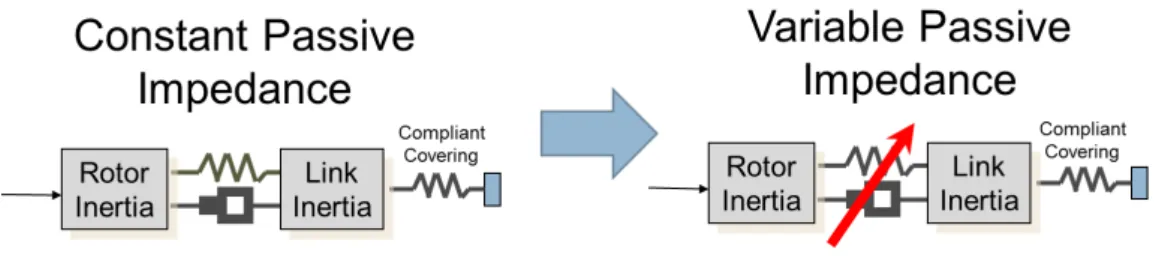
Soft robots [1] are robotic systems designed to obtain human-like behavior in terms of smooth movements, shock absorption, safety and performance improvements. These robots are actuated by compliant mechanisms. Historically the first one of these actuators was the serial elastic actuator (SEA), with passive fixed impedence. An important evolution was the introduction of actuators with variable impedence (stiffness, damping), see figure 1. Many mechanical architures exists [22], and tipically they present complex, nonlinear, hard-to-model dynamics.
Examples are cCub [21], which has passive compliance in the major joints of the legs, and VPDA [9], a semi-active friction based variable physical damping actuator unit, both developed at the IIT; the DLR hand-arm system [8], comprises three different types of VSA, respectively in the arm, in the wrist, and in the hand; the VSA-CubeBot [4], developed at the Piaggio Center, are modular-servo VSA multi-unit systems, that implements an agonist-antagonist mechanism. VSA-CubeBot is used in this work as test-bed for proposed algorithm.
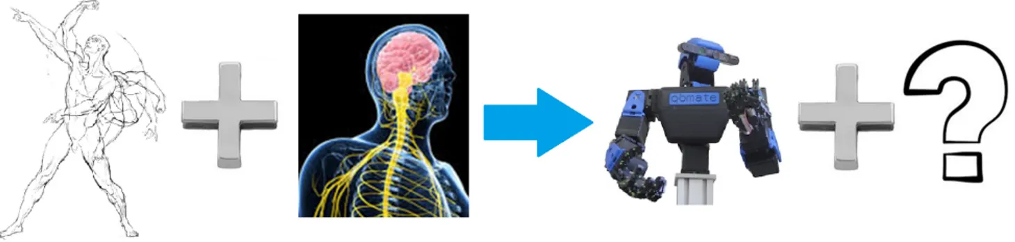
The human muscles can achieve the described performances also thanks to the effective synergistic union between the muscular-scheletric system and the brain. Due to the described criticalities, soft robots have not a so effective “brain” (figure 2).
The majority of existing model-based control approaches for soft robots, has the strong drawback of requiring an accurate model identification process, that is hard to be accomplished and time consuming. In [15] feedback linearization of VSA is faced. In [7] is addressed the problem of choose the inputs for maximizing the velocity of a link at a given final position. In [3] a framework for simultaneous optimisation of torque and stiffness, incorporating real-world constraints is proposed.
On the other hand model-free algorithms are promising but still confined to specific tasks, as for example induction [10] or damping [16] of oscillations.
Figure 1: Technologies evolution.
The purpose of this work is to design a model-free algorithm capable to control an uncertain Lagrangian system, such as a soft robot. The idea underlying this work is to take inspiration from how the central nervous system (hereinafter CNS) manages the human body system according to the state of the art motor control theories.
Mark Latash, a motor control scientist, defines motor control as: “[Motor Control] can be defined as an area of science exploring how the nervous system interacts with the rest of the
Figure 2: Muscular-scheletric system has the brain that control it. Which system control a soft robot?
body and the environment in order to produce purposeful, coordinated movements” [12] Two problems faced by CNS are:
• Unknown nonlinear dynamic: human body is a complex system, with strong nonlinearities at every level.
• Degree of freedom (hereinafter DoF) redundancy problem. Three types of redundancy are typically identified:
– Anatomical: Human body is characterized by a complex highly redundant struc-ture. The number of joints is greater than the number DoFs necessary to accomplish a generic task, and the number of muscles is greater than the number of joints. – Kinematic: Infinite joints trajectories can achieve the same task, or simply perform
the same end effector point to point movement.
– Neurophysiological: The muscle consists of hundreds of motor units, and they are activated by moto-neurons that can spike with different frequency (hundreds of variables).
2
From Motor Control To Motion Control
Soft robots present analogous problems:
• Unknown nonlinear dynamic: It is well-known that robotic systems are nonlinear and it was already discussed how the soft actuators have a hard-to-model non linear dynamic. Moreover variable stiffness antagonistic actuators present dynamic behavior similar to human muscles (same equilibrium point and stiffness).
• DoF problem: Soft robots present both anatomical (they tipically have more than one motor per joint) and kinematic redundancy.
Hence a way to solve the problem of soft robot control could be to get information about the way CNS manages the body.
Understand how CNS works is an open problem yet, and no univocal theory exists (e.g. internal model vs. equilibrium point). Rather than trying to replicate a not yet well under-stood structure, in this work we discuss how to replicate the CNS functionalities, where largely accepted objective data exist.
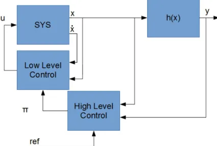
• Low Level(hereinafter LL): to perform dynamic inversion.
• High Level(hereinafter HL): to perform DoFs abundance management.
Figure 3: Control structure. u is the low level control variable, π is the high level control variable, ref is the reference in the task space, x is the position vector, y is the output vector, h(·) is the output function.
2.1
Low Level Control
The purpose of this level is to perform dynamic inversion of the dynamical system. CNS presents three peculiar characteristics in learning new movements that we are interested to reproduce:
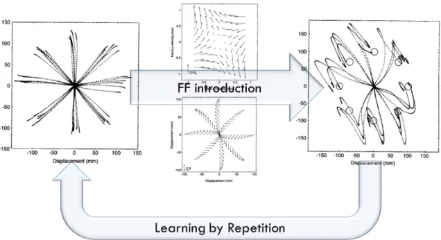
(i) Learning by repetition: CNS inverts an unknown dynamic over a trajectory, repeating it several times. Figure 4 represents a classical experiment. The subject is asked to reach some points. Then a force field is introduced. Initially trajectories are strongly deformed. After repetitions of the same tasks, performances obtained before the introduction of the force field are achieved again.
(ii) Aftereffect over a learned trajectory: By removing the force field, subjects present de-formations of the trajectory specular to the initial deformation due to the force field introduction. This behavior is called mirror-image aftereffect (figure 5a).
(iii) Aftereffect over trajectories not learned: by removing the force field, subjects exhibit deformations of the trajectories both in the learned trajectory and in a new one (figure 5b).
Internal model theory claims that neural processes that simulate the response of the motor system exist. Internal models are able to explain all the three aspects previously mentioned [24]. The CNS is considered able to regress these models from experience, including in them also external disturbances (e.g. a force field).
From a robotics point of view, in [18, 14] the control of robot through complete model estimation is reviewed. Gaussian Process Regression (GPR) is shown to be the only sufficiently
Figure 4: Representation of a typical experiment demonstrating learning by repetition human capa-bilities.
Figure 5: (a) Aftereffect is present removing the force field (obtained in this experiment by a rotating platform). (b) Aftereffect is present also in unknown trajectories.
accurate method to be used for control purposes. Despite this, GPR is considered practically inapplicable due to its computational cost (O(n3) with respect to the number of regression points).
Therefore, we follow another way in this work. Learning by repetition is naturally inter-pretable in terms of Iterative Learning Control (ILC). An intuitive definition is given in [13]: “The main idea behind ILC is to iteratively find an input sequence such that the output of the system is as close as possible to a desired output. Although ILC is directly associated with control, it is important to note that the end result is that the system has been inverted”.
ILC exploits the whole previous iteration error evolution to update a feedforward command, according to the law: ui+1= ui+ re(t, i), where the function re(t, i) identifies the ILC algorithm
and ui is the control action at the i − th iteration. In this work we use an Arimoto low [20] re(t, i) = ILCP ID(t, i) + P ID(t, i + 1), where P ID(t, i + 1) is a proportional, integrative
and derivative feedback, and ILCP ID(t, i) is a pure feedforward proportional, integrative and
derivative updating. In the thesis we derive a simple convergence condition for Lagrangian systems.
Simulations are done on a RR arm (each link has a weight of half kg and is half meter long). Viscose friction and gravitational field are added as uncertainties. The algorithm reduces the mean trajectory tracking error of one order of magnitude in about 10 steps, and of two order of magnitude in about 50 steps. The graph will be shown in the presentation, many other simulations are provided in the whole thesis.
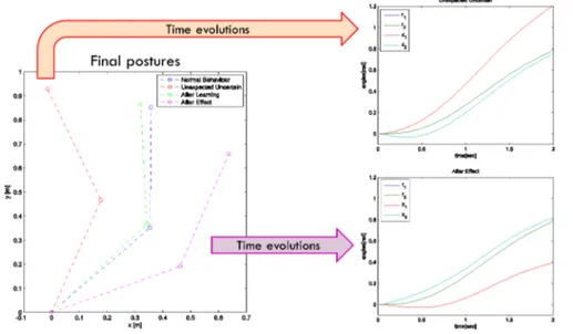
As summarized in figure 6, ILC is able to explain aftereffect over experienced trajectories.
Figure 6: ILC is able to explain after effect over experienced trajectories. The system is trained to follow the reference evolution shown in the graphics on the right. The associated final posture is the blue one. Then a force field is introduced, and the trajectory is deformed reaching the red posture (time evolution is in the upper right). Learning is performed and the system is again able to reach a final position near the blue one. Finally the field is removed, and the arm presents a final posture (the purple one) and a time evolution (the lower right) specular to the red ones.
ILC is a local method and cannot explain aftereffect over unknown trajectories. Information obtained during learning needs to be capitalized in some way. Existing methods contemplate the independent estimation of a complete model of the system (e.g. [17], [2]). The limitations of complete model estimation approach are already explained in previous pages: a novel method combining generalization, accuracy and acceptable computational costs is needed.
Defining I : C0([0, tf in)) → C0([0, tf in)) as the system inverse functional (considering tf in
the terminal time of the evolutions), it is possible to assert that ILC execution returns a couple < ¯x, I(¯x) >, with ¯x desired evolution. Therefore the idea is to use a regression technique in order to estimate I from the set of < ¯x, I(¯x) > already learned. The problem is that making a regression of a functional is a really complex task.
Therefore functional is transformed into a function. Let’s define: • a parameterization of a subspace P ⊆ C0([0, t
f in)) of dimension p, B : Rp → P .
• a time discretization of d steps, S : C0([0, t
f in)) → Rd
The parameterization constrains the low level controller to manage only a sub-set of the possible evolutions.
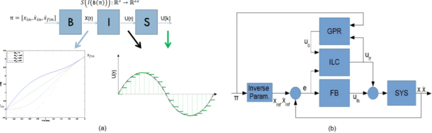
The the map we are interested to is S(I(B(π))) : Rp → Rd(figure 7a). π refers to parameters
array.
Figure 7: (a) S(I(B(π))) function graphical representation: B(·) is the parameterization function, I(·) the system inverse functional, S(·) is the time discretization. (b) Low Level control scheme: u = uf b+ uf f is the low level control variable, u0 is the a-priori feedforward estimation returned by
the map (GPR), π is the high level control variable, x is the configuration vector. The block FB represents the feedback controller, ILC represents the ILC algorithm, GPR represents the regressed map, the block Iverse Param. implements the B(·) function.
The choice of the sub-space P can be arbitrary. Previous works (e.g. [6, 5, 23]) show that many human movements minimize the jerk (derivative of acceleration) and that trajectories that minimize jerk are 5-th order polynomial splines. For practical purposes a smaller subspace is chosen: 5-th order monic polynomial with two constraints, which reduce space dimension to 3 and ensure that subspace elements juxtaposition is C2, are adopted: ∂
2x
∂2tt={0,t
f in}
= 0 and xf in = xin+ ˙xf intf in. Where xin and xf in are respectively the initial and final values of
the polynomials. Following this choice π = [xin, ˙xin, ˙xf in]. In figure 7a some evolutions are
presented in this sub-space at varying of ˙xin.
The regressed map is used for new trajectories estimation. The remaining errors can be corrected with further iterations of ILC algorithm. The new result of ILC is then used for map regression (figure 7b). GPR is used as regression algorithm.
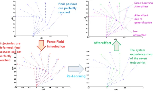
In figure 8 we summarize simulations (RR arm, controller, and force field as previously described) that show that the proposed regression techniques present aftereffect over unknown trajectories (behavior (iii)).
Figure 8: Proposed regression technique explain aftereffect over unknown trajectories.
For performance evaluation, 104 simulation of random tasks for a RR manipulator in the subspace are performed, with and without a map learned with 32 limit cases. The mean error with the map is 0.0596 rad sec with a variance of 0.0013 rad2sec2. The mean error without the
map is 0.5644 rad sec with a variance of 0.1137 rad2sec2.
ILC was tested on an RR qbmoves VSA arm. ILC presents good performances at various values of stiffness. Moreover it presents the described capability of adapting to dynamical uncertainties. The regression mechanisms has really good performances reducing the error of trajectories of about the 80% (videos will be shown in the presentation).
2.2
High Level Control
Low level controller abstracts the largely unknown and nonlinear system into a discrete one with a known dynamics that depends on the chosen subspace (figure 9b). The high level control variables are the base parameters: π = [xin, ˙xin, ˙xf in] (figure 9a). The role of the High
Level Controller is to choose the sequence of πk[3], the third element of πk, because the first
two elements are constrained by the initial conditions. The obtained high level dynamic is xk+1 = xk+ tf inπ
[3] k ;
It is supposed that higher level of control specifies a task to be accomplished. A task will be defined as a cost function and a set of constraints.
The High Level Control is defined by an optimization problem and by an algorithm that solve it. Optimization problem can be formulated as:
min∆π,xkh(x) − ¯ykQ+ k∆πkR kδx(x)k ≤ xlimit kδπ(∆π)k ≤ ∆πlimit xk+1 = xk+ tf inπ [3] k
Where h(x) selects variables of interest for the task, ∆π refers to the difference between two consecutive control commands (actuation cost), δx(x) and δπ(π) are generic constraint
Figure 9: (a) Example of global evolution in blue, with slope pointed out in green (b) Architecture with system abstracted by the low level controller into a known discrete system D plus an uncertain φ due to imperfect inversion. π is the high level control variable, ref is the reference in the task space, x is the configuration vector, y is the output vector, h(·) is the output function.
functions. Bold case represents a vector containing the whole temporal sequence of values (e.g. x= [x. 1, x2, ...]).
This resolution of redundancy is much more general compared to classical pseudo-inversion techniques. It permits to consider: nonlinear hard constraints, actuation costs, general cost functions (e.g. being in a point at a certain time).
Two algorithm that can be used to solve the problem are: pre-solving the problem and controlling the system over xoptthrough a proportional (P) controller (dead beat); recalculating
the optimum on-line: model predictive control (MPC) approach.
The quality of the task execution is strongly affected by the accuracy of the learned low level map (figure 10).
Figure 10: An RR arm is controlled with pre-solving technique (one joint evolution): (a) Rough map with high tracking error, (b) Fine map with Low tracking error.
The possible approaches are: to pre-learn the map as we have done in the previous section, to design an algorithm that merges the high and low level controllers.
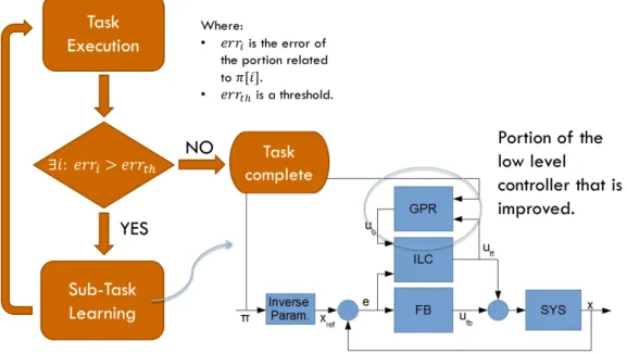
Here we choose the second approach. If a new task is not properly executed then the accuracy of the map should be improved. The resulting algorithm is described in figure 11.
With this algorithm the Low Level map is learned in a task-oriented way: most of the points will be collected in the portions of the subspace that are more used in the tasks, obtaining a very good trade-off between map dimension and accuracy.
A numerical example is performed. Example description: Execution of 20 tasks itera-tively; the task consists in moving the arm such that kh(x) − ¯yjk is minimized, where h(x) =
Figure 11: Merged algorithm block diagram.
0.5cos(x1) + 0.5cos(x1 + x2) and ¯yj is the desired evolution of task j; Joints limits are
consid-ered; No initial map is present; the system controlled is a numerical model of a variable stiffnes qbmoves RR arm.
Using merged algorithm, map converges to a complete representation of the inverse system (no more learning is needed) after ∼ 12 tasks, with both solution algorithms (figure 13).
MPC approach presents better performances because re-optimization at each iteration per-mits to fully exploit the task redundancies (figure 13). E.g. if the system moves on ˜x different from the desired one ˆx, but such that h(˜x) = h(ˆx), P controller corrects the “error”, MPC not. Conventionaly MPC is hardly applicable to mechanical systems due to their high band-widths, but this architecture allows MPC application requiring its execution every tf in only.
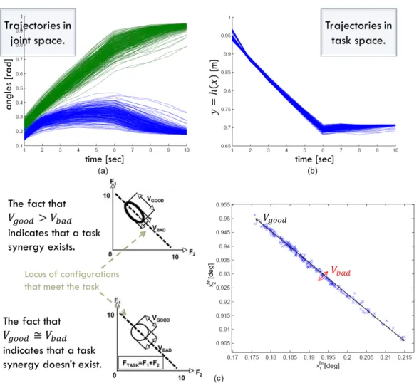
The modern definition of synergy, given in [11], is: “[...] a hypothetical neural mecha-nism that ensures task-specific co-variation of elemental variables providing for desired stability properties of an important output (performance) variable” Let h(x) be the “important out-put variable”, according to this definition the high level control we are talking about presents Vgood >> Vbad in the configuration space, showing a Synergy - like behavior (figure 12), where
Vgood is the variance through the directions where h(·) is constant and the constraints are
verified, and Vbad is the variance in the other directions [19].
3
Conclusions
In this work a new algorithm that allows to control uncertain Lagrangian systems was developed. The algorithm ensures some characteristics of human natural movement: Learning by repetition, aftereffect in known and unknown trajectories, capability of ensuring task specific co-variation (synergy-like behavior). Simulations and experiments were done also on qbmoves VSA in order to evaluate performances and MC similitudes.
Figure 12: The task, executed many times (same output reference) with small variations in the initial conditions, shows a high variability in joints evolutions (a), maintaining task performances (b). In (c) final configurations are summarized in the same plane, allowing to visualize the synergy-like behavior of the high level controller.
References
[1] Alin Albu-Schaffer, Oliver Eiberger, Markus Grebenstein, Sami Haddadin, Christian Ott, Thomas Wimbock, Sebastian Wolf, and Gerd Hirzinger. Soft robotics. Robotics & Au-tomation Magazine, IEEE, 15(3):20–30, 2008.
[2] Muhammad Arif, Tadashi Ishihara, and Hikaru Inooka. Incorporation of experience in iterative learning controllers using locally weighted learning. Automatica, 37(6):881–888, 2001.
[3] David J Braun, Florian Petit, Felix Huber, Sami Haddadin, P Van Der Smagt, A Albu-Schaffer, and Sethu Vijayakumar. Optimal torque and stiffness control in compliantly actuated robots. In Intelligent Robots and Systems (IROS), 2012 IEEE/RSJ International Conference on, pages 2801–2808. IEEE, 2012.
[4] Manuel G Catalano, Giorgio Grioli, Manolo Garabini, Fabio Bonomo, M Mancinit, Niko-laos Tsagarakis, and Antonio Bicchi. Vsa-cubebot: A modular variable stiffness platform for multiple degrees of freedom robots. In Robotics and Automation (ICRA), 2011 IEEE International Conference on, pages 5090–5095. IEEE, 2011.
[5] Tamar Flash and Neville Hogan. The coordination of arm movements: an experimentally confirmed mathematical model. The journal of Neuroscience, 5(7):1688–1703, 1985.
[6] Jason Friedman and Tamar Flash. Trajectory of the index finger during grasping. Exper-imental brain research, 196(4):497–509, 2009.
[7] Manolo Garabini, Andrea Passaglia, Felipe Belo, Paolo Salaris, and Antonio Bicchi. Opti-mality principles in variable stiffness control: The vsa hammer. In Intelligent Robots and Systems (IROS), 2011 IEEE/RSJ International Conference on, pages 3770–3775. IEEE, 2011.
[8] Markus Grebenstein, Alin Albu-Scha?ffer, Thomas Bahls, Maxime Chalon, Oliver Eiberger, Werner Friedl, Robin Gruber, Sami Haddadin, Ulrich Hagn, Robert Haslinger, et al. The dlr hand arm system. In Robotics and Automation (ICRA), 2011 IEEE Inter-national Conference on, pages 3175–3182. IEEE, 2011.
[9] Matteo Laffranchi, Nikolaos G Tsagarakis, and Darwin G Caldwell. A variable physi-cal damping actuator (vpda) for compliant robotic joints. In Robotics and Automation (ICRA), 2010 IEEE International Conference on, pages 1668–1674. IEEE, 2010.
[10] Dominic Lakatos, Florian Petit, and Alin Albu-Schaffer. Nonlinear oscillations for cyclic movements in variable impedance actuated robotic arms. In Robotics and Automation (ICRA), 2013 IEEE International Conference on, pages 508–515. IEEE, 2013.
[11] Mark L Latash. Motor synergies and the equilibrium-point hypothesis. Motor control, 14(3):294, 2010.
[12] Mark L Latash. Fundamentals of motor control. Academic Press, 2012.
[13] Ola Markusson, H˚akan Hjalmarsson, and Makael Norrlof. Iterative learning control of nonlinear non-minimum phase systems and its application to system and model inversion. In Decision and Control, 2001. Proceedings of the 40th IEEE Conference on, volume 5, pages 4481–4482. IEEE, 2001.
[14] Duy Nguyen-Tuong, Jan Peters, Matthias Seeger, and Bernhard Sch¨olkopf. Learning in-verse dynamics: a comparison. 2008.
[15] Gianluca Palli, Claudio Melchiorri, and Alessandro De Luca. On the feedback linearization of robots with variable joint stiffness. In Robotics and Automation, 2008. ICRA 2008. IEEE International Conference on, pages 1753–1759. IEEE, 2008.
[16] Ott C. Petit, F. and A. Albu-Schaffer. A model-free approach to vibration suppression for intrinsically elastic robots. In Robotics and Automation (ICRA), 2014 IEEE International Conference on, 2014.
[17] Oliver Purwin and Raffaello D’Andrea. Performing aggressive maneuvers using iterative learning control. In Robotics and Automation, 2009. ICRA’09. IEEE International Con-ference on, pages 1731–1736. IEEE, 2009.
[18] Stefan Schaal and C Atkeson. Learning control in robotics. Robotics & Automation Mag-azine, IEEE, 17(2):20–29, 2010.
[19] John P Scholz and Gregor Sch¨oner. The uncontrolled manifold concept: identifying control variables for a functional task. Experimental brain research, 126(3):289–306, 1999.
[20] Jianxia Shou, Daoying Pi, and Wenhai Wang. Sufficient conditions for the convergence of open-closed-loop pid-type iterative learning control for nonlinear time-varying systems. In Systems, Man and Cybernetics, 2003. IEEE International Conference on, volume 3, pages 2557–2562. IEEE, 2003.
[21] Nikolaos G Tsagarakis, Zhibin Li, Jody Saglia, and Darwin G Caldwell. The design of the lower body of the compliant humanoid robot ?ccub? In Robotics and Automation (ICRA), 2011 IEEE International Conference on, pages 2035–2040. IEEE, 2011.
[22] Bram Vanderborght, Alin Albu-Sch¨affer, Antonio Bicchi, Etienne Burdet, Darwin G Cald-well, Raffaella Carloni, M Catalano, Oliver Eiberger, Werner Friedl, Ganesh Ganesh, et al. Variable impedance actuators: A review. Robotics and Autonomous Systems, 61(12):1601– 1614, 2013.
[23] John Wann, Ian Nimmo-Smith, and Alan M Wing. Relation between velocity and curvature in movement: equivalence and divergence between a power law and a minimum-jerk model. Journal of Experimental Psychology: Human Perception and Performance, 14(4):622, 1988.
[24] Daniel M Wolpert, R Chris Miall, and Mitsuo Kawato. Internal models in the cerebellum. Trends in cognitive sciences, 2(9):338–347, 1998.