3 – GEOLOGICAL-HYDROGEOLOGICAL-GEOCHEMICAL STUDY OF MOUNTAIN AQUIFER SYSTEMS

3 – GEOLOGICAL-HYDROGEOLOGICAL-GEOCHEMICAL

STUDY OF MOUNTAIN AQUIFER SYSTEMS

The main water resources present in the mountain area are karst aquifers hosted in metamorphic and non-metamorphic limestone. Secondary aquifers are present in noncarbonate fractured rocks and in porous surface debris cover. All of these systems were already the subject of numerous studies and researches (ORSINI, 1987; FORTI et al.,

1990; DOVERI, 2000; CIVITA et al., 1991; PICCINI et al., 1999; MUSSI et al., 1998; FST,

2002; DOVERI et al., 2005; FST, 2005), but the considerable amount of information

collected needs to be interpreted in an organic and systematic way, using a multidisciplinary geological, hydrogeological and geochemical-isotopic approach.

This investigation, aimed at assessing the aquifer systems of the study area, comprises a first stage of sampling followed by a second phase of chemical and isotopic analyses (section 3.1). In particular, during the first phase, main springs hosted in carbonate rocks, “secondary” springs, some samples of rainwater, atmospheric particulate matter (PM10) and carbonate rocks hosting the main aquifers were sampled. Sampling of all these different geo-environmental matrices is a must for the proper investigation of water-rock interaction processes.

The concentration of major components (Ca, Mg, Na, K, Cl, SO4, NO3 and SiO2), selected trace components (B, F, Fe, Mn, Cr, Cu, Ni, Pb and Zn) and some stable isotope ratios (2_H/1_{H and} 18_O/16_{O of H}

2O and 13C/12C of Total Dissolved Inorganic Carbon, TDIC) were determined on collected samples. Sampling and analytical methods are described in details in the next sections.

Processing and interpretation of obtained results followed three main phases:

- A phase in which water-rock interaction was modelled and elementary fluxes arising from this process were evaluated (section 3.2). In particular, the possible dissolution of atmospheric particulate matter (PM10) in rainwater was assessed and the interaction between rainwater and carbonate rocks was modelled, using the EQ3/6 software package and adopting the double solid reactant approach (ACCORNERO & MARINI,

2008; LELLI et al. 2008) to reconstruct the rock-to-water release of trace components and

their fate in the aqueous solution.

- A phase aimed at defining the recharge areas of main hydrogeological systems present in the area of interest through a multidisciplinary approach based on chemical and isotopic data, in close synergy with purely geological and hydrogeological considerations.

- A phase of synthesis of all the available information, aimed at reconstructing the geological-hydrogeological-geochemical conceptual model of the study area.

3.1 – SAMPLING, CHEMICAL AND ISOTOPIC ANALYSES

In any geo-environmental investigation, the sampling phase is one of the most critical activities, in that adequate collection of samples, which must be representative of each matrix of interest, is an essential prerequisite. In contrast, erroneous sampling can lead to bad results in the subsequent stages of data analysis and processing-interpretation. For the same reason, the analytical work has to be carried out in a proper way as analytical data of high quality are needed for a correct understanding of active processes.

3.1.1 – Sampling, chemical and isotopic analyses of rocks

Ten rocks samples and two samples of active stream sediments (figure 3.1) were collected for the characterization of the lithologies hosting the major aquifers in the study area. The two active stream sediments were collected at the emergence of Mount Carchio springs (sample S1) and at the outlet of Ponte Stazzemese 2 spring (sample S2; photo 3.1).

Collected samples were characterized through Scanning Electron Microscopy analysis, chemical analysis of major and trace elements (Table I.Ia in Appendix I), X-Ray Diffractometry (XRD) and determination of the 13_C/12_{C isotopic ratio (Table I.Ib in} Appendix I).

Figure 3.1 – Location of rock samples and stream sediment samples

3.1.2 – Sampling, chemical and isotopic analyses of PM10 and rainwater

For the characterization of the atmospheric particulate matter three monitoring stations (photo 3.2) were used.

They were installed in three distinct sites at different altitudes (figure 3.2). Together with PM10 some rainwater samples were also collected.

The stations consist of an environmental air sampling system for PM10 including a filter holder assembly and a constant-flow controller.

Cellulose nitrate membrane filters with a porosity of 0.45 μm were utilized to collect the atmospheric particulate matter. Gauss-Boaga coordinates and altitude of the three monitoring stations and sampling times for each collected filter are reported in table 3.1.

Photo 3.2 – Particulate matter station

Figure 3.2 – Location of PM10 and rainwater sampling stations

Table 3.1. Locations and altitude of the monitoring stations, and sampling times for each collected filter

Sample code Location Start Stop X (m) Y (m) Altitude _{(m asl)} PM1_22/01 Carchio 22/01/2010 10.30 25/01/2010 9.55 1595964 4876209 847 PM2_22/01 Corchia 22/01/2010 14.30 25/01/2010 11.20 1604177 4875563 824 PM3_23/01 Matanna 23/01/2010 11.30 27/01/2010 10.30 1606200 4872495 714 PM1_25/01 Carchio 25/01/2010 9.55 27/01/2010 13.30 1595964 4876209 847 PM2_25/01 Corchia 25/01/2010 11.20 27/01/2010 1604177 4875563 824 PM3_27/01 Matanna 27/01/2010 10.30 01/02/2010 9.00 1606200 4872495 714 PM1_27/01 Carchio 27/01/2010 13.30 02/02/2010 13.00 1595964 4876209 847

Atmospheric particulate matter collected on filters was characterized through SEM-EDS analyses, while the rainwater samples were analyzed for the contents of major dissolved constituents (HCO3, Cl, SO4, NO3, Ca, Mg, Na, K) and the 18O/16O and 2H/H isotopic ratios of H2O.

3.1.3 – Sampling, chemical and isotopic analyses of waters

A total of 49 water samples were collected during three distinct campaigns: 19 on May 2009, 23 on September 2009 and 7 on July 2010. The first two campaigns were aimed at characterizing, chemically and isotopically, both the main karst hydrogeological systems and the small and shallow circuits in two different times of the year, roughly corresponding with the end and beginning of the rainy period, generally extending from September to May. In July 2010 only the major karst springs and some new springs (not investigated in previous campaigns) were sampled. The location of sampling points is given in the simplified geological map of Figure 3.3.

Collected springs are located at altitudes ranging from a minimum of 10 m asl (Porta Springs PR1, PR2 and PR3) and a maximum of 850 and 870 m of the “Alpe della Grotta” spring (RF), near the “Forte dei Marmi” mountain hostel, and the Moscoso spring (MS), respectively. Other springs have altitudes of 300 to 600 m asl.

The following field measurements were carried out at each sampling site (table I.IIa, Appendix I):

- temperature, by means of a digital thermometer;

- pH by means of a portable, digital mV-pH-meter equipped with a glass electrode and a probe for temperature compensation; two pH buffers, with nominal pH values of 4.01 (HI 7004) and 7.01 (HI 7007) at 25°C, were used for pH calibration at each sampling site;

- Eh by means of a portable, digital mV-pH-meter (0.1 mV sensitivity; scale ±1400 mV) equipped with a Pt electrode (see different configurations) and automatic temperature compensator; the performance of the redox instrument was tested against the ZoBell’s solution, consisting of a 0.1 molal KCl solution containing equimolal amounts of K4Fe(CN)6 and K3Fe(CN)6;

- conductivity by means of a portable, digitable conductivity-meter equipped with a suitable cell (range 0.1-100,000 μS/cm); the instrument was calibrated using suitable standard solutions, whose conductivity encompasses the range of the natural waters of interest;

- total alkalinity by acidimetric titration using HCl 0.1 N and methyl orange as indicator, using a microdosimeter (minimum added HCl volume 0.5 μL) which allows one to work with 200-1000 μL of water;

- flowrate (if possible), measuring either the time needed by a leaf or some other floating object to travel a known distance along the flow channel or the time needed to fill a container of known volume.

For each sampling the following aliquots were taken:

‐ 1 raw aliquot (TQ) in 125 ml polyethylene (PE) bottles for the determination of anions.

‐ 1 TQ in 50 ml PE bottles for the determination of the 2H/1H e 18O/16O isotopic ratio of water.

‐ 1 Filtrated and Acidified (filtered through membranes with pore size of 0.45 μm and acidified through addition of HNO3, Merck Suprapur or equivalent) in 50 ml PE bottle (pre-washed with HCl) for the determination of cations, silica and trace metals.

‐ 1 TQ in 500 ml PE bottle for the determination of the 13C/12C isotopic ratio of total dissolved inorganic carbon (TDIC).

Chemical analyses were performed at the laboratories of the Institute of Geosciences and Earth Resources (IGG) of CNR in Pisa using the following techniques:

• Ion chromatography for the determination of chloride, nitrate and sulphate; • UV-VIS spectrophotometry for the determination of silica after the development of the silico-molybdic complex, yellow oxidized form;

• Atomic Absorption Spectrometry for the determination of calcium, magnesium, sodium and potassium;

• ICP-AES for the determination of trace constituents: arsenic, chromium, copper, iron, manganese, nickel, lead, zinc and boron.

• ion-selective electrode potentiometry for the measurement of fluoride.

Results of chemical analyses are reported both in weight units in the tables I.IIb and I.IId (Appendix I) and in equivalent units in the Table I.IIc (Appendix I), to perform the ionic balance calculations for each spring. In fact, for the principle of electroneutrality of the aqueous solution, the sum of anions (Σanions) must be equal to that of cations (Σcations) if the concentrations are expressed in equivalent units. In other terms, the ion budget, that is the difference Σcations-Σanions, should be zero. In practice, there is always a certain ionic unbalance, due to different types of errors, which is calculated using the following formula: 100 ⋅ + − = anions cations anions cations % unbalance _ ion Σ Σ Σ Σ

Usually the analysis is considered of acceptable quality if the calculated ion unbalance is within the range ± 3%.

All the springs sampled in May 2009 and most of those surveyed in September 2009 have ion unbalance within the range ± 3%, apart from Bendiloni/09 and Marginetta/09, whose ion unbalance is around 4%, and Pancetto/09, with 8.8% unbalance despite its analysis was repeated several times (table 2.4). The chemical analyses for these three springs are considered, however, acceptable because for waters of very low conductivity, as in this case (less than 100 µS/cm), the limit of acceptability may be extended up to ± 10%.

It should be emphasized that the calculation of ion unbalance does not provide any indication on the quality of analytical data for minor and trace constituents.

Isotopic analyses (δ18_{O, δ}2_{H e δ}13_{C) were made at the Stable Isotope Unit, National} Centre for Scientific Research “Demokritos”, Athens, Greece with a Thermo Scientific Delta V Plus mass spectrometer (GasBench II device). Stable Isotope Unit is accredited

(EPSTEIN & MAYEDA, 1953). The δ2H value of water was determined through analysis of

gaseous H2 generated by the Platinum catalyst method. For the analysis of the δ13C value of TDIC, BaCO3 was precipitated and reacted with ortho-phosphoric acid (99%) at 72°C, to produce CO2, which was submitted to the mass spectrometer. Results for δ18O, δ2H and δ13_{C values are expressed as δ per mil differences with respect to the internationally} adopted standards, which are: Vienna Standard Mean Ocean Water (VSMOW), for 18_O and 2_{H, and Vienna Pee Dee Belemnite (VPDB) for} 13_C.

Errors on δ18_{O and δ}2_{H values are}

_±

_±

_±

3.2 – MODELING WATER-ROCK INTERACTION PROCESSES

3.2.1 – Host rocks

For modelling water-rock interaction processes, petrographic, mineralogical and chemical analyses were carried out on some rock and stream sediments samples representative of main aquifers. Rock samples are composed almost entirely of carbonate minerals (calcite and dolomite), accompanied by minor amounts of accessories, comprising muscovite, clay minerals, ankerite, quartz, albite, apatite, graphite, pyrite, and titanite.

From a macroscopic observation, carbonate rocks of interest can be attributed to the following geological formations: Marmi, Grezzoni, Calcare Cavernoso and Calcari a Rhaetavicula.

Marmi is Italian for marbles, metamorphic rocks composed primarily of calcium carbonate. They have a saccharoidal structure and are white or light gray in colour. Breccias with marble elements are also locally present and have a colour ranging from dark gray to pearly white.

Grezzoni are stratified dolostone and dolomitic limestone, more or less recrystallized, light gray or pink in colour. The collected sample has a light gray colour and hosts tiny white or red-rust veins.

Calcare Cavernoso is a carbonate-dolomitic unit, with a characteristic structure composed by small "cells". These are produced by dissolution of sulphates and dedolomitization of carbonates constituting the Burano anhydrites, which is the parent rock of the Calcare Cavernoso (BRÜCKNER, 1941). The analyzed sample is brecciated with

small polygonal cavities partially filled by residual carbonates. Its colour is dark gray with obvious dark and ferruginous spots.

Calcare a Rhaetavicula is a marly limestone, whose name derives from the bivalve Rhaetavicula Contorta, which is typical of Rhaetian age. The collected sample has a dark gray colour and is very compact, even if there are cavities due to dissolution of calcium carbonate.

In all rock samples, calcium is the most abundant component, followed by magnesium and aluminium. Stream sediments have concentrations of silicon, aluminium and iron higher than rock samples. In contrast, stream sediments have concentration of calcium and LOI (consisting mainly of CO2) are lower than rocks, probably due to

alumino-silicate fraction. Alternatively, alumino-silicate minerals could be contributed by weathering of noncarbonate rocks.

Concentrations of trace metals in stream sediments are greater than in rocks of a few orders of magnitude. The most abundant trace elements are iron and manganese, followed by zinc, lead and in some cases arsenic.

In particular, iron concentrations range from 218 ppm (sample I) to 1666 ppm (sample E) in rocks, while iron concentrations in stream sediment samples S1 and S2 are 20468 and 41462 ppm, respectively. Manganese concentrations vary between 187 ppm (sample B) and 24.8 ppm (sample H) in rocks, while samples S1 and S2 have 458 and 806 ppm Mn, respectively. Concentrations of arsenic, lead and zinc usually do not exceed 10 ppm in collected rocks, while maximum values in stream sediments are 44 ppm As, 64 ppm Pb and 89 ppm Zn. Chromium and copper are less than 1 ppm in all collected rock samples, while values over 10 ppm are found in stream sediments.

The chemical composition of local rocks is compared with the average composition of limestone, dolomite, basalt, rhyolite and shale (TUREKIAN & WEDEPOHL, 1961) through

the plots of CaO vs CO2 and MgO vs CO2 (figure 3.4 and 3.5). As expected, most rock samples are found close to the average limestone, apart from sample G (Grezzone), which is situated near the average dolomite. Stream sediment samples have an intermediate composition, with contributions not only of carbonate rocks but also of Al-silicate rocks, such as phyllite.

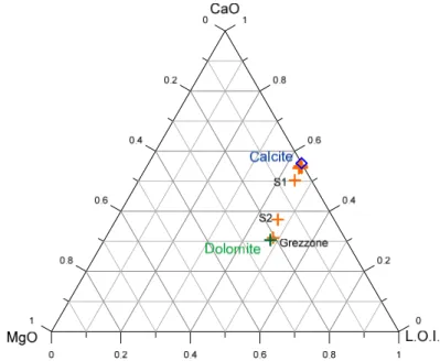
Similar observations arise from the triangular diagrams of:

(i) CaO-MgO-LOI (figure 3.6), where all the rock samples and stream sediment S1 lie close to the point representative of stoichiometric calcite, whereas rock G and stream sediment S2 exhibit a composition similar to that of stoichiometric dolomite;

(ii) CaO-MgO-SiO2 (figure 3.7), in which stream sediment samples are strongly enriched in silica and sample B (black marble) is slightly enriched in silica compared to other lime-rich samples.

Figure 3.4 - CO2 vs CaO diagram showing rocks and stream sediment samples from the study area as well as

the average chemical composition of main rocks (data from TUREKIAN & WEDEPOHL, 1961)

Figure 3.5 - CO2 vs MgO diagram showing rocks and stream sediment samples from the study area as well as

Figure 3.6 – Ternary diagrams LOI, CaO and MgO for the rocks

and stream sediment samples from the study area.

Figure 3.7 – Ternary diagrams SiO2, CaO and MgO for the rocks

and stream sediment samples from the study area.

Finally, results of XRD analysis (Figures 3.8, 3.9 and 3.10) confirm that: (i) calcite is the only mineral recognized in samples A, C, D, I, E, H;

(ii) in addition to calcite, quartz is also present in sample B; (iii) dolomite is the only solid phase detected in sample G.

Figure 3.8 - XRD spectrum of sample A

Figure 3.9- XRD spectrum of sample B

C ount s/s Do lo mi te Do lo mi te Do lo mi te Do lo mi te Do lo mi te Do lo mi te Do lo mi te Do lo mi te Do lo mi te Do lo mi te Do lo mi te Do lo mi te Do lo mi te Do lo mi te Do lo mi te Do lo m it e Do lo mi te Do lo m it e Do lo mi te Do lo mi te Do lo mi te Do lo mi te Do lo mi te Do lo mi te Do lo mi te Do lo mi te Do lo mi te Do lo m it e Do lo mi te Do lo mi te Do lo mi te Do lo m it e Do lo mi te Figure 3.10 - XRD of sample G

3.2.2 – Atmospheric particulate matter and rainwater

Chemistry of atmospheric particulate matter (PM10) was investigated by SEM-EDS analysis (Scanning Electron Microscope - Energy Dispersive X-Ray Spectrometer) at the Microscopy and Microanalysis Interdisciplinary Center (MEMA) of the University of Florence. Data on shape and morphology of atmospheric particles collected on filters were also obtained. In detail, the used electron microscope (ZEISS EVO MA15) is equipped with an OXFORD INCA spectroscopy detector 250 and the software INCA Feature.

The scanning electron microscope (SEM) works with an electron beam generated by an electron gun located on the top of a column containing focusing lenses. The beam scan the filter following parallel lines and causing two main phenomena: 1) the emission of secondary electrons with energies of a few tens of eV from the top layer of the sample, 2) the re-emission or reflection of high-energy electrons or backscattered electrons belonging to the primary beam. In detail, the secondary electrons are used to construct enlarged images while the backscattered electrons are used to identify the presence of different chemical elements as their intensity is a direct function of the average atomic number of the investigated substance.

The distribution of the equivalent diameter (ECD, in μm) of analyzed particles is shown in the following quantile-quantile plots (or qq plots; figures 3.11, 3.12, 3.13).

CARCHIO -4 -3 -2 -1 0 1 2 3 4 Theoretical Quantile 0.01 0.05 0.25 0.50 0.75 0.90 0.99 0 2 4 6 8 10 12 Ob s e rv e d V a lu e

  CORCHIA -4 -3 -2 -1 0 1 2 3 4 Theoretical Quantile 0.01 0.05 0.25 0.50 0.75 0.90 0.99 0 1 2 3 4 5 6 7 8 9 10 Ob s e rv e d V a lu e

Figure 3.12 – Q-q plot of equivalent diameter values for the PM10 sample from Corchia station.

MATANNA -4 -3 -2 -1 0 1 2 3 4 Theoretical Quantile 0.01 0.05 0.25 0.50 0.75 0.90 0.99 0 1 2 3 4 5 6 7 8 Ob s e rv e d V a lu e

Figure 3.13 – Q-q plot of equivalent diameter values for the PM10 sample from Matanna station. Since data sets obtained for each filter do not have a unimodal distribution, but consist of at least three populations, it was decided to split the data set for each filter in three populations according to the following logarithmic scale:

SEM-EDS analysis provides the contents of major constituents (C, O, Na, K, Mg, Ca, Al, Fe, Si, Ti, S, and Cl) and some minor/trace components, including Ni, Mo and Br. Values of carbon and oxygen were eliminated, since these two elements are major constituents of nitrocellulose filters on which particles were sampled. Then, analytical results were re-computed to a total of 100 atomic percentages.

Average contents of Na, K, Mg, Ca, Al, Si, and S in atomic units and the average Si/Al ratio for all the analyses and for each of the three size intervals mentioned above are now presented and discussed.

In the Carchio sample, PM1 (table 3.2), sodium, magnesium, aluminum and silica vary considerably depending on the considered size interval, with a general increase in concentrations with decreasing particle size. In contrast, sulfur, potassium and calcium contents remain approximately constant in the different granulometric classes. Chlorine was not detected in this site.

Table 3.2 - Carchio (PM1)

Na (au) Mg (au) Al (au) Si (au) S (au) K (au) Ca (au) Si/Al

all analyses 1.05 1.21 0.66 1.15 1.41 0.37 0.84 1.75 10-4.64 0.38 0.13 0.34 0.68 1.45 0.36 0.71 2.02 4.64-2.15 0.82 0.52 0.69 1.17 1.34 0.34 0.88 1.71 2.15-1 1.18 1.43 0.77 1.31 1.44 0.40 0.85 1.71

In the Corchia sample, PM2 (table 3.3), sodium, chlorine and potassium contents increase with decreasing particle size. Magnesium and silica concentrations are nearly equal in the two large-size classes, while doubling their values in finest particles. Aluminum, sulfur and calcium contents remain approximately constant in all granulometric classes.

Table 3.3 - Monte Corchia (PM2)

Na (au) Mg (au) Al (au) Si (au) S (au) Cl (au) K (au) Ca (au) Si/Al

all analyses 0.54 0.47 0.66 1.18 1.22 0.29 0.40 1.10 1.77 10-4.64 0.23 0.28 0.60 0.89 1.23 0.11 0.25 1.11 1.48 4.64-2.15 0.43 0.27 0.70 0.86 1.25 0.19 0.37 1.08 1.22 2.15-1 0.58 0.59 0.66 1.37 1.20 0.36 0.44 1.11 2.09

In the Matanna sample, PM3 (table 3.4), sodium, potassium, calcium and chlorine concentrations increase with decreasing size, magnesium and sulfur contents remain approximately constant in all granulometric intervals, aluminum content tends to increase with decreasing size, while silica concentration appears to vary in random way.

Table 3.4 - Monte Matanna (PM3)

Na (au) Mg (au) Al (au) Si (au) S (au) Cl (au) K (au) Ca (au) Si/Al

all analyses 1.83 0.56 0.77 1.53 1.34 0.41 0.27 0.44 1.99 10-4.64 1.42 0.51 0.45 1.95 1.45 0.18 0.36 4.37 4.64-2.15 1.77 0.59 0.53 1.31 1.30 0.19 0.19 0.40 2.45 2.15-1 1.90 0.55 0.84 1.59 1.36 0.73 0.34 0.51 1.89

To analyze further the results of SEM-EDS analyses, some binary and ternary plots were constructed, reporting the composition of relevant mineral phases, in addition to analytical data, which are represented with different symbols, as a function of particle size.

In the Ca vs. S plot for the Carchio site (figure 3.14a) data are generally located between the line of ratio Ca/S = 1, which is characteristic of gypsum and/or anhydrite, and the X-axis, which is characteristic of Ca-free sulphate minerals, such as ammonium sulphate, one of the most likely candidates based on the general knowledge of atmospheric particulate matter (e.g., BERNER & BERNER, 1996). Only two analyses show a

Ca/S ratio > 1, suggesting the presence of calcium sulphate and another Ca-bearing mineral, such as calcite. There is no trend indicating a possible relation between Ca/S ratio and particle size, in agreement with previous observations based on average Ca and S contents in different granulometric classes.

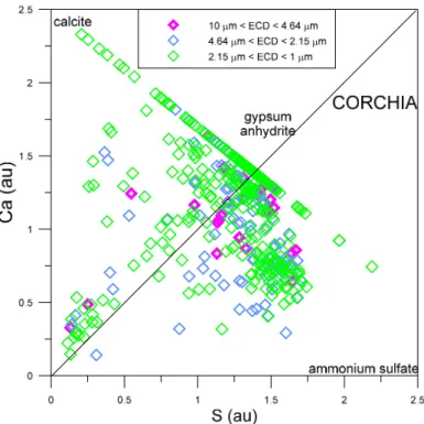
The Ca vs. S diagram for the Corchia site (figure 3.14b) highlights variations of the Ca/S ratio much greater than in the previous case. There are, in fact: (i) particles with Ca/S ratio > 1, attributable to coexistence of calcite and Ca-sulphates, (ii) particles with ratio Ca/S=1, indicative of gypsum and/or anhydrite, and (iii) particles wit Ca/S ratio <1, due to the presence of ammonium sulphate or other Ca-free sulphate minerals. Most particles are distributed in two groups, one along the line of gypsum/anhydrite and the other one characterized by Ca/S ratio close to 0.5. Also in this case there seems to be no preferential distribution suggesting a possible relationship between Ca/S ratio and particle size, in agreement with previous inferences based on mean Ca and S concentrations in different size intervals.

The Ca vs. S plot for the Matanna site (figure 3.14c) shows that the number of available analyses is much smaller than in the previous two cases and the ratio Ca/S ratio is close to 0.25-0.30 for all the analyses, indicating the possible presence of both gypsum and/or anhydrite and ammonium sulphate and/or other Ca-free sulphate minerals.

Figure 3.14a – Ca vs S diagram for the PM10 sample from the Carchio site.

Figure 3.14c – Ca vs S diagram for the PM10 sample from the Matanna site.

The different chemical characteristics of atmospheric particles seem to reflect, at least partly, the diverse lithologies cropping out in the areas where the sampling stations were located. In fact, the presence of calcite in the PM10 from the Corchia site (sample PM2) agrees with the abundance of carbonate outcrops (Marmi and Grezzoni), largely prevailing on Al-silicate rocks of the basement. In contrast, the virtual absence of calcite in the particulate matter from the Carchio and Matanna sites (samples PM1 and PM3, respectively) is in line with the scarcity of carbonate outcrops in these two areas, which are characterized primarily by Al-silicate rocks of the basement, mainly phyllites and porphiroids (Carchio), and metasandstones of the Pseudomacigno formation (Matanna).

Further indications are provided by the ternary plots of K-Al-Si, in which atmospheric dust composition is consistent with that of K-bearing Al-silicates (K-feldspar, muscovite, illite and K-endmembers of clay minerals) although a number of analyses, mainly from the Carchio area (Figure 3.15a) and the Corchia site (figure 3.15b) and subordinately from the Matanna station (figure 3.15c), show an excess of potassium. These particulate matters with anomalously high K concentrations belong to the large granulometric interval (10 μm < ECD < 4.64 μm) in the Carchio site and to the medium and small size ranges (4.64 μm < ECD < 3.15 μm e 3.15 μm < ECD < 1 μm) in the Corchia area. This excess of potassium may be due to anthropogenic pollution (for example use of potassium fertilizers in agriculture) and natural effects (e.g., biogenic

Figure 3.15a – Si-K-Al ternary diagram for the PM10 from the Carchio site.

Figure 3.15c – Si-K-Al ternary diagram for the PM10 from the Matanna site.

The spread of points is similar in the ternary plots of Na-Al-Si, in which several atmospheric particulate compositions compare with those of Na-bearing Al-silicates (albite, paragonite and Na-endmembers of clay minerals) although a considerable number of analyses, chiefly from the Matanna station (figure 3.16c) and subordinately from the Carchio and Corchia area (figure 3.16a and 3.16b, respectively) show an excess of potassium. Excluding the marine origin, due to the virtual absence of chlorine, these enrichments in sodium are attributable to anthropogenic effects.

Figure 3.16a – Si-Na-Al ternary diagram for the PM10 from the Carchio site.

Figure 3.16c – Si-Na-Al ternary diagram for the PM10 from the Matanna site.

As mentioned above, concurrent with the sampling of atmospheric particulate matter, three rainwater samples were also collected, one from each station. Again, pH and electrical conductivity, EC (table 3.5), were measured on site, whereas the concentrations of major dissolved constituents (reported in tables 3.5 and 3.6, in weight units and equivalent units, respectively) and the 18_O/16_{O and} 2_H/1_{H isotopic ratios (table} 3.5) were determined in the laboratories (see section 3.1.2 for further details).

Table 3.5 – pH, EC, chemical data (expressed in ppm) and isotopic data of rainwater samples.

Code Site pH μS/cm EC Cl NO3 SO4 HCO3 Ca Mg Na K δ18_{O δ}2_H

μs/cm (ppm) (ppm) (ppm) (ppm) (ppm) (ppm) (ppm) (ppm) VSMOW) (‰ vs- VSMOW) (‰ vs-PM1 Carchio 4.79 48.9 2.87 3.73 2.01 3.66 1.05 0.37 2.87 0.22 -7.97 -52.08 PM2 Corchia 4.75 35.8 4.24 5.17 2.63 3.66 0.35 0.25 1.95 0.12 -7.89 -54.54 PM3 Matanna 4.40 50.2 5.53 7.16 2.65 3.66 1.00 0.76 3.77 0.41 -8.26 -57.00

Table 3.6 -Chemical composition (expressed in meq/l) of rainwater samples.

Codice Site Cl NO3 SO4 HCO3 Ca Mg Na K

(meq/l) (meq/l) (meq/l) (meq/l) (meq/l) (meq/l) (meq/l) (meq/l) PM1 Carchio 0.08 0.06 0.04 0.06 0.05 0.03 0.12 0.006 PM2 Corchia 0.12 0.08 0.05 0.06 0.02 0.02 0.08 0.003 PM3 Matanna 0.16 0.12 0.06 0.06 0.05 0.06 0.16 0.010

predominant anion and cation are chloride and sodium, respectively, for all three samples. Therefore, these rainwaters belong to the sodium chloride facies (see the following chapter on the classification of waters), as commonly observed in coastal areas. However, nitrate concentrations are also considerable, being slightly lower than those of chloride ion. High nitrate concentrations may be due to different processes, such as oxidation of N compounds (NH3, N2O, NO, etc.) and fossil fuel combustion (BERNER & BERNER, 1996).

By comparing the chemical composition of rainwater with that of particulate matter, it is evident that there are considerable differences, attributable to either lack of interaction between rainwater and particulate matter or fractionation effects. For instance, the Ca/S ratio in the rainwater sample of Matanna does not match the Ca/S ratios found in airborne particles. Occurrence of NaCl dissolution (from sea spray) is possible, considering its absence in atmospheric particulate matter and its relative abundance in rainwater.

Summing up, it can be stated that particulate matter seems to reflect, at least partly, the lithologies cropping out in the area. It is also possible to recognize the effects of anthropogenic pollution at altitudes of roughly 700-850 m a.s.l., in relatively remote areas, and this is not a reassuring perspective. It is difficult to explain compositional differences between rainwater and particulate matter due to the limited number of collected samples.

3.2.3 – Groundwater geochemistry and isotopic ratios

Geochemistry

Groundwater geochemistry is an interdisciplinary science concerned with the chemistry of water in the subsurface environment. The chemical composition of groundwater is the combined result of the composition of water that enters the groundwater reservoir and reaction with minerals present in the rock that may modify the water composition (APPELO & POSTMA, 1996). Groundwater geochemistry has a

potential use for tracing the origins and the history of water. The water quality provides information about the environment through which the water has circulated concerning residence times, flowpath and aquifer characteristics.

After groundwater sampling and analysis the springs have been classified to individuate and distinguish the different families present in the area due to water-rock interaction and other processes.

Based on the ternary plots involving major anions and cations and LANGELIER-LUDWIG

diagrams (1942) it is possible to distinguish the main groups of water with distinctive chemical composition.

Figure 3.17 - Triangular diagrams (a) HCO3-Cl-SO4 e (b) Ca-Mg-(Na+K) for the Alpi Apuane springs.

The ternary diagram of major anions (figure 3.17a) shows that most waters are dominated by HCO3 whereas SO4- and Cl-rich waters are less abundant. The ternary diagram of major cations (figure 3.17b) highlights the prevalence of Ca- and Na-rich waters as well as the presence of three samples characterized by Ca/Mg ratio close to 1.

These observations are confirmed by the square diagram of LANGELIER-LUDWIG

(figure 3.18) whereas the correlation plot of HCO3 vs. SO4+Cl (figure 3.19) provides further details on water salinity.

Figure 3.18 - LANGELIER-LUDWIG diagrams about Alpi Apuane springs.

Figure 3.19 - Correlation diagram of HCO3 vs. SO4+Cl for the Alpi Apuane springs: a) full scale and b)

exploded view diagram. This plot is equivalent to a cross section of the Langelier-Ludwig compositional pyramid with horizontal trace in the square plot of Fig. 3.17, representing the base of the pyramid.

Based on previous diagrams (figures. 3.17, 3.18 and 3.19), it is possible to individuate the following chemical facies:

- Ca-HCO3 waters. These waters are the most numerous in the study area and present a Total Ionic Salinity (SIT) ranging from 4 to 12 meq/l. Samples belonging to this geochemical facies are GB/05, GM/05, LP/05, MS/05, ML1/05, ML2/05, PS1/05, PS2/05, RF/05, CR/09, GB/09, LP/09, MR/09, MS/09, ML1/09, ML2/09, ML3/09, PS1/09, PS2/09, RF/09, SA/09, PN/10, LP/10, CR/10, PS2/10, MS/10, RF/10, ML1/10. - Na-Cl waters. These waters have the lowest SIT values, ranging from 0.92 to 2.66

meq/l. Rainwaters and samples AZ/05, BD/05, SG/05, AZ/09, BD/09, FP/09, MT/09, PC/09, SG/09 and TR/09 belong to this chemical facies.

- Ca-SO4 waters. These water have the highest SIT, varying from 19.9 to 23.4 meq/l. Samples ascribable to this geochemical facies come from the Porta’s Springs (PR1/05, PR2/05, PR2/09, PR3/05, PR09, PR/10).

- Intermediate waters (Ca-HCO3-Cl; Ca-HCO3-SO4; Ca-Mg-HCO3). These waters have both chemical composition and SIT (1.54 to 5.84 meq/l) intermediate with respect to those of previous chemical types. Therefore, they could be produced through either mixing between the previous Ca-HCO3, Na-Cl and Ca-SO4 waters or interaction with different lithotypes.

The geological map of figure 3.20 shows that:

(i) Ca-HCO3 springs are located where carbonate rocks (Marmi, Grezzoni and Calcare Cavernoso) crop out;

(ii) Na-Cl springs are positioned at the contact between thin alluvium deposits and underlying impermeable rocks, usually the lower phyllites formation;

(iii) Ca-SO4 springs are situated near the Porta resort only, where both Calcare Cavernoso and Calcare and Marne a Rhaetavicula contorta crop up.

Figure 3.20 – Simplified geological map of the study area showing the location of sampled spring and their

chemical facies.

All the sampled springs have very low boron and fluorine concentrations, ranging from 0.01 to 0.05 ppm and 0.016 to 0.34 ppm, respectively. The Porta’s springs have the highest B and F contents.

Measurable arsenic concentration ranges from 0.1 to 3.9 ppb, but As concentration is lower than detection limit (0.1 ppb) in 13 samples.

Zinc concentration is usually below 6 ppb, except for samples MT and GM, whose Zn contents are 29 and 10 ppb, respectively.

Concentrations of chromium, copper, manganese, nickel and lead are very low and near the detection limit, which is 1 ppb for all these elements.

Iron concentration ranges from 1 to 8 ppb, except sample ML2/09 that has 126 ppm Fe. However, the same springs sampled a second time presents iron concentration of 2 ppm. So, the higher value measured the first time could be related to a technical problem. Accepting that dissolved Fe is prevailingly present in the trivalent redox state, its content appears to be limited by saturation with a sparingly soluble oxy-hydroxide of Fe(III), in agreement with low measured concentrations. As a matter of fact, in the Eh-pH plot for the Fe-O-H system (figure 3.21), sampled springs are situated in the stability

field of hematite, representing a proxy for amorphous Fe(OH)3 or poorly crystalline ferrihydrite, in line with previous considerations.

Figure 3.21 - Eh-ph diagram for the Fe-O-H system (from Takeno, 2005) reporting the analytical

values for all the sampled springs (circles).

Finally, silica concentration varies from 0.85 ppm (in sample LP) to 11.3 ppm (in sample MT). In the graph of SiO2 vs. temperature (Figure 3.22) a general tendency of increasing silica content with temperature is recognizable. In addition, several Ca-HCO3 waters are undersaturated with quartz, in line with short interaction with silica-poor carbonate rocks only, whereas other samples are oversaturated with quartz and undersaturated with chalcedony, indicating either longer interaction times with carbonate rocks or acquisition of silica through dissolution Al-silicate minerals contained in rocks different from carbonate lithotypes.

Figure 3.22 – Temperature-silica diagram showing analytical values for all the sampled springs as well

as quartz and chalcedony solubility lines (from FOURNIER, 1973).

Isotope geochemistry

Isotopes are atoms whose nuclei contain the same number of protons but a different number of neutrons. The term “isotope” is derived from Greek, meaning equal place, and indicates that isotopes occupy the same position in the periodic table. Isotopes can be divided into two fundamental kinds: stable and instable.

In this study only stable isotopes are used, namely the 2_H/1_{H and} 18_O/16_{O isotopic} ratios of H2O and the 13C/12C isotopic ratio of Total Dissolved Inorganic Carbon (TDIC).

The stable isotope ratios are expressed in δ‰, that is the difference per thousand between the sample isotopic ratio compared to reference standard:

1000

1

R

R

‰

_⋅

⎟⎟

⎠

⎞

⎜⎜

⎝

⎛

−

=

δ

where Rstandard e Rsample are the isotopic ratio of 18O/16O o 2H/1H o 13C/12C related to standard and to sample respectively.

The standard used for isotopic ratios 18_O/16_{O e} 2_H/1_{H is V-SMOW (Vienna Standard} Mean Ocean Water), which represents the average value of the isotopic composition of ocean waters, which are the start and end of the hydrological cycle (by definition of δ‰ V-SMOW is equal to zero). The reference standard for the isotopic ratio 13_C/12_{C is instead} the Vienna Pee Dee Belemnite (VPDB).

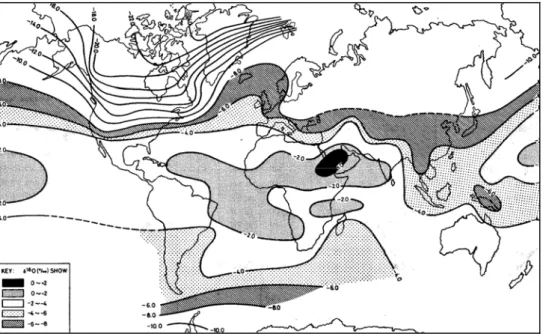
As a result of various evaporation and condensation processes, which occur during the hydrological cycle, the waters are affected by isotopic fractionation and thus by changes in composition primarily evidenced by isotopic ratios 18_O/16_{O e} 2_H/1_{H. In} particular during the evaporation process that water vapour that is released is significantly poorer in heavy isotopes (δ‰ lower) than the water from which it originated. Whereas during the condensation the liquid phase is richer in heavy isotopes (δ‰ higher) than the mass of vapour from which it originates. The result is that the rainwaters within mainland, originated from vapour depleted in heavy isotopes due to the succession of condensations, are isotopically lighter than coastal rainwater. Another factor that affects, significantly, the values of δ2_{H‰ e δ}18_{O‰ in the rainwater is the} temperature, and this is the cause for which the isotopic ratio of precipitation varies with latitude, altitude and with seasons. In fact, the waters tend to be isotopically lighter with increasing latitude and altitude and, moreover, the average summer rainwater have an isotopic ratio heavier than winter (figures 3.23 and 3.24).

Figure 3.23 – Distribution at different latitude of 18_O/16_{O medium value in rainwater}

Figure 3.24 – Seasonal variations in isotopic composition of rainwater

(from YURTSEVER &GAT, 1981).

The amount of rainwater affects the isotopic ratio, in particular the most abundant rains are relatively poor in heavy isotopes.

A further characteristic regarding 2_H/1_{H e} 18_O/16_{O of rainwater is to be correlate by} a linear relationship with general expression δ2_H‰=A*δ18_{O‰+d, where "d" represents} the excess of deuterium. The slope of the line (A) generally is equal to 8, while the deuterium excess may vary from region to region. Particularly in the Mediterranean basin, the term "d" is generally between +12 and +15. Water characterized by a content in stable isotopes that deviate from the straight line may indicate phenomena of evaporation or water rock interactions at high temperature (above 200°C) or addition of water with particular isotopic ratio (eg. water magmatic ).

Differences in chemical and physical properties arising from variation in atomic mass of an element are called “isotopic effects” (HOEFS, 2004). For a more detailed

introduction to “isotope effects” and related isotope fractionation mechanisms see specific literature (CRAIG, 1961a-b; DANSGAARD, 1964; GAT & CARMI, 1970; GAT, 1980; 1981; FRITZ

& FONTES, 1980; GONFIANTINI, 1981; YURTSEVER & GAT, 1981; CLARK & FRITZ, 1997; KENDALL

& MCDONNEL, 1998 for general characterization PANICHI et al., 1974; BORTOLAMI et al.,

1978; FONTES et al., 1978; ANOVSKI et al., 1985; CELATI et al., 1991; D’AMELIO et al.,

1994; GRASSI, 1994; MUSSI et al., 1998; KATZ et al., 1998; RADEMACHER et al., 2002;

BARBIERI et al., 2003 for their applications).

Since 1960, 2_H/1_{H and} 18_O/16_{O isotope ratios have been used in hydrogeological} studies, as knowledge of the isotopic composition of rainwater is an important tool for

hydrological, hydro-meteorological and climatological researches. In particular, applications of isotopic techniques require two fundamental types of data: a map of the distribution of 2_H/1_{H and} 18_O/16_{O isotope ratios in rain waters and the vertical isotopic} gradient typical of the area of interest (LONGINELLI & SELMO, 2003, DOTSIKA et al., 2010).

LONGINELLI & SELMO (2003) have reconstructed the isotopic map of Italy (figure

3.25), based on data from 77 different locations, where composite monthly samples of precipitation were taken over time intervals ranging from one to seven years. These authors have shown that:

(i) no latitudinal isotopic gradient exists from Sicily to the Italian-French border, despite the latitudinal extension of the Tyrrhenian coast of Italy;

(ii) the mean vertical isotopic gradient is -0.2‰/100m, confirming the work of DANSGAARD (1961);

(iii) the equation relating amount-weighted mean oxygen isotope value to mean hydrogen isotope value shows quite a large range of values for both the slope (from 5.7 to 8.9) and the deuterium excess (from +9.2 to +19.1 ‰) for individual stations. This is due to both the peculiar position of Italy in the Mediterranean Sea and the presence of two mountain chains crossing it along two very different directions, roughly NW-SE and E-W.

The “altitude effect” was first described by DANSGAARD (1961) who observed that

the 18_O/16_{O value of rain water shows a decrease close to 0.2‰ units for every hundred} m of elevation gain in temperate regions. Although the huge work done by LONGINELLI &

SELMO (2003) represents a giant step forward in stable isotope geochemistry, its scale is

not sufficient for most local studies. In fact, an exhaustive knowledge of the isotopic composition of local precipitations and how it is related to local environmental conditions is essential for hydrological studies on a local scale. This aspect will be discuss in the next section.

Figure 3.25- Distribution map of δ18_{O values for Italian rainwaters}

(from LONGINELLI & SELMO, 2003).

Values of δ2_{H and δ}18_{O of the Apuan springs together with some rains collected in} the study area are shown in the correlation diagram of figure 3.26. The plot confirms that all the collected waters are of meteoric origin; consequently, it can be concluded that differences in 2_H/1_{H and} 18_O/16_{O isotopic ratios mainly depend on infiltration altitude.}

However, δ2_{H and δ}18_{O values of Apuan springs and rains fit the following linear} regression equation (r=0.789):

δD=7.39 ⋅ δ18_{O + 4.99,}

which is somewhat different from both the worldwide meteoric line for rainfall defined by CRAIG (1961):

δD = 8 ⋅ δ18_{O + 10}

and the “Apuan characteristic line” determined by MUSSI et al. (1998):

Figure 3.26 – Diagram of δ2_{H vs. δ}18_{O values for sampled springs and rainwaters.}

The 13_C/12_{C isotopic ratio of TDIC is a tool to determine the provenance of carbon,} which can be related to different sources, including atmospheric CO2, decomposition of organic matter and dissolution of carbonate rocks (CRAIG, 1953). Ranges of the 13C/12C

isotopic ratio for these different sources of carbon are as follows:

(i) from -7 to -8 ‰ vs. VPDB for the atmospheric source (HOEFS, 2004);

(ii) from 0 to +2 ‰ vs. VPDB for the dissolution of carbonate rocks (DEINES et al., 1974;

CHIODINI et al., 2000);

(iii) from -20 to -25 ‰ vs. VPDB for the biogenic source (DEINES et al., 1974; DEINES,

1980; CERLING et al., 1991; ROBINSON & SCRIMEOUR, 1995; CLARK & FRITZ, 1997; CHIODINI

et al., 2000).

To estimate the contribution of these different components for the Apuan groundwaters a suitable exercise of geochemical modelling was performed (figure 3.27). Initially, addition of biogenic CO2 to average meteoric water with a δ13CTDIC value of -5.5±0.5‰ (FRONDINI, 2008) and TDIC of 7±2 mg HCO3/L was calculated (solid line in figure 3.27), adopting two different δ13_C

TDIC values for thebiogenic CO2 (-20 and -25 ‰). Then starting from two Na-Cl waters, whose δ13_C

TDIC values and TDIC concentrations are closely approximated by addition of biogenic CO2 to the average meteoric water, addition of biogenic CO2 coupled with calcite dissolution was modelled (dotted line in figure 3.27) by means of the EQ3/6 software package (WOLERY & JAREK, 2003). In this way, it was

modelling the δ13_{C value of calcite was assumed equal to the mean value of sampled} rocks (+1‰) (see paragraph 3.1.1).

Geochemical modelling highlights that: (i) δ13_C

TDIC values and TDIC concentrations of Na-Cl and possibly Ca-HCO3-Cl waters are explained by addition of biogenic CO2;

(ii) δ13_C

TDIC values and TDIC concentrations of samples belonging to other chemical facies also implies calcite dissolution driven by addition of biogenic CO2.

Figure 3.27 – Diagram of δ13_C

TDIC value vs. TDIC concentration for the sampled Apuan springs also showing the

theoretical effects expected for addition of biogenic CO2 to average meteoric water and calcite dissolution driven by addition of biogenic CO2 to two selected Na-Cl springs.

Hydrochemistry and stable isotope in karst aquifers

The application of isotopic ratios, like 2_H/1_{H and} 18_O/16_{O of H}

2O and 13C/12C of Total Dissolved Inorganic Carbon (TDIC), as conservative tracers in the investigation of hydrological processes occurring in water catchments has become a common tool in the last decades (FRITZ & FONTES, 1980; MAZOR, 1991; KENDALL & CALDWELL, 1998). Isotope

techniques are of particular value when examining fracture flow hydrology since these systems are difficult to treat using conventional hydrologic models (ROSE et al., 1996).

As specified above, application of isotopic techniques requires two fundamental data: a map of the distribution of 2_H/1_{H and} 18_O/16_{O ratios in rain water and the vertical} isotopic gradient typical of the area of interest (LONGINELLI & SELMO, 2003, DOTSIKA et al.,

2010). Generally these data are obtained through a system of rainfall stations that allows one to collect mean monthly and annually weighted values for a period of at least three years. When isotopic data regarding rain falls are limited or not available, it is possible to use a different approach to the problem, focussing on the isotopic characteristics of spring waters of rapid flow and small circuit, with discharge elevations not very different from infiltration altitudes (CELICO, 1986; MAZOR 1991). In addition, it is advisable to carry

out repeated surveys, to take into account possible seasonal variations reflecting the isotopic changes of the rains recharging these groundwater circuits. This methodology was used by MUSSI et al. (1998) in the Alpi Apuane-Garfagnana area for which the

authors showed the presence of an isotopic gradient lower than those usually found. This is most probably due to the rather particular arrangement of the reliefs and to the preferential direction of atmospheric disturbances (MUSSI et al., 1998).

Based on previous geochemical considerations it is possible distinguish two main types of circulation: (i) circuits hosted in carbonate rocks or carbonate-evaporite formations and (ii) shallow circulations in screeds or semi-permeable rocks.

The circuits of the first type involve rocks of by high permeability, like marble, dolomitic marbles and Grezzoni, and discharge through Ca-HCO3 and Ca-SO4 springs of high flow rate. In detail, Ca-HCO3 waters proceed from shallow circuits mainly hosted in fractured and karstified carbonate rocks whereas Ca-SO4 waters are representative of relatively deep circuits in carbonate-evaporite formations. These waters are close to saturation with respect to dolomite and calcite and their δ13_C

TDIC values are consistent with calcite dissolution governed by biogenic CO2. All these springs are typical of karst aquifers and have both comparatively long flow paths and relatively prolonged water-rock interaction histories.

The circulations of the second type, hosted in screeds with primary permeability or in sparingly permeable rocks, discharge waters of usually low flow rate (<0.5 l/s) and low salinity, either with Na-Cl composition or intermediate characteristics. These immature waters are typical of shallow circulations and can be considered as representative of slightly evolved, rapidly circulating rains. Among the springs sampled in this study, the low-discharge springs AF, AZ, BD, FC, FP, GM, LL, ML3, MT, PC, SG, TR and ZP were selected to calculate the mean isotopic vertical gradient of the study area. For each the mean infiltration altitude is been evaluated based on the litology of cropping rocks and on morphology.

In this way, a mean vertical isotopic gradient of -0.17‰/100 m (figure 3.28) was obtained for oxygen isotopes, considering the average 18_O/16_{O isotopic ratio of the two}

The obtained isotopic gradient is similar to that found by LONGINELLI & SELMO (2003)

for different Italian areas (-0.2 ‰/100 m), confirming the need for a local calibration of the isotope-altitude relation.

In figure 3.27, the altitude - δ18_{O‰ relationship, computed for the study area} considering a congruous number of selected low-discharge springs, is used to evaluate the mean infiltration altitude of high-flowrate springs, based on their δ18_{O values.}

Figure3.28 – Correlation between mean infiltration quote and 18_{O ratio (blue line). The correlation was}

determined using the “low-discharge” springs (green triangle); for “high-flowrate” springs (blue cross) the mean infiltration altitude was evaluate.

3.2.4 – Speciation calculations and saturation state

The term “chemical speciation” refers to the equilibrium distribution of ionic forms and of neutral complexes that compete to define the global chemical composition of the aqueous phase. It is important to know the chemical speciation of dissolved constituents to study the balance between aqueous solution and mineral phases present in the rocks and so to assess the state of saturation of the aqueous solution with respect the solid phases. The chemical speciation is calculated by means of automatic calculation routines, leading to convergence the thermodynamic constants relative to homogeneous equilibrium in aqueous phase, the relative mass balance for the dissolved components and the charge balance (OTTONELLO, 1991, 1997). The computer code used in this thesis

is the program EQ3, which is part of the software package EQ3 / 6, version 8.0 (WOLERY

& JAREK, 2003), initially proposed by WOLERY (1979).

The input data are the analytical concentrations of the chemical species present in the solution and other parameters such as pH, temperature and Eh or, alternatively, another variable/condition which describes the redox state of aqueous solution. For multi-valent elements (eg Fe), it is possible to:

(i) enter as input the total concentration (eg, total Fe), taking the form of redox equilibrium, although it is rarely a constraint reasonable for natural waters (eg, LINDBERG

& RUNNELS, 1984);

(ii) specify the concentration of the different redox forms (eg, Fe bivalent and Fe trivalent), taking the form of redox imbalance.

To understand the essence of speciation calculations it is possible to consider the case of calcium, whose total molal concentration is the sum of the molality concentrations of all ionic species or neutral calcium-containing, and so:

mtotCa = mCa2+ + mCaOH+ + mCaCO3 + mCaHCO3- + mCaHPO4 +…+

since it is possible write an equation very similar to the one above for each of the dissolved components n, n equations exist. These equations indicate precisely the total molality of the solute in relation to those of its various ions and aqueous complexes.

The mass balance equations are associated with the charge balance, which expresses the overall neutrality of the solution:

The activities of various ionic species are controlled by a large numbers of homogeneous balances, for example taking into account the complex CaOH+ _{we have:}

CaOH+ _{ÅÆ Ca}2+ _{+ OH}-

expressing the thermodynamic equilibrium constant of the previous dissociation reaction in terms of molality concentrations, for example mCa2+, and activity coefficients, for example γCa2+, we obtain:

log K = log mCa2+ + log mOH- - log mCaOH+ + logγCa2+ + log γOH- - log γCaOH+ The individual activity coefficients of ionic species can be calculated Debye-Huckel approach or the Davies equation:

Or B-dot equation:

.

In these equations, Aγ and Bγ are functions of the dielectric constant and density of the solvent and of the temperature, z is the charge of aqueous species, the ion-size parameter å, B-dot is an empirical parameter characteristic of each electrolyte and I is the ionic strength, which is defined by the following equation:

2 i i i

z

m

2

1

I

=

∑

⋅

As regards the neutral species, the activity coefficient takes on unit value in the equation of Davies, while the B-dot equation reduces to:

However, following GARRELS & THOMPSON (1962), HELGESON (1968), and HELGESON et

aqueous in solutions of pure NaCl of the same ionic strength. Alternatively, it is possible calculate the activity coefficients of aqueous species using the equations of Pitzer (WOLERY

& JAREK, 2003 and related references).

The knowledge of the thermodynamic constants and of the activity coefficients, at the conditions of pressure and temperature requirements, allows to determine the speciation of the aqueous solution, solving the system of equations of interest, by means of automatic procedures for convergence. In the case of EQ3/6 is used the Newton-Raphson method, although there are others (WOLERY & JAREK, 2003 and related

references).

Once reconstructed speciation, the EQ3 code computes the conditions of saturation of the aqueous solution with respect to mineral phases of interest. Taking into consideration the case of calcite, it is possible to write:

calcite + H+ _{= Ca}2+ _{+ HCO} 3-

The saturation index (SIcalcite) with respect to this phase is defined as:

calcite H calcite HCO Ca calcite calcite

calcite

log

log

K

K

Q

log

SI

−

⋅

⋅

=

⎟⎟

⎠

⎞

⎜⎜

⎝

⎛

=

a

a

a

a

Qcalcite is the activities product of the ions;

Kcalcite is the thermodynamic equilibrium constant.

So the water saturation state respect to the i-species mineral of interest is described by the saturation index, which is determined by the following formula:

(

)

i

log

Q

K

SI

=

For SI = 0 there is equilibrium between the mineral and the solution; SI <0 reflects undersaturation and SI <0 supersaturation. Different types of information can be obtained from saturation data. Normally equilibrium is not found and then the saturation state merely indicates in which direction the processes may go: for undersaturation dissolution is expected and supersaturation suggests precipitation. Occurrence of precipitation may be hindered by non-thermodynamic constraints, e.g., slow kinetics of nucleation and/or growth of the solid phase of interest. However, dissolution of the

In the next paragraphs the water saturation index with respect to calcite, dolomite, anorthite, albite, K-feldspar, diopside, gypsum and anhydrite are taken into account. To consider the possible errors on analytical data, thermodynamic constants and speciation calculations, an uncertainty of 0.2 units on the saturation index has been adopted. So, SI <-0.2 reflects undersaturation, SI >+0.2 describes supersaturation, whereas SI between -0.2 and +0.2 outlines the condition of equilibrium (saturation).

Correlation diagram PCO2-pH

The pH values reflect the balance between the input of acidic aqueous solutions and their consumption, generally water-rock interaction. The main acids present in natural waters are CO2, which generate carbonic acid (H2CO3), and organic acids (eg humic acids and fulvic acids). Both the CO2 and organic acids are originated mainly in soils through decomposition processes of organic matter mediated by bacteria. Locally, the CO2 can also have a deep origin, while the contribution of atmospheric CO2 is usually negligible. Acids dissolved in natural waters are gradually neutralized by interaction with minerals in the rocks. This neutralization process results in a first step in which occur the conversion of H2CO3 in to HCO3- and then the conversion HCO3- in to CO32-. So the pH is partially influenced by the degree of advancement of the water-rock interactions. Especially low pH are due to the inability of the rocks to neutralize of acid or to a little interaction with lithotypes hosting the aquifer.

To build the PCO2-pH diagram is required concentration of total dissolved inorganic carbon (TDIC) and the partial pressure of CO2, which were obtained by calculation of speciation-saturation, mainly based on data of pH and alkalinity.

The figure 3.29 shows the pH-PCO2 diagram relating to springs collected in the area of interest with the addition of iso-lines of TDIC, calculated using the following simplified relationship:

⎟

⎟

⎠

⎞

⎜

⎜

⎝

⎛

⋅

+

+

⋅

=

10

K

K

10

K

1

K

m

P

This equation is easily obtainable by the equilibrium of carbonate, which is based on: (i) the equilibrium reaction between carbon dioxide and gaseous CO2:

H2CO3 = CO2(g) + H2O

whose equilibrium constant, KH, is equal to 101.47 atm/(moli/kg) a 25°C, 1 atm; (ii) the dissolution reaction of carbonic acid:

H2CO3 = HCO3- + H+

whose thermodynamic equilibrium constant,

3 2CO H

K

(iii) the dissolution reaction of bicarbonate ion: HCO3- = CO32- + H+

whose thermodynamic equilibrium constant, − 3 HCO

K

(iv) the mass balance on the TDIC:

− −

+

+

=

m

m

m

m

As it is possible to see from the diagram, the logarithm of PCO2 is strongly related to

pH differently for each chemical facies, because the two variables are related by the following equation:

⎟⎟

⎟

⎠

⎞

⎜⎜

⎜

⎝

⎛

γ

⋅

⋅

⋅

+

γ

⋅

⋅

=

10

K

K

2

10

K

alk

K

P

that can be applied below or above pH 8.3, until hydroxyl ion and other weak bases becomes important (neglected for simplicity). However, for the water with a pH below 8.3 (for which alkC = −

3 HCO

m

3 2 3 3 2 CO H HCO HCO pH H CO

K

m

10

K

P

⋅

γ

⋅

⋅

=

.

Specifically, the PCO2-pH diagram shows that, regardless of the chemical facies, the pH of groundwater ranging from 6 to 8.4 and the PCO2 from 0.0005 to 0.038 bar, with a decrease in PCO2 with an increasing the pH. Rainwater sample rather have pH values between 4.79 and 4.4 and PCO2 ranging between 0.054 0.17 bar. The diagram shows two main trends of evolution, both PCO2 decreased with increasing pH: the first, characterized by TDIC values of about 100-300 mg HCO3/L, including the waters of relatively evolved composition of Ca-SO4, Ca-HCO3-SO4, Ca-HCO3, Ca-Mg-HCO3 and the second one, with TDIC content between 10 and less than 100 mg HCO3/L, characterized by immature waters (ie waters that have not interacted sufficiently with the lithotypes present in this

Figure 3.29 – PH vs PCO2 correlation diagram. In the diagram are also reported some iso-TDIC-line and the

Correlation diagram pH – calcite saturation index

In the diagram of correlation between pH and saturation index with respect to calcite (figure 3.30), the groundwater collected are distributed in the two groups already recognized in the previous diagram. In detail, the high-TDIC waters, belonging to the facies calcium bicarbonate and calcium sulphate, are generally saturated or supersaturated in calcite, while the low-TDIC samples belonging to the facies Na-Cl and Ca-HCO3-Cl appear to be strongly undersaturated in calcite, Ca-HCO3 water Ca-SO4, Ca-Mg-HCO3 and some samples of Ca-HCO3 facies occupy an intermediate position, with less marked undersaturation.

Considering the speed with which natural waters reaches the saturation state of calcite, due to its high dissolution rate, it is probable that these waters, undersaturated and with low TDIC, are related to circuits that develop within lithotypes where calcite is virtually absent or are related to a extremely fast circuits.

To explain the pH dependence of the saturation with respect to calcite for waters in question (referring to the composition of Ca-HCO3 waters that make up the largest group), it is possible to write the reaction of dissolution of calcite in the two following forms: − + +

₌

₊

+

H

Ca

HCO

CaCO

2

H

Ca

H

CO

CaCO

+

=

+

Consequently, the dependence SIcalcite-pH can be expressed as follows:

( HCO

Ca

calcite

pH

log

log

logK

I

S

+

−

+

=

a

a

calcite

2

pH

log

log

logK

I

S

+

−

+

⋅

=

a

a

The theoretical slope of the relationship between SIcalcite and pH is 1 for reaction (1) and 2 for (2). The observed value of 0.85, for the waters belonging to the Ca-HCO3 facies is close to the theoretical slope of the first reaction, which therefore seems to be more suitable to describe the process of dissolution/precipitation of calcite.

Figure 3.30 – pH vs SIcalcite correlation diagram.

The diagram in figure 3.31, where are reported only Ca-HCO3 water present in the study area, contrasts the logarithm of PCO2 with the saturation index of waters with respect to calcite. For an isothermal process there is a linear relationship between log PCO2 and SIcalcite with a slope of -1. To explain this dependence, it is necessary to refer to the reaction of dissolution of calcite, written in the following form:

CaCO3 + CO2(g) + H2O = Ca2+ + 2 HCO3-. So the SIcalcite is defined as follows

K

log

log

2

m

log

2

log

m

log

P

log

SI

=

−

+

+

γ

+

⋅

+

⋅

γ

−

Assuming that the ion activity coefficients of HCO3- and Ca2+ are close to unit, this simplified equation is obtained:

)

K

log

m

log

2

m

(log

P

log

SI

=

−

+

+

⋅

−

It explains the linear relationship with a slope of -1 between SIcalcite and log PCO2, assuming that the molalities of HCO3- ion, Ca2+ ion and temperature do not undergo

marked variations. In addition, at saturation with calcite (SIcalcite = 0), the following relation is valid:

K

log

m

log

2

m

log

P

log

=

+

⋅

−

.

Based on a purely statistical approach, the two alignments observed in figure 3.31 for the springs circulating in the carbonate rocks of both the Apuane Unit, mainly Marmi and Grezzoni (blue crosses), and those of the Tuscan Nappe (purple crosses), mainly limestones, can be described by means of simple regression lines (black lines), although the distribution of points results from the superposition of the two following processes:

(i) Dissolution of calcite, which takes place when SIcalcite <0, as shown for two undersaturated samples (gray dotted lines). The process can be described referring to the two limiting models of open-system and closed-system with respect to CO2. In the first case, CO2 is supplied continuously to the aqueous solution, which is considered to be connected with a virtually infinite reservoir of this gas, maintaining a constant PCO2 during the process. In the second case, CO2 supply takes place in a single event, before beginning of calcite dissolution, which causes a gradual decrease in PCO2. It is evident that the compositional evolution is significantly different, in terms of solute concentrations and pH, whether calcite dissolution takes place under open-system or closed-system conditions.

(ii) Degassing, which involves a progressive CO2 loss and the consequent increase in SIcalcite. It is reasonable to assume that: (i) gas loss is favoured by both presence of karst cavities connected with the atmosphere and water turbulence within these cavities, whereas (ii) water circulation in small fractures does not trigger gas loss. Consequently, extent of degassing depends on the type of underground circulation.