Chapter 5 Analysis of beam-to-column connections

(1)

Chapter 5 Analysis of beam-to-column connections

5.1 Abstract

Several tests have been simulated to beam-to-column connections. At first a beam-to-column connection has been extrapolated from the X-Z frame of Building 1 [see Chapter 7], and modeled using different possibilities provided by OpenSees. Monotonic and cyclic plane analysis have been performed in X-Z plane. Then other connections have been modeled and analyzed, with the special aim of investigating the influence of material and geometrical parameters on the behavior of the connection itself.

In Chapter 6 deterioration models have been used and the analysis have been compared to real tests performed by the Department of Steel Construction of RWTH Aachen University within a research project for modern plastic design of steel structures, named PLASTOTOUGH [19].

5.2 Material and geometry of the tests

The strain-stress diagram of steel S235, used in the following OpenSees models, is shown below.

Fig. 5.1 – Material S235 – stress-strain curve

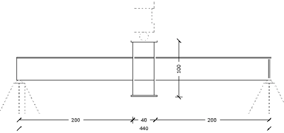
The geometry and the common features of all the models are shown in the next images

(2)

Fig. 5.3: Beam to column connection - geometric characteristics

Fig. 5.4: Beam to column connection – 3D view [SAP2000]

5.3 OpenSees materials used

To ensure a non linear behavior of the column only non-linear behavior material have been considered. Specifically:

 Uniaxial Material Hardening

 Uniaxial Material Steel01 [ref. par. 3.5]  Uniaxial Material Steel02 [ref. par. 3.5]

 Modified Ibarra-Medina-Krawinkler deterioration model with bilinear hysteretic response [ref. par. 3.9]

5.4 OpenSees sections used

The sections used to model the non linear behavior of the cconnection have been:  Fiber section [ref. par. 3.6]

 Zero-length section [ref. par. 3.6]

5.5 OpenSees elements used

The element used to model the non linear behavior of the column have been:  Elastic Element [ref. par. 3.7]

 Nonlinear Beam-Column Elements [ref. par. 3.7]  Beam With Hinges Elements [ref. par. 3.7]

(3)

5.6 OpenSees Models

5.6.1 Model 1

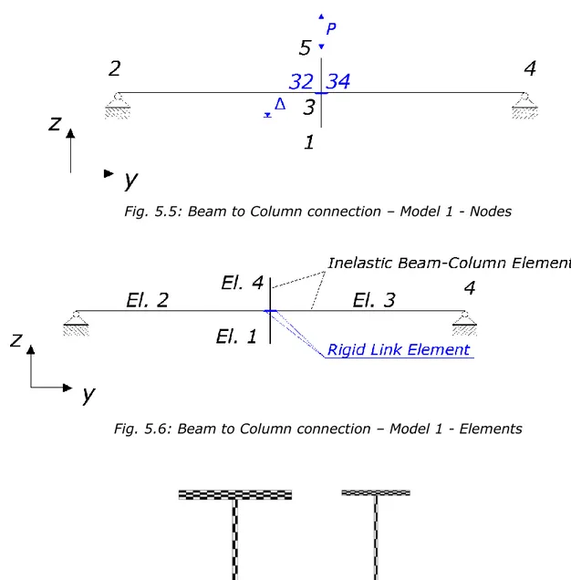
The model 1 of the beam to column connection has been realize using pre-defined Uniaxial Material Hardening. Modeled Fiber Section of the steel cross section HEB 400 and IPE 400 have been applied to Nonlinear Beam-Column elements. In order to simulate the rigid panel zone and obtain results of both beam-end of the connection, extra-nodes have been inserted (node 32 and node 34) and related to connection node (node 3) by using two Rigid Link Elements of 20 cm each one. The model is shown in the images below. The parameters required by OpenSees to the definition of the model have been:

Fig. 5.5: Beam to Column connection – Model 1 - Nodes

Fig. 5.6: Beam to Column connection – Model 1 - Elements

(4)

5.6.2 Model 2

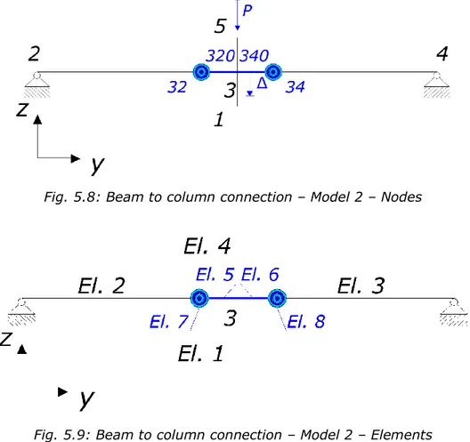
The model 2 of the Beam to column connection is realize following the “concentrated plasticity” concept. Beams and columns are modeled using pre-defined Elastic Beam-Column Element connected to Zero-Length Elements, which serve as rotational springs to represent the structure’s nonlinear behavior. The springs follow a bilinear hysteretic response based on the Modified Ibarra-Medina-Krawinkler deterioration model with bilinear hysteretic response [ref. Par. 3.9]. The input parameters for the rotational behavior of the plastic hinges are determined using empirical relationship developed by Lignos and Krawinkler in 2010 [10] which are derived from an extensive database of steel component tests. An idealized schematic of the model is presented in Fig. 5.8 and Fig 5.9, in which the spring’s side have been greatly exaggerated for clarity.

Fig. 5.8: Beam to column connection – Model 2 – Nodes

Fig. 5.9: Beam to column connection – Model 2 – Elements Where:

(5)

In this model, in order to simplify the problem, cyclic deterioration has been ignored. This was accomplished by setting:

- All the “L” deterioration parameter (basic strength, unloading stiffness, accelerated reloading, post-capping strength) to a very large number.

- All the “c” exponent variables for deterioration (basic strength, unloading stiffness, accelerated reloading stiffness, post-capping strength) equal to 1.

- Both “D” rate of cyclic deterioration variables (positive and negative loading) equal to 1.

Since a frame member is modeled as an elastic element connected in series with rotational springs at the end, the stiffness of this component must be modified so that the equivalent stiffness of this assembly is equivalent to the stiffness of the actual frame member. Based on the approach described in Appendix B of Ibarra and Krawinkler [8], the rotational springs are made “n=10” times stiffer than the rotational stiffness of the elastic element in order to avoid numerical problems and allow all damping to be assigned to the elastic element. To ensure the equivalent stiffness of the assembly is equal to the stiffness of the actual frame member, the stiffness of the elastic element must be times greater than the stiffness of the actual frame member. In this example, this is accomplished by making the elastic element’s moment of inertia times greater than the actual frame member’s moment of inertia.

In order to make the nonlinear behavior of the assembly match that of the actual frame member, the strain hardening coefficient (the ratio of post-yield stiffness to elastic stiffness) of the plastic hinge must be modified. If the strain hardening coefficient of the actual frame member is denoted and the strain hardening coefficient of the spring (or plastic hinge

region) is denoted then:

The parameters used for the definition of the backbone curve of the zero-length rotational springs have been calculated using the predefined relations provided by Krawinkler and Lignos [9] (see Par. 2.5). A Mathcad sheet has been used and the results are shown below.

(6)

The following table summarizes all the parameters requested by OpenSees for the definition of the Moment-Rotation curve used as backbone curve in the definition of the behavior of the plastic hinges.

strain hardening ratio

effective yield strength

Cyclic deterioration parameters. A large number indicates no deterioration

Rates of deterioration. 1,0 values indicate no deterioration

pre-capping rotation for positive loading direction (often noted as

plastic rotation capacity)

post-capping rotation for positive loading direction residual strength ratio for positive loading direction

ultimate rotation capacity for positive loading direction

rates of cyclic deterioration. 1,0 value indicates a symmetric hysteretic response

(7)

5.6.3 Model 2 modified

The model 2, as described in Par. 5.6.2 has been considered as a base case. Then, in order to describe the influence of deteriorating parameters on the behavior of the model, several combination of these have been considered. The same value of and the parameters have been used for all degradation (basic strength, unloading stiffness, accelerated reloading stiffness and post-capping strength) in order to simplify the number of possible combinations.

In particular six values of cyclic deterioration parameters have been taken into consideration:      

Five values of rates of deterioration parameters have been considered as well: 

   

According to that seven deteriorating models have came out, by maintaining constant one series of parameters and changing the other.

Model 2A

The changed parameters have been:

Cyclic deterioration parameters.

Rates of deterioration parameters Model 2B

(8)

Model 2C

Rates of deterioration parameters.

Model 2D

Model 2E

Model 2F

Model 2G

(9)

5.7 OpenSees Results

5.7.1 Model 1

5.7.1.1 Eigen Analysis

An Eigen analysis has been performed to check the goodness of the models. The fundamental period of the model has resulted:

5.7.1.2 Monotonic vertical force-controlled test

A monotonic vertical force-controlled test has been performed on both models. The load pattern is constituted by:

The loading ratio versus displacement diagram is shown below, where forces are conveniently represented as the ratio of the maximum applied force. The expected change of stiffness because of the occurred yield of the section, and consequently the expected loading ratio are (taking count the fact that there are two beams contemporary):

One can see the good correspondence between the expected data and the simulating test results.

Fig. 5.10: Beam to column connection - model 1 monotonic lateral load-controlled analysis 0 0.2 0.4 0.6 0.8 1 1.2 0 5 10 15 20 25 Loading Ratio F/Fmax Displacement [mm]

(10)

5.7.1.3 Reverse vertical force-controlled test

In a second moment a reverse lateral force-controlled test has been performed, to check the behavior of the model under reverse load applications. Two cycles of loading applications, with the same characteristics have been applied. The load pattern is constituted by:

Fig. 5.11: Lateral force-controlled test - loading pattern

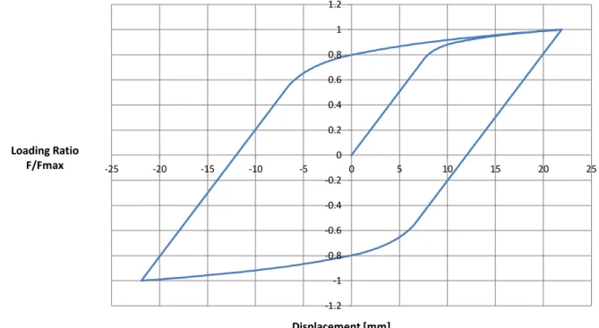
The yield loading ratio corresponds to the expected one, as shown in the previous example. In this model stiffness-and-strength degradation and pinching have not been considered. The Loading Ratio versus Displacement graphic is shown below.

Fig. 5.12: beam to column connection - model 1 reverse static lateral load-controlled analysis

-1.2 -1 -0.8 -0.6 -0.4 -0.2 0 0.2 0.4 0.6 0.8 1 1.2 -25 -20 -15 -10 -5 0 5 10 15 20 25 Loading Ratio F/Fmax Displacement [mm]

(11)

5.7.1.4 Displacement-controlled Pushover analysis

A pushover analysis has been performed on Model 1. At first a vertical load has been applied to simulate the gravity load. Then time has been reset to zero and a displacement-controlled test has been performed. The maximum displacement of the free node (node 3) has been set equal to 20% of the length of the cantilever, so 400 mm. In addiction an horizontal load has been applied to node 2:

The results of this test are presented as a Capacity curve (Base shear versus Displacement of the free node curve).

Fig. 5.13: beam to column connection - model 1 monotonic displacement controlled pushover analysis

5.7.2 Model 2

5.7.2.1 Eigen Analysis

An Eigen analysis has been performed to check the goodness of the models. The fundamental period of the model has resulted:

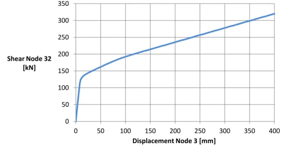
5.7.2.2 Monotonic vertical force-controlled test

A monotonic vertical force-controlled test has been performed on model 2. The load pattern is constituted by:

It’s helpful to remark that the yield moment of the spring has been increased using a factor as suggested by Krawinkler and Lignos (see Par. 2.5, [7])

The loading ratio versus displacement diagram is shown below, where forces are conveniently represented as the ratio of the maximum applied force. The expected change of stiffness because of the occurred yield of the section, and consequently the expected loading ratio are (taking count the fact that there are two beams contemporary):

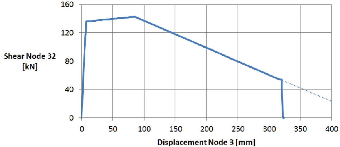
0 50 100 150 200 250 300 350 0 50 100 150 200 250 300 350 400 Shear Node 32 [kN] Displacement Node 3 [mm]

(12)

Node 3 has been chosen as displacement point, for the diagram.

One can see the good correspondence between the expected data and the simulating test results.

Fig. 5.14: Beam to column connection - model 2 monotonic lateral load-controlled analysis

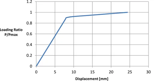
The different behavior of the first two analyzed model has been checked by putting into the same diagram the results of the monotonic load-controlled tests for model 1 and model 2. It has to be remarked that the difference of the initial stiffness of the two models derives from the modification of the stiffness of model 2, as suggested by the authors (see Par. 2.5, [7]).

Fig 5.15: Beam to column connection – monotonic load-controlled test Model 1 – Model 2 0 0.2 0.4 0.6 0.8 1 1.2 0 5 10 15 20 25 30 Loading Ratio P/Pmax Displacement [mm] 0 0.2 0.4 0.6 0.8 1 1.2 0 5 10 15 20 25 30 Loading Ratio P/Pmax Displacement [mm] Model 2 Model 1

(13)

5.7.2.3 Reverse vertical load-controlled test

In a second moment a reverse lateral force-controlled test has been performed, to check the behavior of the model under reverse load applications. Two cycles of loading applications, with the same characteristics have been applied. The load pattern is constituted by:

Fig. 5.16: Lateral force-controlled test - loading pattern

The yield loading ratio corresponds to the expected one, as shown in the previous example. In this model stiffness-and-strength degradation and pinching have not been considered. The Loading Ratio versus Displacement graphic is shown below.

Fig. 5.17: Model 2 - reverse load-controlled test

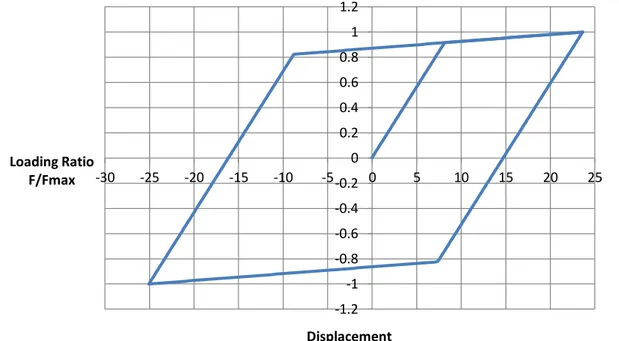
The different behavior of the first two analyzed model has been checked by putting into the same diagram the results of the reverse load-controlled tests for model 1 and model 2. It has to be remarked that the difference of the initial stiffness of the two models derives from the modification of the stiffness of model 2, as suggested by the authors (see Par. 2.5, [7]).

-1.2 -1 -0.8 -0.6 -0.4 -0.2 0 0.2 0.4 0.6 0.8 1 1.2 -30 -25 -20 -15 -10 -5 0 5 10 15 20 25 Loading Ratio F/Fmax Displacement

(14)

Fig. 5.18: Beam to column connection – reverse load-controlled test Model 1 – Model 2

5.7.2.4 Monotonic Displacement-controlled Pushover analysis

A pushover analysis has been performed on Model 3. At first self-weight loads have been applied to simulate the gravity load. Then time has been reset to zero and a displacement-controlled test has been performed. The maximum displacement of the free node (node 3) has been set equal to 20% of the length of the beams, so 400 mm. In addiction a vertical load has been applied to node 5:

Fig. 5.19: beam to column connection – Model 2 – monotonic displacement-controlled pushover analysis

One can see the shape of the backbone curve, typical for Ibarra-Medina-Krawinkler bilinear hysteretic model [7]. -1.2 -1 -0.8 -0.6 -0.4 -0.2 0 0.2 0.4 0.6 0.8 1 1.2 -30 -25 -20 -15 -10 -5 0 5 10 15 20 25 30 Loading Ratio F/Fmax Displacement Model 2 Model 1

(15)

5.7.2.5 Cyclic Displacement-controlled analysis

A cyclic displacement-controlled pushover analysis has been performed on Model 2. . At first self-weight loads have been applied to simulate the gravity load. Then time has been reset to zero and a displacement-controlled test has been performed. The imposed pattern of displacement has been based on ECCS testing procedure [18], as represented in the image below. In addiction a vertical load has been applied to node 5.

Fig. 5.20: Displacement pattern [ECCS procedure]

In the image below the shear vs displacement diagram has been represented. One can see the shape of the backbone curve and the absence of deterioration, as expected. As already specified this model has been used as a base case. In the next paragraph deterioration has been taken into account by modifying the deterioration parameters of the model.

Fig. 5.21: beam to column connection – Model 2 – cyclic displacement-controlled pushover analysis

(16)

5.7.3 Model 2 modified

5.7.3.1 Cyclic Displacement-controlled analysis

In order to describe the influence of deteriorating parameters on the behavior of the model, several cyclic displacement-controlled pushover analysis have been performed on the Model 2 modified, as defined in Par 5.6.3.

The same value of and the parameters have been used for all degradation (basic strength, unloading stiffness, accelerated reloading stiffness and post-capping strength) in order to simplify the number of possible combinations.

At first self-weight loads have been applied to simulate the gravity load. Then time has been reset to zero and a displacement-controlled test has been performed. The imposed pattern of displacement has been based on ECCS testing procedure [18], as represented in the image below. In addiction a vertical load has been applied to node 5.

Fig. 5.22: Displacement pattern [ECCS procedure]

In the next images the shear vs displacement diagrams have been represented. In all the following graphs the result of Model 2 (without deterioration) has been add as a reference, to give visual information on the rate of deterioration of the considered model.

As specified in Par. 5.6.3, the analyzed model have been:  Model 2A: constant;  Model 2B: constant;  Model 2C: constant;  Model 2D: constant;  Model 2E: constant;  Model 2F: constant;  Model 2G: constant;

(17)

Fig. 5.23: beam to column connection – Model 2A – cyclic displacement-controlled pushover analysis

(18)

Fig. 5.24: beam to column connection – Model 2B – cyclic displacement-controlled pushover analysis

(19)

Fig. 5.25: beam to column connection – Model 2C – cyclic displacement-controlled pushover analysis

(20)

Fig. 5.26: beam to column connection – Model 2D – cyclic displacement-controlled pushover analysis

(21)

Fig. 5.27: beam to column connection – Model 2E – cyclic displacement-controlled pushover analysis

(22)

Fig. 5.28: beam to column connection – Model 2F – cyclic displacement-controlled pushover analysis

(23)

Fig. 5.29: beam to column connection – Model 2G – cyclic displacement-controlled pushover analysis