Chapter 4: Analysis of a cantilever column
4.1 Abstract
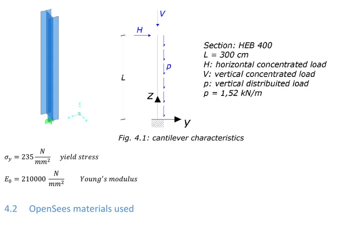
A simple cantilever column has been analyzed in order to take confidence with commands and possibilities provided by OpenSees. Plane analysis are performed in Y-Z plane (section’s strong deformation plane). The common features of the cantilever are shown below.
Fig. 4.1: cantilever characteristics
4.2 OpenSees materials used
To ensure a non linear behavior of the column only non-linear behavior material have been considered. Specifically:
Uniaxial Material Hardening
Uniaxial Material Steel01 [ref. par. 3.5] Uniaxial Material Steel02 [ref. par. 3.5]
Modified Ibarra-Medina-Krawinkler deterioration model with bilinear hysteretic response [ref. par. 3.9]
4.3 OpenSees sections used
The sections used to model the non linear behavior of the cantilever column have been: Fiber section [ref. par. 3.6]
Zero-length section [ref. par. 3.6]
4.4 OpenSees elements used
The element used to model the non linear behavior of the column have been: Elastic Element [ref. par. 3.7]
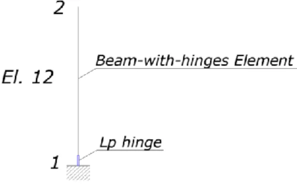
Nonlinear Beam-Column Elements [ref. par. 3.7] Beam With Hinges Elements [ref. par. 3.7]
4.5 OpenSees Models
4.5.1 Model 1
The model 1 of the cantilever column is realize using pre-defined Uniaxial Material Hardening. A modeled Fiber Section of the HEB 400 is applied to Nonlinear Beam-Column element, as shown below. The parameters added to the model have been:
4.5.2 Model 2
The model 2 of the cantilever column is realize using pre-defined Uniaxial Steel01. A Fiber section is used as before and applied to a Nonlinear Beam-Column element as shown below. The parameters added to the model have been:
Fig. 4.2: Cantilever – Model 1 ; Model2
Fig. 4.3: Fiber section discretization of the HEB400 section
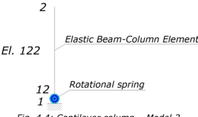
4.5.3 Model 3
The model 3 of the cantilever column is realize following the “concentrated plasticity” concept. The cantilever is modeled using a pre-defined Elastic Beam-Column Element connected to a Zero-Length Element, which serve as rotational springs to represent the structure’s nonlinear behavior. The spring follows a bilinear hysteretic response based on the Modified Ibarra-Medina-Krawinkler deterioration model with bilinear hysteretic response [ref. Par. 3.9]. The input parameters for the rotational behavior of the plastic hinges are determined using empirical relationship, derived from an extensive database of steel component tests. An
idealized schematic of the model is presented in Fig. 4.4, in which the spring’s side have been greatly exaggerated for clarity.
Fig. 4.4: Cantilever column – Model 3
In this model, in order to simplify the problem, cyclic deterioration has been ignored. This was accomplished by setting:
- All the “L” deterioration parameter (basic strength, unloading stiffness, accelerated reloading, post-capping strength) to a very large number.
- All the “c” exponent variables for deterioration (basic strength, unloading stiffness, accelerated reloading stiffness, post-capping strength) equal to 1. - Both “D” rate of cyclic deterioration variables (positive and negative loading)
equal to 1.
Since a frame member is modeled as an elastic element connected in series with rotational springs at the end, the stiffness of this component must be modified so that the equivalent stiffness of this assembly is equivalent to the stiffness of the actual frame member. Based on the approach described in Appendix B of Ibarra and Krawinkler (2005), the rotational springs are made “n=10” times stiffer than the rotational stiffness of the elastic element in order to avoid numerical problems and allow all damping to be assigned to the elastic element. To ensure the equivalent stiffness of the assembly is equal to the stiffness of the actual frame member, the stiffness of the elastic element must be times greater than the stiffness of the actual frame member. In this example, this is accomplished by making the elastic element’s moment of inertia times greater than the actual frame member’s moment of inertia.
In order to make the nonlinear behavior of the assembly match that of the actual frame member, the strain hardening coefficient (the ratio of post-yield stiffness to elastic stiffness) of the plastic hinge must be modified. If the strain hardening coefficient of the actual frame member is denoted and the strain hardening coefficient of the spring (or plastic hinge
region) is denoted then:
The parameters used for the definition of the zero-length rotational spring have been:
strain hardening ratio
effective yield strength
Cyclic deterioration parameters. A large number indicates no deterioration
Rates of deterioration. 1,0 values indicate no deterioration
pre-capping rotation for positive loading direction (often noted as plastic rotation capacity)
post-capping rotation for positive loading direction
residual strength ratio for positive loading direction
ultimate rotation capacity for positive loading direction
rates of cyclic deterioration. 1,0 value indicates a symmetric hysteretic response
4.5.4 Model 3 modified
The model 3, as described in Par. 4.5.3 has been considered as a base case. Then modifications on deteriorating parameter has been done. In particular:
Model 3A
The changed parameters have been:
Cyclic deterioration parameters. This parameter controls deterioration
Rates of deterioration. 1,0 values indicate no deterioration
Model 3B
The changed parameters have been:
Cyclic deterioration parameters. This parameter controls deterioration
Rates of deterioration. 1,0 values indicate no deterioration
Model 3C
The changed parameters have been:
Cyclic deterioration parameters. This parameter controls deterioration
Rates of deterioration. indicates deterioration
Model 3D
The changed parameters have been:
Cyclic deterioration parameters. This parameter controls deterioration
4.5.5 Model 4
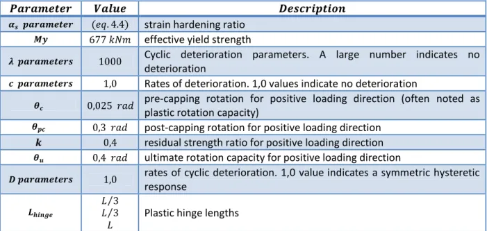
The model 4 of the cantilever column is realize following the “distributed plasticity” concept. The cantilever is modeled using a pre-defined Beam With Hinges Element. Plastic hinge regions are assigned to the ends of these elements. The plastic regions have an elastic axial response and a bilinear rotational response based on the Modified Ibarra-Medina-Krawinkler deterioration model with bilinear hysteretic response [ref. Par. 3.9]. An idealized schematic of the model is presented in Fig. 4.5. In this model, as well as the model 3, cyclic deterioration has been ignored using the same set of parameters above described.
Fig. 4.5: Cantilever column – Model 4
In this model the plasticity is distributed over a defined length. The axial and flexural responses of each plastic hinge region are defined as separate sections. The axial response is defined by an elastic section while the flexural response is defined by a uni-axial section using the bilinear material based on the Modified Ibarra-Medina-Krawinkler Model. The responses are combined into a single section using the section aggregator command. P-M interactions are neglected in this example.
In this model, as well as model 3, a stiffness modification has been performed so that the strain hardening of the plastic hinge region could capture the actual frame member’s strains hardening. In order to make the nonlinear behavior of the assembly match that of the actual frame member, the strain hardening coefficient (the ratio of post-yield stiffness to elastic stiffness) of the plastic hinge must be modified. If the strain hardening coefficient of the actual frame member is denoted and the strain hardening coefficient of the spring (or plastic hinge
region) is denoted then:
The other parameters used for the definition of the plastic section have been:
strain hardening ratio
effective yield strength
Cyclic deterioration parameters. A large number indicates no deterioration
Rates of deterioration. 1,0 values indicate no deterioration
pre-capping rotation for positive loading direction (often noted as plastic rotation capacity)
post-capping rotation for positive loading direction
residual strength ratio for positive loading direction
ultimate rotation capacity for positive loading direction
rates of cyclic deterioration. 1,0 value indicates a symmetric hysteretic response
Plastic hinge lengths
4.6 Analysis performed
4.6.1 Eigen Analysis
An Eigen analysis has been performed at first to check the goodness of the models. The fundamental period of the Opensees models has been reported
4.6.2 Monotonic lateral force-controlled test
A monotonic lateral force-controlled test has been performed on both models. The load pattern is constituted by:
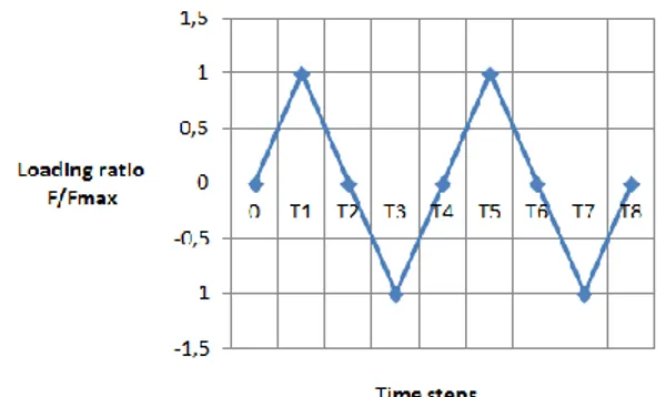
4.6.3 Reverse lateral force-controlled test
In a second moment a reverse lateral force-controlled test has been performed, to check the behavior of the model under reverse load applications. Two cycles of loading applications, with the same characteristics have been applied. The load pattern is constituted by:
Fig. 4.7: Cantilever column – Reverse lateral force-controlled analysis - Quantities
Fig. 4.8: Lateral force-controlled test - loading pattern
4.6.4 Monotonic lateral displacement-controlled pushover analysis
A monotonic pushover analysis has been performed on the pre-defined. At first a vertical load has been applied to simulate the gravity load. Then time has been reset to zero and a displacement-controlled test has been performed. The maximum displacement of the free node (node 2) has been set equal to 20% of the length of the cantilever, so 600 mm. In addiction an horizontal load has been applied to node 2:
Three values of axial force have been taken into consideration to analyze the influence of this parameter on the behavior of the model.
Fig. 4.9: Cantilever column – Monotonic lateral pushover analysis - Quantities
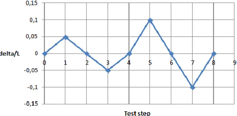
4.6..5 Cyclic displacement-controlled pushover analysis
A cyclic pushover analysis has been performed on Model 2. At first a vertical load has been applied to simulate the gravity load. Then time has been reset to zero and a displacement-controlled test has been performed. The following pattern has been applied to node 2:
Fig. 4.10: Cyclic displacement-controlled test - Displacement pattern
Three values of axial force have been taken into consideration to analyze the influence of this parameter on the behavior of the model.
4.7 Analysis results
4.7.1 Eigen Analysis
An Eigen analysis has been performed to check the goodness of the models. The fundamental period of the model has resulted:
4.7.2 Monotonic lateral force-controlled test
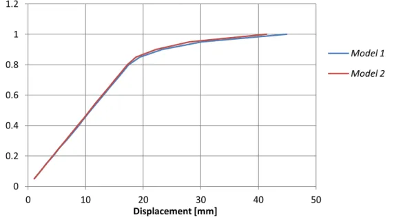
4.7.2.1 OpenSees Model 1 and Model 2The loading ratio versus displacement diagram of the first two models is shown below, where forces are conveniently represented as the ratio of the maximum applied force. The expected change of stiffness because of the occurred yield of the section, and consequently the expected loading ratio are:
One can see the good correspondence between the expected data and the simulating test results.
Fig. 4.12: Cantilever model 1-2 – monotonic lateral load-controlled analysis The two model are characterized from a very similar behavior both pre and post yielding. After that the dependence of the axial force in the behavior of the models has been checked by assign three values of the load. The three curves obtained by the analysis are shown in the next image. 0 0.2 0.4 0.6 0.8 1 1.2 0 10 20 30 40 50 Loading ratio F/Fmax Displacement [mm] Model 1 Model 2
Fig. 4.13: cantilever model 1-2 – monotonic lateral load-controlled analysis – influence of the vertical load
4.7.2.2 OpenSees Model 3
The loading ratio versus displacement diagram is shown below, where forces are conveniently represented as the ratio of the maximum applied force. The expected change of stiffness because of the occurred yield of the section, and consequently the expected loading ratio are:
One can see the good correspondence between the expected data and the simulating test results.
Fig. 4.14: Cantilever model 3 – monotonic static lateral load-controlled analysis 0 0.2 0.4 0.6 0.8 1 1.2 0 10 20 30 40 50 60 70 Loading ratio F/Fmax Displacement [mm] V=-100 kN V=-300 kN V=-500 kN 0 0.2 0.4 0.6 0.8 1 1.2 0 10 20 30 40 50 Loading ratio F/Fmax Displacement [mm] Model 1 Model 2 Model 3
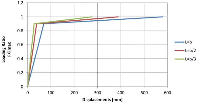
4.7.2.3 OpenSees Model 4
The loading ratio versus displacement diagram is shown below, where forces are conveniently represented as the ratio of the maximum applied force. The expected change of stiffness because of the occurred yield of the section, and consequently the expected loading ratio are:
As expected the behavior of the model is deeply influenced by the length of the plastic hinge in correspondence with the fixed node. So 3 different length have been taken into consideration:
/2 /3
Where is the cross-section depth.
The loading ratio versus displacement diagrams are shown below. One can see the good correspondence between the expected data and the simulating test results.
Fig. 4.15: Cantilever model 4 – monotonic static lateral load-controlled analysis
4.7.3 Reverse lateral force-controlled test
4.7.3.1 OpenSees Model 1 and Model 2In this case, as well as the monotonic one, the behavior of the Model1 and Model2 of the cantilever column are very similar. The yield loading ratio corresponds to the expected one, as shown in the previous example. In this model stiffness-and-strength degradation and pinching have not been considered. The Loading Ratio versus Displacement graphic is shown below.
0 0.2 0.4 0.6 0.8 1 1.2 0 100 200 300 400 500 600 Loa d in g R at io F/ Fm ax Displacements [mm] L=b L=b/2 L=b/3
Fig. 4.16: Cantilever model 1-2 – reverse static lateral load-controlled analysis
4.7.3.2 OpenSees Model 3
The Loading Ratio versus Displacement graphic is shown below. The yield loading ratio corresponds to the expected one, as shown in the previous example. In this model stiffness-and-strength degradation and pinching have not been considered.
Fig. 4.17: Cantilever model 3 – reverse static lateral load-controlled analysis 4.7.3.3 OpenSees Model 4
A reverse lateral force-controlled test has been performed on Model 4, to check the behavior of the model under reverse load applications. Two cycles of loading applications, with the same characteristics are applied. The load pattern is shown in the graphic below.
-1.5 -1 -0.5 0 0.5 1 1.5 -30 -20 -10 0 10 20 30 Loa d in g R at io F/ Fm ax Displacement [mm] Model 2 Model1 -1.5 -1 -0.5 0 0.5 1 1.5 -30 -20 -10 0 10 20 30 Loa d in g R at io F/ Fm ax Displacements Model 3
Also in this case, 3 different plastic-hinge lengths have been considered. A vertical load has been added to node 2, as axial load. In this model stiffness-and-strength degradation and pinching have not been considered. The Loading Ratio versus Displacement graphics are shown below.
Fig. 4.18: Cantilever model 4 – reverse static lateral load-controlled analysis
4.7.4 Monotonic displacement-controlled Pushover analysis
4.7.4.1 OpenSees Model 1 and Model 2
Three values of axial force have been taken into consideration to analyze the influence of this parameter on the behavior of the model. The results of this test are presented as a Capacity curve (Base shear versus Displacement of the free node curve).
Fig. 4.19: Cantilever model 2 – Capacity curve -1 -0.8 -0.6 -0.4 -0.2 0 0.2 0.4 0.6 0.8 1 -200 -150 -100 -50 0 50 100 150 200 Loa d in g R at io F/ Fm ax Displacements [mm] L=b/2 L=b/3 L=b/4 0 50 100 150 200 250 300 350 0 100 200 300 400 500 600 700 Ba se Sh e ar [ kN] Displacement [mm] Model 2 N=-1000 kN Model 2 N=-1500 kN Model2 N=-2000 kN
4.7.4.2 OpenSees Model 3
The Capacity curve (Base shear versus Displacement of the free node curve) of Model 3 is shown in the next image.
Fig. 4.20: Cantilever model 3 – Capacity curve 4.7.4.3 OpenSees Model 4
A displacement-controlled Pushover analysis has been performed on Model 4. As expected the behavior of the model is deeply influenced by the length of the plastic hinge in correspondence with the fixed node. So 3 different length have been taken into consideration:
/2
/3
Where is the cross-section depth.
Fig. 4.21: cantilever – model 4 – Displacement-controlled Pushover analysis Capacity curve 0 50 100 150 200 250 300 350 0 100 200 300 400 500 600 700 Ba se Sh e ar [ kN] Displacement [mm] Model 2 N=-1000 kN Model 3 N=-1000 kN
4.7.5 Cyclic displacement-controlled Pushover analysis
4.7.5.1 OpenSees Model 1 and Model 2Three values of axial force have been taken into consideration to analyze the influence of this parameter on the behavior of the model. The results of this test are presented as a Capacity curve (Base shear versus Displacement of the free node curve).
Fig. 4.22: Cantilever Model 2 - Cyclic displacement-controlled test – capacity curve
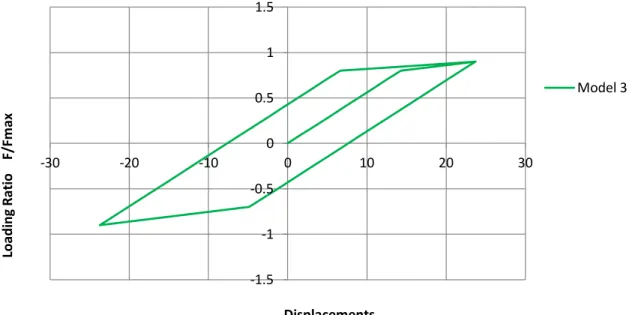
4.7.5.2 OpenSees Model 3
Fig. 4.23: Displacement pattern applied to node 2
The result of this analysis is shown in the base shear vs displacement diagram below. In this model deterioration has been neglected by setting deterioration parameters in an appropriate way, as already specified. This model has been considered as a base case.
-400 -300 -200 -100 0 100 200 300 400 -400 -300 -200 -100 0 100 200 300 400 Ba se Sh e ar [ kN] Displacement [mm] N=-2000 kN N=-1500 kN N=-1000 kN
Fig. 4.24: Cantilever – Model3 (base case) – Capacity curve
4.7.5.3 OpenSees Model 3 modified
The results of this analysis are shown in the base shear vs displacement diagrams in the next images, in which they are compared with the ones obtained by the Model 3 (base case).
Model 3 (base case) Model 3A
Model 3B Model 3C Model 3D
Fig. 4.26: Cantilever – Model 3B – Capacity curve
Fig. 4.27: Cantilever – Model 3C – Capacity curve
![Fig. 4.14: Cantilever model 3 – monotonic static lateral load-controlled analysis 0 0.2 0.4 0.6 0.8 1 1.2 0 10 20 30 40 50 60 70 Loading ratio F/Fmax Displacement [mm] V=-100 kN V=-300 kN V=-500 kN 0 0.2 0.4 0.6 0.8 1 1.2 0 10 20 30 40 50 Loading ratio F/](https://thumb-eu.123doks.com/thumbv2/123dokorg/7630968.117255/10.893.198.819.783.1103/cantilever-monotonic-lateral-controlled-analysis-loading-displacement-loading.webp)