II – DESCRIPTION OF PHENOMENA
II.1 – The reaction of water recombination; II.2 – ACP-PCP interface; II.3 – The porous structure of the central membrane; II.4 – Charge transport; II.5 – Transport in gas phase; II.6 – Water transport in PCP; II.7 – Towards the model of the central membrane; II.8 – Proof of the concept and experimental set up; II.9 – References.
II.1 – The reaction of water recombination
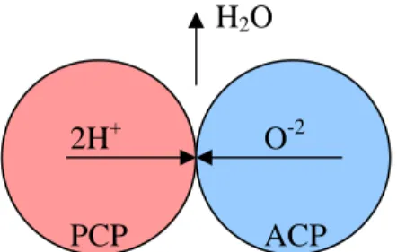
The main process that happens in the central membrane is the reaction between protons (H+), coming from the anodic side, and oxygen ions (O-2), coming from the cathodic side, to produce water. Protons are transported by a proton-conducting phase (PCP), oxygen ions by an anion-conducting phase (ACP), water produced goes into the gas phase (fig. II.1). Note that we are assuming in first instance that there is no-mixed conduction, i.e. each species is transported and belongs only at its respective phase, so there is not any oxygen or water transport into PCP, protons or water transport in ACP and protons or oxygen transport in gas phase. This is not a strong assumption at this moment1, it is based on the consideration that the global reaction is:
2 (g) 2 ) ACP ( ) PCP ( O H O H 2 + + − (reac. II.1.1)
so protons are initially in the PCP, oxygen ions in ACP and finally water is placed into the gas phase; we do not consider now the kinetic mechanism, we just watch at the overall reaction.
fig. II.1 – Overall mechanism of water recombination.
1 We will see in par. II.6 that, due to the nature of the PCP used (in particular barium cerate doped with
yttria, BCY), there is a partial transport of water inside the PCP; we will still assume no transport of protons in ACP or of oxygen ions in PCP (neglecting in this way the mixed conduction) and, obviously, the transports of H+ and O-2 into gas phase.
2H+ O-2
H2O
According to (reac. II.1.1), the reaction will take place where reagents and product may coexist together. This happens at the three phase boundary (TPB) among PCP, ACP and gas phase. The TPB is the monodimensional region that separates one phase from the others. For example if particles are overlapping spheres TPB is the circumference that surrounds the circular contact area between ACP and PCP. It is clearly an idealization: reaction will happen actually in a finite volume close to the geometric TPB, as in a surface reaction the kinetic process involves a finite depth (even if very small if compared with other two dimensions). In theory, reaction may occur at the interface between ACP and PCP (i.e. not in contact with gas phase) if water transport inside one of these phases is possible.
In the following, we assume that the global reaction takes place at the TPB and we will refer all kinetic parameters at this monodimensional length. It is essentially due to the fact that we will consider a macro-kinetics, i.e. a kinetics referred to the overall reaction as written in (reac. II.1.1); in this way, considering that we do not know anything in particular on the reaction, kinetics referred to the length of the TPB is more coherent according to the fact that (reac. II.1.1) involves three phases in the global. We will never talk about elementary mechanisms that could happen for example only at the ACP-PCP interface2. To write a mechanism of the reaction (i.e. a sequence of elementary steps) an accurate study on materials and specific experiments are needed3; at this state of the art it is difficult to perform them and they have a secondary importance compared with the understanding and the description of all the phenomena, not only of the water recombination kinetics.
Note that (reac. II.1.1) is reversible, i.e. it can occur in a direction or in the other one according to the conditions relative to equilibrium. When the fuel cell works as an energy supplier, water production is expected (even if, due to local equilibrium effects, in some points of the CM reaction could proceed in the other direction); on the other hand, (reac. II.1.1) proceeds from right to left if the system is forced to split water into hydrogen and oxygen (it is possible by applying a difference of potential at cathode and
2
Imagine that (reac. II.1.1) occurs in two steps: in the first one protons and oxygen ions react together at the ACP-PCP interface to produce water in PCP, the second step is the transport of water to the gas phase through PCP. Depending on which one is the rate determining step, the overall rate of reaction could be proportional to the contact area between ACP-PCP (if step 1 is slow and water transport in PCP is quick) or not (if water transport in PCP is slow, it forces the reaction to occur in a small region close to the TPB and in this case the global rate is proportional to the length of TPB).
3 To have an idea on micro-kinetics models applied to SOFCs, see for example Bessler (2005) or Bieberle
and Gauckler (2002). It is possible to use this kind of approach if the system is “mature”, i.e. if there is an accurate knowledge of properties of materials and if mechanisms have been demonstrated to be experimentally coupled with specific measurements of kinetic parameters for each step.
anode bigger than OCV and opposite to it, so able to change the global direction of the current inside the cell). We could see the reaction in terms of current: when water is produced, the current (assumed made of ideal positive charges) flows from PCP to ACP, in the other case current flows from ACP to PCP4. So, when water is produced we talk about an exchange of current from PCP to ACP, when water is consumed an exchange from ACP to PCP.
II.2 – ACP-PCP interface
To talk about kinetic expressions and to describe dynamic effects concerning the water recombination reaction, a coherent model of the behaviour of the ACP-PCP interface, based on the physical description of it, is needed.
According to the description of the reaction as explained in the previous paragraph, the interface between ACP and PCP and its behaviour have a central role in the understanding of the central membrane. We can imagine that ACP and PCP are separated by a bidimensional interface (i.e. a surface in the mathematical meaning): on one side there is the ACP, on the other side the PCP and in the middle the interface. On the other hand, we could think at this interface as a diffuse layer, i.e. we could imagine that properties change with continuity from ACP to PCP in a very small thickness that we call interface. Anyway, the interface separates the bulks of the two phases5. In the following we will represent the ACP-PCP interface in the first way, i.e. with the mathematical meaning of bidimensional (not diffused) interface. It is not an arbitrary interpretation of the reality, it is only a model of behaviour that suits with our general approach explained above, i.e. to describe the reaction with a macro-kinetics and to write mass and charge balances and transports according to this model6.
4
Note that when oxygen ions go from the bulk of ACP towards the TPB, it is as the current flowed from TPB to the bulk of ACP and vice versa. This is due to the fact that oxygen ions are negatively charged, current is always assumed as a flux of positive charges.
5 It is similar to the definition, for example, of solid-gas interface: especially for the gas phase, we can
think that properties change with continuity from the wall to the bulk or we can imagine to converge these phenomena into a small layer that we represent as a bidimensional interface. These are two different models to describe the contact between solid and gas; there is not a correct or a wrong one: we must be coherent with the description adopted by using appropriate equations.
6
It is clear that it is impossible (or, at least, quite difficult) to describe a phenomenon without an idealization of its behaviour, especially in our case, i.e. in an innovative field. Thus, in whole chap. II we try to describe the phenomena as much objective as we can, but it is clear that there is always an idealization of the phenomenon, i.e. a simple model of the elementary behaviour. For example, describing the ACP-PCP interface we have idealized the interface and described this idealization. Anyway, we have tried to show all these hidden assumptions when it has been possible.
A difference of potential is expected to exist between ACP and PCP. We have already said that the natural tendency of the global cell reaction is to convert hydrogen and oxygen into water because the standard Gibbs free energy is less than zero (par. I.2); because the cell reaction is composed by semi-reactions at cathode, anode and CM, these semi-reactions reflect the same behaviour of the global one.
Imagine ACP and PCP as in fig. II.1 surrounded by a dry atmosphere, initially the two phases are electrically neutral. Now, the thermodynamic tendency of the system is to combine H+ and O-2 to create water, so protons and oxygen ions react and water is produced. This leads to the disappearance of positive charges in PCP (i.e. it tends to become negatively charged) and of negative charges in ACP (i.e. it tends to become positively charged): in this way, a difference of potential VACP – VPCP > 0 is created. As the reaction proceeds, assuming for instance that the system is closed, the difficulty of reagents to react increases because they have to win a difference of potential opposing the reaction: if we imagine that in the mechanism of reaction protons jump on ACP to form adsorbed water, they are positive charges that have to go from a negative to a positive phase; if we suppose that oxygen ions spill on PCP to form water, they are negative charges that have to go from a positive to a negative phase: in both cases, the difference of potential between ACP and PCP is a contrary force for the water recombination. Then, also the water produced can split into protons and oxygen ions (i.e. (reac. II.1.1) can flow also from right to left) and the rate of reverse reaction increases as the concentration of water in gas phase increases.
We can imagine that the system will arrive at an equilibrium in which the difference of potential between phases and the partial pressure of water are enough to balance the chemical affinity of H+ and O-2; we could expect that the difference of potential increases if the “concentrations” of reagents increase and of product decreases and vice versa, i.e. according to the Nernst law for electrochemical equilibrium. We know that this representation is only a simple schematic idealization of the reality, but it explains the genesis of the difference of potential between ACP and PCP. More appropriate and accurate explanations could be given to describe this phenomenon, we have chosen this way according to its simplicity and because it agrees with our way of looking at the system (i.e. the way of chemical engineering).
Now we can eliminate the initial hypothesis of closed system (useful only for an easy visualization of the concepts described): if reagents H+ and O-2 are supplied with continuity (it happens by supplying molecular hydrogen and oxygen to electrodes) and
water is evacuated in the same manner, the system will work in the same way, so a difference of potential between ACP and PCP is created with VAPC > VPCP7. Protons and oxygen ions reach the TPB by migration (see par. II.4) where they react to form water that is carried away from the reaction site by the gas phase.
It shall be noted that this model of behaviour of the ACP-PCP interface leads to draw some conclusions:
1. we are assuming that the system follows the electrochemical laws of equilibrium (i.e. Nernst law);
2. the difference of potential between ACP and PCP affects the kinetics (i.e. the rate of water production) because it is a contribution of energy that we can sum to the thermal activation energies of direct and reverse reactions;
3. the charge/discharge of phases shall lead to a capacitive behaviour of the interface.
As far point 1 is concerned, it shall be noted that it is not immediate that the reaction of water recombination should follow the laws of electrochemical reactions because there are not free electrons involved as it happens at electrodes. Protons and oxygen ions can be seen as chemical species, so they could follow the law of chemical equilibrium, to make an example close to chemical engineering, the same law that describes the reaction of ammonia formation starting from nitrogen and hydrogen. The principal difference between water recombination inside the CM and the ammonia formation is related to the charge of species: in the formation of ammonia reagents and product are neutral, in (reac. II.1.1) reagents have a charge. These charges lead these species to behave in a different way, in particular they will also be submitted to electric forces due to this feature (electric fields have effects only on charged species). In other words, we may say that we must treat water recombination reaction following electrochemical laws according to the fact that species are charged8.
Point 2 is very important because it implies that the difference of potential between ACP and PCP affects the rate of water recombination. In particular, with other working conditions fixed, the value of VACP – VPCP compared to the same difference calculated
7
Note that, in a similar way, the potential of the cathode is higher than the potential of the anode, the genesis is the same.
8 Chemistry and electrochemistry are not separated sciences: the first one deals with neutral species, the
second one with charged species (i.e. when electric field affects the reactions). Note that in electrochemistry chemical laws are still valid; in other words, we could say that electrochemistry is an extension of chemistry in which electric effects are considered together with chemical effects.
↑ V
∆
at the equilibrium9 determines the rate of reaction. We call this entity overpotential (
η
): when VACP – VPCP is lower than (VACP – VPCP)eq (i.e.η
> 0) it is easier for protons and oxygen ions to react because the spillover of charged species meets a lower resistance, so (reac. II.1.1) flows preferentially from left to right; in the other case (i.e.η
< 0) water split occurs. But we are saying more: the value of the overpotential settles not only the direction of the reaction (i.e. thermodynamic effect) but also its rate (i.e. kinetic effect): the rate of water formation will be high if the overpotential is high and vice versa. This is due to the fact the direct and reverse reactions have to win a resistance to happen, we usually call these resistances activation energies. In an electrochemical system, activation energies are made of a thermal-chemical component (due to the chemical affinity of species and to the way that reaction follows) and an electric component, i.e. a contribution related to the interactions between electric field and charged species. In our case, it is straightforward to imagine that ifη
> 0 (i.e. phases have a difference of potential lower than at equilibrium) charged reagents will have a lower energy barrier to win, so the direct reaction will go faster and vice versa. Thus, we expect that the kinetic law will depend on overpotential.It is not difficult to understand conclusion 3: if there is a difference of potential between ACP and PCP, we can imagine that the interface behaves in a way similar to an electric condenser. When phases are charged or discharged there will be relative currents to allow these processes, we could idealize this situation by using the theoretical capacitive behaviour of a condenser: when current is supplied to the positive side and subtracted from the negative one, the difference of potential between the sides increases and vice versa (fig. II.2).
fig. II.2 – Scheme of an ideal electric condenser.
All these considerations are not theoretical extrapolations, the behaviour described has been experimentally observed (e.g. dependence of overpotential on the kinetics of water
9
The value VACP – VPCP at the equilibrium is quite similar to the definition of OCV for the whole cell,
they have the same meaning.
+ + + + + + + - - - - - - - i i
formation, capacitive behaviour, Thorel et al., 2009) even if not at this micro-scale, but it is demonstrated that the cell and the central membrane show these features.
II.3 – The porous structure of the central membrane
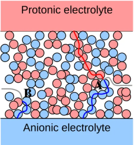
Until now we have talked about the reaction and the interface from a micro-scale point of view, i.e. we have considered only a contact between ACP and PCP. But it is easy to understand that a single contact is not enough to have high performances (i.e. high rates of water formation): if we had only a contact it would be impossible to reach high current exchanged. Due to this reason, as already mentioned in chap. I, the central membrane is a porous composite layer of ACP and PCP particles; in this way, there are several contacts between ACP and PCP (i.e. several TPBs) where reaction may occur.
Let us watch again fig. II.1: to have steady-state conditions as required for a stable production of current, reagents must be supplied and water must be carried away with continuity; if one of these three phenomena is not guaranteed (i.e. it is impossible to supply protons or oxygen ions or to carry away water) the reaction stops. Remember that protons come from the anode through the protonic electrolyte, oxygen ions from the cathode through the anionic electrolyte and water is discharged into the atmosphere outside of the CM. So, there are 3 different paths: one that supplies protons from dense protonic electrolyte towards TPB, a similar one made of ACP for the transport of oxygen ions, and one for water into the gas phase (i.e. within the pores) that links TPB with the external atmosphere. All these paths must be connected to their relative sources of reagents (i.e. the two dense electrolytes at the lateral sides of the CM) or sink of product (i.e. the external atmosphere).
These concepts are schematically shown in fig. II.3 in two dimensions. PCP is represented in pink, ACP in light blue, gas phase is white; paths have a darker colour (red for the path of protons, blue for oxygen ions and grey for water in gas phase). Paths can be covered in one direction (i.e. from electrolytes to TPB and then to external atmosphere: water production) or in the other one (i.e. water flows from atmosphere to TPB and charges come back to electrolytes: water consumption). In A the TPB is potentially active for the reaction because all the paths are connected; in B it is impossible that reaction happens because in this point PCP is not connected with its source of protons (i.e. the protonic electrolyte).
fig. II.3 – 2D representation of the porous composite structure of the CM with the 3 different paths.
We have just seen that not the whole TPB is active, only the connected fraction of the total TPB is available for the reaction. In the following, when we will talk about TPB, we will always refer to the active TPB (i.e. with the acronym TPB we will refer only to the active three phase boundary). It is clear that it is important to maximize the total length of the TPB to reach high current exchange. For this reason a porous composite membrane is used instead of the simple contact between the two electrolytes. In conclusion, the total length of TPB is a morphological parameter strictly linked to the reaction rate, i.e. the total flux of water produced will be high if the total length of TPB is high or the kinetics is fast.
But it is simple to understand that the extension of the boundary where reaction may occur is not the only parameter that affects the global reaction rate. If we imagine a situation in which the reaction is very quick, the bottle neck could be represented by the transport of reagents or product. In other words, if reaction is quick, the global rate of water production will be determined by the slowest step, i.e. the transport of one of the species. For example, if the transport of protons is slow compared to other transports and the intrinsic rate of the reaction, the rate of the water production will be at maximum equal to the rate of the supply of protons; if the transport of oxygen was the slowest phenomenon, the scenario would be the same. The global rate could be limited also by the rate of water evacuation: if it is difficult to carry away water from the porous structure, at the TPB the reaction will be at a local quasi-equilibrium, occurring at the same rate of the transfer of water. Thus, also the resistances of transport shall be considered and these resistances are connected with the morphological properties of the
Protonic electrolyte
Anionic electrolyte
A
B
CM (e.g. the length and the total number of paths) and intrinsic properties of phases (e.g. conductivities of ACP and PCP, diffusivity of water in gas phase).
It is evident that the length of TPB and the resistances of transport depend strongly on the morphology of the CM, in particular we can make this distinction:
• the total length of TPB will be proportional to the total number of contacts between anion-conducting particles and proton-conducting particles and it also depends on the fraction of connected paths;
• rates of transports will be high if an high number of paths of the same type is guaranteed (e.g. if there are several contacts ACP-ACP the conduction of oxygen ions will be easier).
Now, the two aims of increasing the reaction sites and the rates of transfer are partly incompatible. To maximize the length of TPB a high number of ACP-PCP contacts is needed while to maximize transport we need to increase the contacts of particles of the same type or the porosity. Generally speaking, a compromise shall be reached; then, it is reasonable that the best design of the CM should increase the total length of TPB if the kinetics is the rate determining step, on the other hand we should help the transport of the reagent or product that is too slow.
Concluding, we must consider that the morphology of the central membrane has a strong influence on its performances, so it is necessary an accurate description of it to evaluate the functional parameters (i.e. length of TPB, ohmic conductivities of solid phases and transport properties of gas phase). In chap. III we will develop a mathematical model for the estimation of these parameters.
II.4 – Charge transport
In the description of ACP-PCP interface (par. II.2) we said that charges (i.e. protons and oxygen ions) are transported by migration. This kind of transport, in which the flux of charges is due to an electric field (i.e. a gradient of electric potential), is typical of solid conductors: charges have to spend energy to move through the solid phase, so electric potential decreases in the direction of the current flow. In other words, the Ohm law is assumed to describe charge transport for both protons in PCP and oxygen anions in ACP.
More details will be given in par. IV.4 where also the justification of this assumption will become clearer.
II.5 – Transport in gas phase
Concerning the gas phase, we shall remember that its domain is constituted by the pores of the structure. Then, not only water will be present in the pores, other gaseous inert species will be present in relation with the composition of the external atmosphere: if a flow of nitrogen is used out of the cell to carry away the water as in experimental set up (see par. II.8 and Thorel et al., 2009), we shall also consider that nitrogen counter-diffuses inside the pores; when the cell will be ready for the market, the external atmosphere could be represented by air (assuming the compatibility of materials with oxygen, carbon dioxide and other pollutants present in air). Anyhow, at least a second component into the gas phase must be considered, in the following we will use the letter B to refer to this gaseous inert.
Imagine the CM working in the direction of water production: in some points of the porous structure there is the appearance of gaseous water. It is reasonable that this production yields two effects on the gas phase:
• the pressure inside the CM will increase;
• the molar fraction of water into gas phase will be higher in the proximity of the active sites where it is produced.
In other words, we expect the formation of gradients for both pressure and molar fraction. The first phenomenon is due to the fact that the net transport inside a porous structure is submitted to frictions. To win the resistances to the mass flow a gradient of pressure is needed. Gradients of molar fraction are due to the formation of water while there is not any production of the second component (e.g. nitrogen). It means that we shall be able to represent fluxes of water and inert according to a double driving force, i.e. a gradient of pressure and a gradient of concentration: the first one leads to a net non-separative10 flow, the second one leads to restore the uniformity of concentrations.
Moreover, if the pores are small if compared with the mean free path of the gases (i.e. the mean distance that a molecule covers between a collision with another molecule and another collision), the gas phase can not be considered as a continuum. We shall then take into account also molecule-wall collisions that introduce other terms compared to ordinary diffusion (due to gradients of concentration) and viscous flow (due to gradients of pressure). This situation is called Knudsen region (a transition region is usually considered between continuum and Knudsen region).
10 The word non-separative means that the viscous part of the flow, due to the gradient of pressure, does
not affect the composition of gas phase (i.e. it does not change the molar fractions) as explained by Kast and Hohenthanner (2000).
We have only shown a qualitative interpretation of phenomena occurring into the gas phase with the only purpose to introduce the problem; a comprehensive quantitative description will be done in par. IV.2.
II.6 – Water transport in PCP
In par. II.1 we said that we excluded mixed conductions revealing that it was not a very strong assumption and that in the following we will have considered the possibility of water transport in solid phases.
It is known that proton-conducting materials based on perovskite-structure (as used for the CM like yttria doped barium cerate) allow the transfer of water in solid phase (Kreuer, 2003; Coors, 2007); we mean that water can be adsorbed in a point of the PCP in contact with gas phase, transferred with a bulk-transport within and through the solid phase, and then desorbed in another point at the PCP-gas phase interface. ACP does not show this kind of behaviour.
It is important to understand that the water transfer in PCP is not a surface-transport, i.e. confined at the interface between PCP and gas phase, but it is a bulk-transport inside PCP; at the PCP-gas phase interface there is the adsorption/desorption of gaseous water to form protonic defects (Kreuer, 2003), i.e. water in adsorbed form in the solid phase. These protonic defects affect the effective conductivity of PCP that increases if protonic defects increase (i.e. adsorbed water helps the conduction of protons in PCP).
Several authors (Coors, 2007; Suksamai and Metcalfe, 2007) found this behaviour that we can now resume with this example. Imagine a compact layer of PCP, i.e. without porosity, and put it between two atmospheres with different partial pressures of water, pw,1 and pw,2 with pw,1 > pw,2, as in fig.II.4: we will see a flow of water from left to right, i.e. water adsorbed from one side, transported through the bulk of PCP and desorbed at the other side.
fig. II.4 – Example of water transport in PCP (pw,1 > pw,2). PCP
Thus, there is a net flow of water and the driving force is the difference of its partial pressure in gas phase: flow increases if the difference pw,1 - pw,2 increases. It is easy to imagine that the rate of water adsorption at the left side will increase if pw,1 increases. On the other hand the desorption on the right side will be faster as pw,2 decreases. Between these surface phenomena, the transport of water adsorbed in PCP will increase as the difference of the driving force increases.
We do not want to enter in details here, we just want to describe the phenomenon; a comprehensive explanation of the mechanisms11 will be performed in par. IV.3 coupled with a consistent mathematical expression of the water transport.
II.7 – Towards the model of the central membrane
The model of the CM is made of charge and mass balances, i.e. an equation of conservation is used for each species. The general balance equation, expressed per unit volume, is: v j j j P N g t C + ⋅ −∇ = ∂ ∂
φ
(eq. II.7.1)in which j is the name of the species (e.g. protons, oxygen ions, water in gas phase, etc.) and P is the phase where the species exists (i.e. ACP, PCP or gas phase). Cj is the molar concentration of j in the phase, Nj its molar flux, gjv is the generation term (i.e. the rate
of generation of j in phase P per unit volume) and φP the volume fraction of phase P referred to the whole volume of the CM. Note that generation term considers the global rate of generation of j in phase P due to reactions or to exchanges with other phases (e.g. adsorption of water in PCP), i.e. gjv can be exploded in each term of generation.
The expressions of fluxes and generation terms come from the mathematical description of the phenomena occurring in the CM, i.e. from the submodels of description of each elementary process (e.g. submodel of gas transport, submodel of charge transport, submodel of water recombination kinetics, etc.). In the previous paragraphs we have qualitatively described these phenomena that represent real features of materials (e.g. water transport in PCP) or of the system in general (e.g. porous
11 We talked here about protonic defects and water in adsorbed form: in par. IV.3 the link between them
will be shown. Now it is important to familiarize with the phenomenon, even if without its detailed physical description that could be misleading at this moment.
structure). In the following two chapters we will enter in the details of the physical representation of each phenomenon (i.e. the consistent idealization of the behaviour) coupled with its mathematical description (i.e. the quantitative relationship).
Chap. III is entirely dedicated to the description of the morphology in order to estimate the functional morphological parameters that we need in the model of the CM in chap. V: the outcomes of chap. III will be input parameters in chap. V. Several authors (Chen et al., 2009; Janardhanan et al., 2008; Kenney et al., 2009) have already tried to estimate such parameters for similar cases (i.e. electrodes of SOFCs) by using more or less the same tools that we will use (i.e. percolation theory and 3D simulations). We want to show our approach that differs in some elements from the existing models; it is structured as a general model, i.e. it can be applied to different structures (e.g. CM but also electrodes of SOFCs in general).
In chap. IV we will present the submodels for the mathematical description of the phenomena presented in this chapter (i.e. from par. II.1 to II.6 excluded II.3). In particular, we will present kinetic laws (e.g. the kinetics of the water recombination, the kinetics of water adsorption in PCP) and basic transport expressions (e.g. transport in gas phase) coherent with the physical description that we will do to the phenomenon. These submodels will enter in the model of the CM as constitutive laws giving the expressions of fluxes (i.e. Nj) and source terms (i.e. gjv).
Due to this kind of approach, that uses balance equations in which each term comes from a specific submodel, our model is therefore mechanistic and not a representation of the CM by an equivalent circuit. A model based on an equivalent circuit has limits concerning the association between physical elements of the system with basic components of the circuit. This kind of problem does not exist by using our physical approach.
It is important to emphasize that the model uses apparent properties, i.e. we model the CM as a continuum even if it is a composite material with three different phases. In this approach, fluxes Nj are referred to nominal surfaces (i.e. the geometric surface composed by the ideal section of ACP, PCP and gas phase) while the values of potential quantities that represent the driving forces12 (electric potentials, pressure, concentrations of substances inside the phases) are the effective ones that we could measure in each
12 The general idea that we follow is this: each flux (i.e. current, mass flow) is determined by the gradient
of the relative potential quantity (e.g. electric potential for current, concentration for diffusive flow, temperature for heat flow, etc.; also combined potential quantities can be considered, for example electric potential and concentration for the flow of charged species in solution) that represents the driving force. We have just done some examples for clarity.
relative phase. Let us make a simple example to clarify the concepts by using conduction in ACP. In a pure dense anion-conducting material, the Ohm law is written as:
ACP ACP
ACP V
i =−
σ
∇ (eq. II.7.2)in which VACP is the electric potential, iACP the density of current (i.e. the flux of charges) and σACP is the conductivity of the material. In a porous composite system such as the CM, if we want to model the system as a continuum, apparent properties must be used; in particular, (eq. II.7.2) becomes:
ACP app ACP
ACP V
i =−σ ∇ (eq. II.7.3)
in which VACP is still the electric potential on ACP (i.e. the real electric potential that we could measure in each point of the ACP), iACP is the density of current referred to
nominal surface and σACPapp the apparent conductivity of ACP (i.e. the proportional factor between the gradient of electric potential and density of current). Note that iACP is not the effective density of current that flows in anionic paths, it is an apparent value referred to the geometric surface of the whole porous media; the effective density of current that flows in anionic paths will be higher. Apparent conductivity depends obviously on the conductivity of the material (i.e. σACP) but also and mainly on the morphology of the CM (i.e. composition, radii of particles, angles of contact, etc.).
The use of this approach is also evident in the form of (eq. II.7.1) that is referred per unit of whole volume. So, φP is used to transform the concentration in a concentration per unit of whole volume, Nj is a flux referred to nominal surface and gjv is referred per unit of whole volume. The alternative way to work could be to distinguish the three domains, i.e. ACP, PCP and gas phase, and to write balances and transports for each phase with exchange terms between a phase and another one. This approach, closer to the reality, needs the exact knowledge of the distribution of phases inside the membrane.
This approach, i.e. the use of apparent properties, is used for the mathematical description of all transports, i.e. charge transport, gas transport and transport of water in PCP. So, all the properties that we need for the characterization of the system are apparent properties, for example apparent electric conductivities of solid phases or
apparent diffusivity in gas phase. Chap. III is dedicated to the estimation of apparent properties. In chap. IV we will get constitutive laws, then in par. V.4 we will refer them to the system by converting properties into apparent properties.
II.8 – Proof of the concept and experimental set up
It is important now to come back to the reality of the system and to talk about the experimental set up in order to have a concrete visualization of the device and to understand the inputs that we can supply (i.e. the variations from the initial condition) and the outputs that the system yields (i.e. in particular the performance indexes).
First of all, as already mentioned in par. I.3, it is important to emphasize that the IDEAL-Cell concept has been proved experimentally (Thorel et al., 2009), i.e. it has been demonstrated that the cell gives a stable open circuit voltage when reagents are supplied with continuity at the electrodes and that water is produced in the central membrane when cell is working as an energy supplier (i.e. when current flows from cathode to anode in the external circuit). So, all the efforts concerning the modelling of the system and improvements in materials and their preparations are justified by the fact that the concept has been proved.
The experimental set up used for the proof of the concept and also to obtain other experimental results is schematically reproduced in fig. II.5. A detailed description of the experimental set up can be found in Thorel et al. (2009). In few words, the cylindrical cell (made by a porous composite anode, a dense protonic electrolyte, a porous central membrane, a dense anionic electrolyte and a porous composite cathode; also metallic electrodes like platinum can be used instead of porous electrodes) is put inside a cylindrical heater that guarantees uniform temperature. The system is fed by wet hydrogen (normally about 3% of water in H2)13 at the anodic side and by dry oxygen at the cathodic side (we could also use a mixture of nitrogen and oxygen to simulate air); nitrogen (or wet nitrogen if we want) is used in the third chamber that surrounds the cell to carry away the water produced. These gases are fed by using ceramic pipes. The three compartments are isolated one from others, gaskets are used between pipes and electrolytes to avoid leakages14.
13 Hydrogen is wet to increase the conductivity of PCP (also present in cathode that is a porous composite
of PCP and electron-conducting phase) as mentioned in par. II.6.
14
Note that electrodes have a smaller diameter than electrolytes and CM, this feature makes simpler the isolation of the three chambers.
fig. II.5 – Schematic representation of the experimental set up.
We can perform several measurements with this configuration by varying several working conditions (e.g. temperature, pressure of gases and their composition, difference of potential applied to terminals) and measuring some outputs (e.g. current, humidity of nitrogen15, difference of potential if not imposed). First of all, it is possible to measure the open circuit voltage (OCV), i.e. the difference of electric potential between the terminals of the cell, that is a measurement at equilibrium.
By applying an external difference of potential different from OCV (i.e. an overpotential) and closing the external circuit, we can measure the current that passes through the cell; it is equivalent if we impose a current to pass and measure the difference of potential between cathode and anode. Usually, these results are plotted as current vs difference of potential applied or as current vs overpotential. These curves are called polarization curves and show how the system behaves at different loads (i.e. power supplied/consumed) at the steady-state.
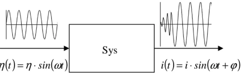
Also dynamic measurements can be performed; in the most important one a sinusoidal overpotential (or a sinusoidal current)16 is applied to the cell and current (or overpotential) is measured in the time domain at different frequencies. Usually results
15
In particular, by the measure of the humidity of nitrogen, it has been proved that water is produced in the CM and not at electrodes.
16
We mean that we impose an input as η =ηst +ηam⋅sin
(
2πf ⋅t)
where ηst is the time-invariantcontribution of overpotential, ηam is the amplitude of oscillation and f is frequency of oscillation (often
the pulsation ω = 2πf is used); to impose a current just change η with i. We will always set ηst (or ist)
equal to zero in the following.
H2
are reported in Nyquist plots as imaginary component vs real component of the impedance at several frequencies; these are called impedance curves. The impedance Z is the complex number that results from the ratio of the phasor of potential (or overpotential) and the phasor of current. The calculus of the phasor ā of a generic sinusoidal quantity g(t) is:
( )
(
ω ϕ)
(
ϕ ϕ)
jϕ e G sin j cos G g t sin G tg = ⋅ + ⇒ & = ⋅ + = ⋅ (eq. II.8.1)
where G is the amplitude of the oscillation, ω its pulsation, ϕ the phase and j the imaginary unit; in our case, phasors of current and overpotential are calculated in this way. It is possible to demonstrate that if an oscillating input is imposed (for example
( )
tη
sin( )
ω
tη
= ⋅ ) a stable physical system as the cell yields an oscillating output (for example a current i( )
t =i⋅sin(
ω
t+ϕ
)
) with the same frequency after a first transition period (fig. II.6).
η
( )
t =η
⋅sin( )
ω
t i( )
t =i⋅sin(
ω
t+ϕ
)
fig. II.6 – Schematic representation of the output i(t) of a real system when a sinusoidal input η(t) is imposed.
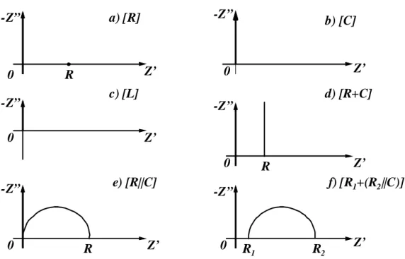
Some impedance curves of several electric circuits are reported in fig. II.7 as examples (Z’ is the real component of impedance and Z’’ the imaginary component). In the figure, R means resistance, C capacitance and L inductance; the symbol + means that the elements are in series, | | in parallel.
Impedance curves are very useful tools because they show also dynamic information, i.e. the response of the system in transient conditions; in this way, impedance curves represent the steady-state and also the dynamic behaviour of the system giving us a complete scenario17.
17 Just to make some examples, at high frequency fast processes (e.g. charge/discharge of double layer,
see par. II.2) characterize the response, at low frequency the signal is affected by slow phenomena (e.g. diffusion in gas phase).
a) [R] c) [L] e) [R||C] f) [R1+(R2||C)] b) [C] d) [R+C] Z’ Z’ Z’ Z’ Z’ Z’ -Z” -Z” -Z” -Z” -Z” -Z” R R R R1 R2 0 0 0 0 0 0
fig. II.7 – Nyquist plots (i.e. impedance curves) of elementary circuits.
II.9 – References
Bessler W.G., “A new computational approach for SOFC impedance from detailed
electrochemical reaction-diffusion models”, Solid State Ionics, 176, pp. 997-1011; 2005.
Bieberle A., Gauckler L.J., “State-space modeling of the anodic SOFC system Ni, H 2-H2O|YSZ”, Solid State Ionics, 146, pp. 23-41; 2002.
Chen D., Lin Z., Zhu H., Kee R.J., “Percolation theory to predict effective properties of
solid oxide fuel-cell composite electrodes”, J. Power Sources, 191, pp. 240-252; 2009. Coors W.G., “Protonic ceramic steam-permeable membranes”, Solid State Ionics, 178,
pp. 481-485; 2007.
Janardhanan V.M., Heuveline V., Deutschmann O., “Three-phase boundary length in
solid-oxide fuel cells: A mathematical model”, J. Power Sources, 178, pp. 368-372; 2008.
Kast W., Hohenthanner C.R., “Mass transfer within the gas-phase of porous media”,
Int. J. Heat and Mass Transfer”, 43, pp. 807-823; 2000.
Kenney B., Valdmanis M., Baker C., Pharoah J.G., Karan K., “Computation of TPB
length, surface area and pore size from numerical reconstruction of composite solid oxide fuel cell electrodes”, J. Power Sources, 189, pp. 1051-1059; 2009.
Kreuer K.D., “Proton-conducting oxides”, Annu. Rev. Mater. Res., 33, pp. 333-359; 2003.
Suksamai W., Metcalfe I.S., “Measurement of proton and oxide ion fluxes in a working
Y-doped BaCeO3 SOFC”, Solid State Ionics, 178, pp. 627-634; 2007.
Thorel A.S., Chesnaud A., Viviani M., Barbucci A., Presto S., Piccardo P., Ilhan Z., Vladikova D., Stoynov Z., “IDEAL-Cell, a High Temperature Innovative Dual