Journal of Multivariate Analysis

(1)

Journal of Multivariate Analysis 151 (2016) 54–68

Contents lists available atScienceDirect

Journal of Multivariate Analysis

journal homepage:www.elsevier.com/locate/jmva

Best estimation of functional linear models

Giacomo Aletti

a,b

, Caterina May

c,∗

, Chiara Tommasi

b

a_{ADAMSS Center, Milan, Italy}

b_{Università degli Studi di Milano, Milan, Italy} c_{Università del Piemonte Orientale, Novara, Italy}

a r t i c l e i n f o

Article history: Received 16 July 2015 Available online 29 July 2016 AMS subject classifications: primary 62H12 secondary 47B06 62M15 62M99 Keywords:

Functional data analysis Sobolev spaces Linear models Repeated measurements Gauss–Markov theorem Riesz representation theorem Best linear unbiased estimator

a b s t r a c t

Observations that are realizations of some continuous process are frequently found in science, engineering, economics, and other fields. In this paper, we consider linear models with possible random effects and where the responses are random functions in a suitable Sobolev space. In particular, the processes cannot be observed directly. By using smoothing procedures on the original data, both the response curves and their derivatives can be reconstructed, both as an ensemble and separately. From these reconstructed functions, one representative sample is obtained to estimate the vector of functional parameters. A simulation study shows the benefits of this approach over the common method of using information either on curves or derivatives. The main theoretical result is a strong functional version of the Gauss–Markov theorem. This ensures that the proposed functional estimator is more efficient than the best linear unbiased estimator (BLUE) based only on curves or derivatives.

1. Introduction

Observations which are realizations of some continuous process are ubiquitous in many fields like science, engineering, economics and other fields. For this reason, the interest in statistical modelling of functional data is increasing, with applications in many areas. Reference monographs on functional data analysis are, for instance, the books of Ramsay and Silverman [11] and Horváth and Kokoszka [7], and the book of Ferraty and Vieu [5] for the non-parametric approach. They cover topics like data representation, smoothing and registration; regression models; classification, discrimination and principal component analysis; derivatives and principal differential analysis; and many other.

Regression models with functional variables can cover different situations; for example, functional responses, or functional predictors, or both. In this paper, linear models with functional response and multivariate (or univariate) regressor are examined. We consider the case of repeated measurements, where the theoretical results remain valid in the standard case. The focus of the work is to find the best estimation of the functional coefficients of the regressors.

The use of derivatives is very important in exploratory analysis of functional data; as well as for inference and prediction methodologies. High quality derivative information may be determined, for instance, by reconstructing the functions with spline smoothing procedures. Recent developments in the estimation of derivatives are contained in Sangalli et al. [12] and

∗_{Corresponding author.}

E-mail addresses:giacomo.aletti@unimi.it(G. Aletti),caterina.may@uniupo.it(C. May),chiara.tommasi@unimi.it(C. Tommasi). http://dx.doi.org/10.1016/j.jmva.2016.07.005

(2)

in Pigoli and Sangalli [10]. See also Baraldo et al. [3], who have obtained derivatives in the context of survival analysis, and Hall et al. [6] who have estimated derivatives in a non-parametric model.

Curves and derivatives are reconstructed from a set of observed values. The reason for this is that the response processes cannot be observed directly. In the literature, the usual space for functional data is L2_{and the observed values are used to} reconstruct either curve functions or derivatives.

The most common method to reconstruct derivatives is to build the sample of functions by using a smoothing procedure on the data, and then to differentiate these curve functions. However, the sample of functions and the sample of derivatives may be obtained separately. For instance, different smoothing techniques may be used to obtain the functions and the derivatives. Another possibility is when two sets of data are available, which are suitable to estimate functions and derivatives, respectively.

Some examples of curve and derivative data are: studying how the velocity of a car on a particular street is influenced by some covariates, the velocity measured by a police radar; GPS-tracked position estimation. In chemical experiments, data on reaction velocity and concentration may be collected separately. The novelty of the present work is that both information on curves and derivatives (that are not obtained by differentiation of the curves themselves) are used to estimate the functional coefficients.

The heuristic justification for this choice is that the data may provide different information about curve functions and their derivatives; it is therefore always recommended to use all available information. In fact, in this paper we prove that if we take into consideration both information about curves and their derivatives, we obtain the best linear unbiased estimates for the functional coefficients. Therefore, the common method of using information on either curve functions or their associated derivatives provides always a less efficient estimate (seeTheorem 3andRemark 2). For this reason, our theoretical results may have a relevant impact in practice.

Analogous to the Riesz Representation Theorem, we can find a representative function in H1 _{which incorporates}

the information provided by a curve function and a derivative (which belong to L2). Hence, from the two samples of reconstructed functions and their associated derivatives, only one representative sample is obtained and we use this representative sample to estimate the functional parameters. Once this method is given, the consequential theoretical results may appear as a straightforward extension of the well-known classical ones; their proof, however, requires much more technical effort and is not a straightforward extension.

The OLS estimator (based on both curves and derivatives through their Riesz representatives in H1) is provided and some practical considerations are drawn. In general, the OLS estimator is not a BLUE because of the possible correlation between curves and derivatives. Therefore, a different representation of the data is provided (which takes into account this correlation). The resulting version of the Gauss–Markov theorem is proven in the proper infinite-dimensional space (H1), showing that our sample of representative functions carries all the relevant information on the parameters. We propose an unbiased estimator which is linear with respect to the new sample of representatives and which minimizes a suitable covariance matrix (called global variance). This estimator is denoted H1-functional SBLUE.

A simulation study numerically demonstrates the superiority of the H1_{-functional SBLUE with respect to both the} OLS estimators which are based only on curves or derivatives. This suggests that both sources of information should be used jointly, when available. A rough way of considering information on both curves and derivatives is to make a convex combination of the two OLS estimators. Simulation results show that the H1_{-functional SBLUE is more efficient, as expected.} Let us finally remark that the results in this paper provide a strong theoretical foundation to generalize the theory of optimal design of experiments when functional observations occur (see Aletti et al. [1,2]).

The paper is organized as follows. Section2describes the model and proposes the OLS estimator obtained from the Riesz representation of the data. Section3explains some considerations which are fundamental from a practical point of view. Section4presents the construction of the H1_{-functional SBLUE. Finally, Section}₅_{is devoted to the simulation study.} Section6is a summary together with some final remarks. Some additional results and the proofs of theorems are deferred toAppendix A.1.

2. Model description and Riesz representation

Let us first consider a regression model where the response y is a random function that depends linearly on a known variable x, which is a vector (or scalar) through a functional coefficient, that needs to be estimated. In particular, we assume that there are n units (subjects or clusters), and r

≥

1 observations per unit at a condition xi

(

i

=

1

, . . . ,

n

)

. Note that x1

, . . .

xnare not necessarily different. In the context of repeated measurements, we consider the following random effect

model:

yij

(

t

) =

f

(

xi

)

⊤

β(

t

) + α

i

(

t

) + ε

ij

(

t

)

i

=

1

, . . . ,

n

;

j

=

1

, . . . ,

r

,

(1)

where: t belongs to a compact set

τ ⊆

_{R; y}ij

(

t

)

denotes the response curve of the jth observation at the ith experiment; f

(

xi

)

is a p-dimensional vector of known functions;

β(

t

)

is an unknown p-dimensional functional vector;

α

i

(

t

)

is a

zero-mean process which denotes the random effect due to the ith experiment and takes into account the correlation among the

r repetitions;

ε

ij

(

t

)

is a zero-mean error process. Let us note that we are interested in precise estimation of the fixed effects

(3)

56 G. Aletti et al. / Journal of Multivariate Analysis 151 (2016) 54–68

An example of model(1)can be found in Shen and Faraway [13], where an ergonomic problem is considered (in this case there are n clusters of observations for the same individual); if r

=

1 this model reduces to the functional response model described, for instance, in Horváth and Kokoszka [7].

In a real world setting, the functions yij

(

t

)

are not directly observed. By using a smoothing procedure on the original

data, the investigator can reconstruct both the functions and their first derivatives, obtaining y(_ijf)

(

t

)

and y(_ijd)

(

t

)

, respectively. Hence we can assume that the model for the reconstructed functional data is



y(_ijf)

(

t

) =

f

(

xi

)

⊤

β(

t

) + α

(if)

(

t

) + ε

(f) ij

(

t

)

y(_ijd)

(

t

) =

f

(

xi

)

⊤

β

′

(

t

) + α

(id)

(

t

) + ε

(d) ij

(

t

)

i

=

1

, . . . ,

n

;

j

=

1

, . . . ,

r

,

(2) where

1. the n couples

(α

_i(f)

(

t

), α

(_id)

(

t

))

are independent and identically distributed bivariate vectors of zero-mean processes such that E

(∥α

_i(f)

(

t

)∥

2 L2_(τ)

+ ∥

α

(d) i

(

t

)∥

2L2_(τ)

) < ∞

, that is,

(α

(f) i

(

t

), α

(d) i

(

t

)) ∈

L2

(

Ω

;

L2

)

, whereL2

=

L2

(τ) ×

L2

(τ)

;

2. the n

×

r couples

(ε

(_ijf)

(

t

), ε

(_ijd)

(

t

))

are independent and identically distributed bivariate vectors of zero mean processes, with E

(∥ε

(_ijf)

(

t

)∥

2

L2

+ ∥

ε

(d)

ij

(

t

)∥

2L2

) < ∞

.

As a consequence of the above assumptions: the data y(_ijf)

(

t

)

and y(_ijd)

(

t

)

can be correlated; the couples

(

y(_ijf)

(

t

),

y(_ijd)

(

t

))

and

(

y(_klf)

(

t

),

y(_kld)

(

t

))

are independent whenever i

̸=

k. The possible correlation between

(

y(_ijf)

(

t

),

y_ij(d)

(

t

))

and

(

y_il(f)

(

t

),

y(_ild)

(

t

))

is due to the common random effect

(α

_i(f)

(

t

), α

(_id)

(

t

))

.

Note that the investigator might reconstruct each function y(_ijf)

(

t

)

and its derivative y(_ijd)

(

t

)

separately. In this case, the right-hand term of the second equation in(2)is not the derivative of the right-hand term of the first equation. The particular case when y_ij(d)

(

t

)

is obtained by differentiation y_ij(f)

(

t

)

is the most simple situation in model(2).

Let B

(

t

)

be an estimator of

β(

t

)

, formed by p random functions in the Sobolev space H1. Recall that a function g

(

t

)

is in

H1_{if g}

₍

_t

₎

_{and its derivative g}′

₍

_t

₎

_{belong to L}2_{. Moreover, H}1_{is a Hilbert space with inner product}

⟨

g1

(

t

),

g2

(

t

)⟩

H1

= ⟨

g₁

(

t

),

g₂

(

t

)⟩

_L2

+ ⟨

g₁′

(

t

),

g₂′

(

t

)⟩

_L2

= ⟨

(

g1

(

t

),

g1′

(

t

)), (

g2

(

t

),

g2′

(

t

))⟩

L2

=



g1

(

t

)

g2

(

t

)

dt

+



g₁′

(

t

)

g₂′

(

t

)

dt

,

g1

(

t

),

g2

(

t

) ∈

H1

.

(3)

Definition 1. We define the H1_{-global covariance matrix}_Σ

Bof an unbiased estimator B

(

t

)

as the p

×

p matrix whose

(

l1

,

l2

)

th element is

E

⟨

Bl1

(

t

) − β

l1

(

t

),

Bl2

(

t

) − β

l2

(

t

)⟩

H1

.

(4)

This global notion of covariance has been used also in Menafoglio et al. [8, Definition 2], in the context of predicting georeferenced functional data. The authors have found a BLUE estimator for the drift of their underlying process, which can be seen as an example of the results provided in this paper.

Given a pair

(

y(f)

(

t

),

y(d)

(

t

)) ∈

L2

×

L2, a linear continuous operator on H1may be defined as follows

φ(

h

) = ⟨

y(f)

,

h

⟩

_L2

+ ⟨

y(d)

,

h′

⟩

_L2

= ⟨

(

y(f)

,

y(d)

), (

h

,

h′

)⟩

_L2

, ∀

h

∈

H1

.

From the Riesz representation theorem, there exists a unique

˜

y

∈

H1_{such that}

⟨˜

y

,

h

⟩

_H1

= ⟨

y(f)

,

h

⟩

_L2

+ ⟨

y(d)

,

h′

⟩

_L2

, ∀

h

∈

H1

.

(5)

Definition 2. The unique elementy

˜

∈

H1_{defined in}₍₅₎_{is called the Riesz representative of the couple}

₍

_y(f)

₍

_t

_),

_y(d)

₍

_t

_{)) ∈}

_L2_. This definition will be useful to provide a nice expression for the functional OLS estimator



β(

t

)

. Actually the Riesz representative synthesizes, in some sense, in H1_{the information of both y}(f)

₍

_t

₎

_{and y}(d)

₍

_t

₎

_.

Note that, since

⟨

(

y(f)

,

y(d)

) − (˜

y

, ˜

y′

), (

h

,

h′

)⟩

_L2

=

0

, ∀

h

∈

H1

the Riesz representative

(˜

y

, ˜

y′

₎

_{may be seen as the projection of}

₍

_y(f)

_,

_y(d)

_{) ∈}

_L2_{onto the immersion of H}1_in_L2_{, a linear} closed subspace.

(4)

The functional OLS estimator for the model(2)is



β(

t

) =

arg min β(t)





r j=1 n



i=1

∥

y(_ijf)

(

t

) −

f

(

x_i

)

⊤

β(

t

)∥

2_L2

+

r



j=1 n



i=1

∥

y(_ijd)

(

t

) −

f

(

x_i

)

⊤

β

′

(

t

)∥

2_L2



=

arg min β(t) r



j=1 n



i=1



∥

y(_ijf)

(

t

) −

f

(

xi

)

⊤

β(

t

)∥

2_L2

+ ∥

y( d) ij

(

t

) −

f

(

xi

)

⊤

β

′

(

t

)∥

2_L2



The quantity

∥

y(_ijf)

(

t

) −

f

(

x_i

)

⊤

β(

t

)∥

2 L2

+ ∥

y (d) ij

(

t

) −

f

(

xi

)

⊤

_β

′

₍

t

)∥

2 L2 resembles

∥

yij

(

t

) −

f

(

xi

)

⊤

β(

t

)∥

2_H1

,

because y(_ijf)

(

t

)

and y(_ijd)

(

t

)

reconstruct yij

(

t

)

and its derivative function, respectively. The functional OLS estimator



β(

t

)

minimizes, in this sense, the sum of the H1_{-norm of the unobservable residuals y}

ij

(

t

) −

f

(

xi

)

⊤

β(

t

)

. Theorem 1. Given the model in(2),

(a) the functional OLS estimator



β(

t

)

can be computed by



β(

t

) = (

F

⊤

F

)

−1F⊤y

¯

(

t

),

(6)

wherey

¯

(

t

) = (¯

y1

(

t

), . . . , ¯

yn

(

t

))

⊤is a vector, whose component ith is the mean of the Riesz representatives of the replications:

¯

yi

(

t

) =

r



j=1

˜

yij

(

t

)

r

,

and F

= [

f

(

x1

), . . . ,

f

(

xn

)]

⊤is the n

×

p design matrix.

(b) The estimator



β(

t

)

is unbiased and its global covariance matrix is

σ

2

(

F⊤F

)

−1, where

σ

2

=

E

(∥¯

y_i

(

t

) −

f

(

x_i

)

⊤

β(

t

)∥

2

H1

)

.

Remark 1. Previous results may be generalized to other Sobolev spaces. The extension to Hm_{, m}

_≥

_{2, is straightforward.}

Moreover, in a Bayesian context, the investigator might have a different a priori consideration of y(_ijf)

(

t

)

and y(_ijd)

(

t

)

. Thus, different weights may be used for curves and derivatives, and the inner product given in(3)may be extended to

⟨

g1

(

t

),

g2

(

t

)⟩

H

=

λ



τ g1

(

t

)

g2

(

t

)

dt

+

(

1

−

λ)



τ g₁′

(

t

)

g₂′

(

t

)

dt

, λ ∈ [

0

,

1

]

.

Let



β

_λ

(

t

)

be the OLS estimator obtained by using this last inner product. Note that, for

λ =

1

/

2, we obtain



β

₁_/₂

(

t

) = 

β(

t

)

defined inTheorem 1. The behaviour of the



β

_λ

(

t

)

is explored in Section5for different choices of

λ

.

3. Practical considerations

In a real world context, we work with a finite dimensional subspaceSof H1. Let S

= {

w

₁

(

t

), . . . , w

N

(

t

)}

be a base ofS.

Without loss of generality, we may assume that

⟨

w

_h

(

t

), w

k

(

t

)⟩

H1

=

δ

k_h, where

δ

k h

=



1 if h

=

k

;

0 if h

̸=

k

;

is the Kronecker delta symbol, since a Gram–Schmidt orthonormalization procedure may be always applied. More precisely, given any baseS

˜

= { ˜

w

₁

(

t

), . . . , ˜w

N

(

t

)}

in H1, the corresponding orthonormal base is given by:

for k

=

1, define

w

1

(

t

) = ˜w

1

(

t

)/∥ ˜w

1

(

t

)∥

H1,

for k

≥

2, let

w

ˆ

_k

(

t

) = ˜w

k

(

t

) − 

n

−1

h=1

⟨ ˜

w

k

(

t

), w

h

(

t

)⟩

H1

w

_h

(

t

)

, and

w

_k

(

t

) = ˆw

_k

(

t

)/∥ ˆw

_k

(

t

)∥

_H1.

With this orthonormalized base, the projectiony

˜

(

t

)

SonSof the Riesz representativey

˜

(

t

)

of the couple

(

y(f)

(

t

),

y(d)

(

t

))

is given by

˜

y

(

t

)

S

=

N



k=1

⟨˜

y

(

t

), w

k

(

t

)⟩

H1

· w

k

(

t

)

=

N



k=1



⟨

y(f)

(

t

), w

k

(

t

)⟩

L2

+ ⟨

y(d)

(

t

), w

′_k

(

t

)⟩

_L2

w

_k

(

t

),

(7)

(5)

where the last equality comes from the definition(5)of the Riesz representative. Now, if ml

=

(

ml,1

, . . . ,

ml,n

)

⊤is the lth

row of

(

F⊤_F

₎

−1_F⊤_{, then}

⟨ ˆ

β

_l

(

t

), w

k

(

t

)⟩

H1

=

n



i=1

⟨

ml,iy

¯

i

(

t

), w

k

(

t

)⟩

H1

=

n



i=1 ml,i

⟨ ¯

yi

(

t

), w

k

(

t

)⟩

H1

,

for any k

=

1

, . . . ,

N

,

ˆ

β

l

(

t

)

S

=

m⊤l y

¯

(

t

)

S

,

hence



β(

t

)

_S

=

(

F⊤F

)

−1F⊤y

¯

(

t

)

_S.

Let us note that, even if the Riesz representative(5)is implicitly defined, its projection onScan be easily computed by(7). From a practical point of view, the statistician can work with the data

(

y(_ijf)

(

t

),

y(_ijd)

(

t

))

projected on a finite linear subspace Sand the corresponding OLS estimator



β(

t

)

_Sis the projection onSof the OLS estimator



β(

t

)

given in Section2.

It is straightforward to prove that the estimator(6)becomes



β(

t

) = (

F⊤F

)

−1F⊤y(f)

(

t

),

in two cases: when we do not take into consideration y(d)_{, or when y}(d)

₌

₍

_y(f)

₎

′_{. Up to our knowledge, this is the most} common situation considered in the literature (see Ramsay and Silverman [11, Chapt. 13]). However, from the simulation study of Section5, the OLS estimator



β

is less efficient when it is based only on y(f).

4. Strong H1_{-BLUE in functional linear models}

Let B

(

t

) =

C

(

y(f)

₍

_t

_),

_y(d)

₍

_t

₎₎

_{, where C}

_:

_R

_⊆

₍

_L2

₎

nr

_→

₍

_H1

₎

p_{is a linear closed operator; in this case B}

₍

_t

₎

_{is called a linear}

estimator. The domain of C , denoted byR, will be defined in(18).Theorem 2will ensure that the dataset

(

y(f)

₍

_t

_),

_y(d)

₍

_t

₎₎

_is

contained inR.

Definition 3. Analogous to classical settings, we define the H1_{-functional best linear unbiased estimator (H}1_{-BLUE) as the} estimator with minimal (in the sense of Loewner Partial Order1_{) H}1_{-global covariance matrix}₍₄₎_{, in the class of the linear} unbiased estimators B

(

t

)

of

β(

t

)

.

From the definition of Loewner Partial Order, a H1_{-BLUE minimizes the quantity} E





p i=1

α

i



Bi

(

t

) − β

i

(

t

),

p



i=1

α

i



Bi

(

t

) − β

i

(

t

)



H1



for any choice of

(α

1

, . . . , α

p

)

, in the class of the linear unbiased estimators B

(

t

)

of

β(

t

)

. In other words, the H1-BLUE

minimizes the H1_{-global variance of any linear combination of its components. A stronger request is the following.}

Definition 4. We define the H1_{-strong functional best linear unbiased estimator (H}1_{-SBLUE) as the estimator with minimal} global variance, E



O

(

B

(

t

) − β(

t

)),

O

(

B

(

t

) − β(

t

))



H1



for any choice of a (sufficiently regular) continuous linear operator O

:

(

H1

₎

p

_→

_H1_{, in the class of the linear unbiased} estimators B

(

t

)

of

β(

t

)

.

4.1. H1

R-representation on the Hilbert spaceL2R

Recall that, for any given

(

i

,

j

)

, the couple

(α

(_if)

(

t

)+ε

(_ijf)

(

t

), α

_i(d)

(

t

)+ε

(_ijd)

(

t

))

is a process with values inL2

₌

_L2

_(τ)×

_L2

_(τ)

_. Let R

(

s

,

t

) = 

_k

λ

k9k

(

s

)

9k

(

t

)

⊤be the spectral representation of the covariance matrix of the process

e⊤_i

(

t

) = (

e(_if)

(

t

),

e(_id)

(

t

)) =

1 r r



j=1

(α

(f) i

(

t

) + ε

(f) ij

(

t

), α

(d) i

(

t

) + ε

(d) ij

(

t

)),

i

=

1

, . . . ,

n (8) which means

λ

k

>

0,



k

λ

k

< ∞

and the sequence

{

9k

(

t

),

k

=

1

,

2

, . . .}

are orthonormal bivariate vectors inL2.

Without loss of generality assume that theL2_{-closure of the linear span of}

_{

₉

k

(

t

),

k

=

1

,

2

, . . .}

includes H1(seeRemark 3): 1 Given two symmetric matrices A and B, A≥B in Loewner Partial Order if A−B is positive definite.

(6)

L2

∩

span

{

9_k

(

t

),

k

=

1

,

2

, . . .} ⊇

H1_{. Note that R}

₍

_s

_,

_t

₎

_{, the covariance matrix of the process e}

i

(

t

)

, does not depend on i.

From Karhunen–Loève Theorem (see, e.g., Perrin et al. [9]), there exists an array of zero-mean unit variance random variables

{

ei,k

;

i

=

1

, . . . ,

n

;

k

=

1

,

2

, . . .}

such that

ei

(

t

) =



k

λ

kei,k9k

(

t

).

(9)

The linearity of the covariance operator with respect to the first process, together with the symmetry in j given in the hypothesis (1) and (2), ensures that

E





α

(f) i

(

s

) + ε

(f) ij

(

s

), α

(d) i

(

s

) + ε

(d) ij

(

s

)

⊤

·

e⊤_i

(

t

)



=

R

(

s

,

t

) =



k

λ

k9k

(

s

)

9k

(

t

)

⊤

.

(10)

Now, for i

=

1

, . . . ,

n

;

j

=

1

, . . . ,

r

;

k

=

1

,

2

, . . .

, let

Xij,k

=



9k

, α

(if)

+

ε

(f) ij

, α

(d) i

+

ε

(d) ij

⊤



L2

,

and hence



α

(f) i

(

s

) + ε

(f) ij

(

s

), α

(d) i

(

s

) + ε

(d) ij

(

s

)

⊤

=



k Xij,k9k

(

s

),

1 r r



j=1 Xij,k

=

λ

kei,k

.

The independence assumptions in the hypothesis (1) and (2) ensures that the joint law of the processes

(α

_i(f)

1

+

ε

(f) i1j

, α

(d) i1

+

ε

(d)

i1j

)

and ei2does not depend on j, hence

E

(

Xi11,k1



λ

k2ei2,k2

) =

E

(

Xi12,k1



λ

k2ei2,k2

) = · · · =

E

(

Xi1r,k1



λ

k2ei2,k2

).

From(10), the linearity of the expectation ensures that

δ

i2 i1

δ

k2 k1

λ

k1

=

E

(λ

k1ei1,k1



λ

k2ei2,k2

) = λ

k2E

(

Xi1j,k1ei2,k2

),

j

=

1

, . . . ,

r

.

(11)

Let us observe that the elements ofL2

_∩

_span

_{

₉

k

(

t

),

k

=

1

,

2

, . . .}

are the functions a such that a

=



k

⟨

a

,

9k

⟩

L2

·

9kand

∥

a

∥

2 L2

=



k

⟨

a

,

9k

⟩

2_L2

< ∞

. In the following definition a stronger condition is required.

Definition 5. Given the spectral representation of R

(

s

,

t

)

, let L2_R

=



a

∈

L2

∩

span

{

9_k

(

t

),

k

=

1

,

2

, . . .}:



k

⟨

a

,

9k

⟩

2_L2

λ

k

< ∞



(12) be a new Hilbert space, with inner product

⟨

a

,

b

⟩

_L2 R

=



k

⟨

a

,

9k

⟩

L2

⟨

b

,

9k

⟩

L2

λ

k

.

(13) Note that

∥ · ∥

_L2

≤ ∥ · ∥

_L2

R

/

max

(λ

k

)

. An orthonormal base forL

2

Ris given by

(

8k

)

k, where8k

=

√

λ

k9kfor any k.

Consider now the following linear closed dense subset ofL2_R:

K

=



b

∈

L2 R

:



k

⟨

9_k

,

b

⟩

2 L2

λ

2 k

< ∞.

Observe that9k

∈

K for all k. If K∗ is the L2R-dual space of K , the Gelfand triple K

⊂

L2R

⊂

K

∗ _{implies that} L2

_∩

_span

_{

₉

k

(

t

),

k

=

1

,

2

, . . .} ⊆

K∗.

Analogous to the geometric interpretation of the Riesz representation, we construct the H_R1-representation in the following way. For any element b

∈

L2

R, we call HR1-representative itsL2R-projection on H1, and we denote it with the symbol b(R). In particular, for any k, let

ψ

_k(R)

(

t

)

be the H1

R-representative of9k, that is, the unique element in H1

∩

L2Rsuch that

⟨

(ψ

_k(R)

, ψ

_k(R)′

)

⊤

, (

g

,

g′

)

⊤

⟩

_L2 R

= ⟨

9_k

, (

g

,

g′

)

⊤

⟩

_L2 R

=

⟨

9k

, (

g

,

g ′

₎

⊤

_⟩

L2

λ

k

, ∀

g

∈

H1

∩

L2_R

.

(7)

Note that the H_R1-representatives of the orthonormal system

(

8k

)

kofL2Rare given by

φ

( R) k

(

t

) =

√

λ

k

ψ

( R) k

(

t

)

, where, by definition of projection,

∥

φ

(_kR)

(

t

)∥

_H1 R

= ∥

(φ

_k(R)

(

t

), φ

_k(R)′

(

t

))

⊤

∥

_L2 R

≤ ∥

8_k

(

t

)∥

_L2 R

=

1

.

(14) Moreover,

⟨

(φ

_h(R)

, φ

_h(R)′

)

⊤

,

8_k

⟩

_L2 R

= ⟨

(φ

_h(R)

, φ

_h(R)′

)

⊤

, (φ

_k(R)

, φ

_k(R)′

)

⊤

⟩

_L2 R

= ⟨

8_h

, (φ

_k(R)

, φ

_k(R)′

)

⊤

⟩

_L2 R

,

(15) and the H1

R-representation of any b

∈

L2Rcan be written as

b(R)

=



h

⟨

b

,

9h

⟩

L2

ψ

_h(R)

=



h

⟨

b

,

8h

⟩

L2 R

φ

(R) h

.

(16) When a

∈

L2

_∩

_span

_{

₉

k

(

t

),

k

=

1

,

2

, . . .}

, it is again possible to define formally its HR1-representation in the following way:

a(R)

(

t

) =



k

⟨

a

,

9k

⟩

L2

ψ

_k(R)

(

t

).

(17)

In this case, if a(R)

_∈

_H1_{, an analogous of the standard projection can be obtained:}

₍

_a(R)

_,

_a(R)′

₎

_{it is the unique element in K}∗ of the form

(

a

,

a′

₎

_{with a}

_∈

_H1_{such that}

⟨

a

, (

h

,

h′

)

⊤

⟩

_L2 R

= ⟨

(

a

,

a′

)

⊤

, (

h

,

h′

)

⊤

⟩

_L2 R

, ∀(

h

,

h ′

_{) ∈}

K

.

It will be useful to observe that, as a consequence, when a

=

(

f

(

xi

)

⊤

β,

f

(

xi

)

⊤

β

′

)

, then its HR1-representative is f

(

xi

)

⊤

β

. Lemma 1. Given eias in(8), its HR1-representative

e(_iR)

=



k

λ

kei,k

ψ

k(R)

,

belongs to L2

(

Ω

;

H1

)

, for any i

=

1

, . . . ,

n.

The following theorem is a direct consequence of the previous results.

Theorem 2. The following equation holds in L2

(

Ω

;

H1

)

:

¯

y(_iR)

(

t

)(ω) =

f

(

xi

)

⊤

β(

t

) +

e(iR)

(

t

)(ω)

i

=

1

, . . . ,

n

,

where eachy

¯

(_iR)is the H_R1-representation of the mean

(¯

y(_if)

(

t

), ¯

y(_id)

(

t

))

of the observations given in(A.2). As a consequence,y

¯

(_iR)

(

t

)

belongs to L2

₍

_Ω

_;

_H1

₎

_{, and hence}_y

_¯

(R)

i

(ω) ∈

H1a.s.

We define

R

= {

y

∈



L2

∩

span

{

9_k

(

t

),

k

=

1

,

2

, . . .}

nr

:

y(_iR)

∈

H1

,

i

=

1

, . . . ,

n

}

.

(18) The vectory

¯

(R)

(

t

) = ¯

y₁(R)

, ¯

y(₂R)

, . . . , ¯

y(nR)

⊤

plays the rôle of the Riesz representative ofTheorem 1in the following SBLUE theorem.

Theorem 3. The functional estimator



β

(R)

(

t

) = (

F⊤F

)

−1F⊤y

¯

(R)

(

t

),

(19)

for the model(2)is a H1_{-functional SBLUE.}

Remark 2. From the proof ofTheorem 3(seeAppendix A.1) we have that



β

(R)

(

t

)

is the best estimator among all the estimators B

(

t

) =

C

(

y(f)

₍

_t

_),

_y(d)

₍

_t

₎₎

_{where C}

_:

_R

_→

₍

_H1

₎

p_{is any linear closed unbiased operator. Therefore,}



β

(R)

(

t

)

is also better than the best linear unbiased estimators based only on y(f)

₍

_t

₎

_{or y}(d)

₍

_t

₎

_{, since they are defined by some linear}

unbiased operator.

Remark 3. The assumptionL2

∩

span

{

9_k

(

t

),

k

=

1

,

2

, . . .} ⊇

H1ensures that the each component of the unknown

β(

t

)

is in span

{

9_k

(

t

),

k

=

1

,

2

, . . .}

. As a consequence, we have noted that the H1

R-representative of

(

f

(

xi

)

⊤

β,

f

(

xi

)

⊤

β

′

)

, is f

(

xi

)

⊤

β

.

If this assumption is not true, it may happen that

β

l

̸∈

span

{

9k

(

t

),

k

=

1

,

2

, . . .}

for some l

=

1

, . . . ,

p, and then

β

lwould

have a nonzero projection on the orthogonal complement of span

{

9_k

(

t

),

k

=

1

,

2

, . . .}

. Since on the orthogonal complement we do not observe any noise, this means that we would have a deterministic subproblem, that, without loss of generality, we can ignore.

(8)

5. Simulations

In this section, it is explored, throughout a simulation study, when it is more convenient to use the whole information on both reconstructed functions and derivatives with respect to the partial use of y(f)

(

t

)

(or y(d)

(

t

)

). The idea is that using the whole information on curves and derivatives is much more convenient as the dependence between y(f)

₍

_t

₎

_{and y}(d)

₍

_t

₎

_is

smaller and their spread is more comparable.

In this study, for each scenario listed below, 1000 datasets are simulated from model(2)by a Monte Carlo method, with

n

=

18, r

=

3, p

=

3,

β(

t

) =



_sin

(π

_t

) +

_sin

(

₂

π

_t

) +

_sin

(

₄

π

_t

)

−

sin

(π

t

) +

cos

(π

t

) −

sin

(

2

π

t

) +

cos

(

2

π

t

) −

sin

(

4

π

t

) +

cos

(

4

π

t

)

+

sin

(π

t

) +

cos

(π

t

) +

sin

(

2

π

t

) +

cos

(

2

π

t

) +

sin

(

4

π

t

) +

cos

(

4

π

t

)



,

t

∈

(−

1

,

1

),

and F⊤

=



₁ ₁ ₁ ₁ ₁ ₁ ₁ ₁ ₁ ₁ ₁ ₁ ₁ ₁ ₁ ₁ ₁ ₁ 0 0 0 0 0 0 0 0 0 1 1 1 1 1 1 1 1 1

−

1

.

00

−

0

.

75

−

0

.

50

−

0

.

25 0

.

00 0

.

25 0

.

50 0

.

75 1

.

00

−

1

.

00

−

0

.

75

−

0

.

50

−

0

.

25 0

.

00 0

.

25 0

.

50 0

.

75 1

.

00



.

In what follows, we compare the following different estimators: the SBLUE



β

(R)

(

t

)

(see Section4), the OLS estimators



βλ(

t

)

(seeRemark 1), and

β

ˆ

(_λc)

(

t

) = λ ˆβ

(f)

(

t

) + (

1

−

λ) ˆβ

(d)

(

t

)

, where

β

ˆ

(f)

(

t

)

is the OLS estimator based on y(f)

(

t

)

and

β

ˆ

(d)

(

t

)

is the OLS estimator based on y(d)

₍

_t

₎

_{, with 0}

_≤

_{λ ≤}

_1.

Let us note that

β

ˆ

(_λc)

(

t

)

is a compound OLS estimator; it is a rough way of taking into account both the sources of information on y(f)

(

t

)

and y(d)

(

t

)

. Of course, setting

λ =

0 we ignore completely the information on the functions and

ˆ

β

(0c)

(

t

) = ˆβ

(d)

(

t

) = 

β

₀

(

t

)

, vice versa setting

λ =

1 means to ignore the information on the derivatives and thus

ˆ

β

(1c)

(

t

) = ˆβ

(f)

(

t

) = 

β

₁

(

t

)

.

All the computations are developed using R package.

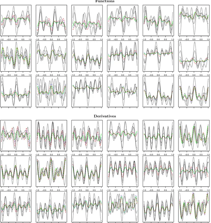
In Fig. 1 it is plotted: one dataset of curves and derivatives (black lines); the regression functions f

(

xi

)

⊤

β(

t

)

and f

(

xi

)

⊤

β

′

(

t

)

(green lines); the SBLUE predictions f

(

xi

)

⊤



β

(R)

(

t

)

and f

(

xi

)

⊤



β

(R)_′

(

t

)

(blue lines); the OLS predictions

f

(

xi

)

⊤



β

₁_/₂

(

t

)

and f

(

x_i

)

⊤



β

₁_/₂′

(

t

)

(red lines).

5.1. Dependence between functions and derivatives

We consider three different scenarios; we generate functional data y(_ijf)

(

t

)

and y(_ijd)

(

t

)

such that 1.

(α

_i(f)

(

t

), ε

_ij(f)

(

t

))

is independent on

(α

_i(d)

(

t

), ε

(_ijd)

(

t

))

;

2.

(α

_i(f)

(

t

), ε

_ij(f)

(

t

))

and

(α

(_id)

(

t

), ε

_ij(d)

(

t

))

are mildly dependent (the degree of dependence is randomly obtained);

3.

(α

_i(f)

(

t

), ε

_ij(f)

(

t

))

and

(α

_i(d)

(

t

), ε

(_ijd)

(

t

))

are fully dependent:

(α

_i(d)

(

t

), ε

(_ijd)

(

t

)) = (α

_i(f)′

(

t

), ε

(_ijf)′

(

t

))

, and hence y(_ijd)

(

t

) =

y(_ijf)′

(

t

)

.

The performance of the different estimators is evaluated by comparing the H1-norm of the p-components of the

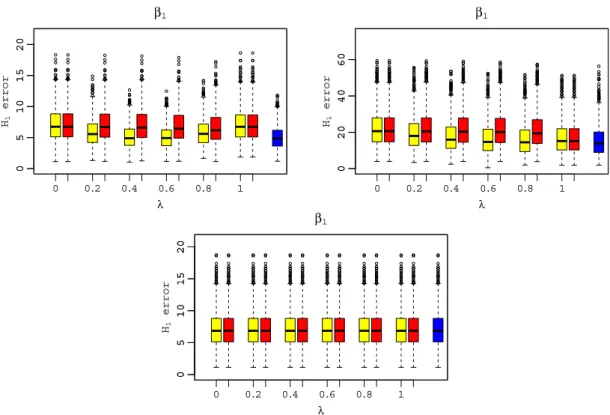
estimation errors.Fig. 2depicts the Monte Carlo distribution of the H1-norm of the first component:

∥ ˆ

βλ,

₁

(

t

) − β

₁

(

t

)∥

_H1for

different values of

λ

(red box-plot,(6)),

∥ ˆ

β

(_λ,c)₁

(

t

)−β

₁

(

t

)∥

_H1for different values of

λ

(yellow box-plots) and

∥

β

(R)

1

(

t

)−β

1

(

t

)∥

H1

(blue box-plot).

From the comparison of the box-plots corresponding to

λ =

0 and

λ =

1 with the other cases, we observe that it is always more convenient to use the whole information on y(f)

₍

_t

₎

_{and y}(d)

₍

_t

₎

_{(this behaviour is more evident in scenario 1).}

Among the three estimators

β

ˆ

(_λc)

(

t

)

,

β

ˆ

_λ

(

t

)

and



β

(R)

(

t

)

, the SBLUE is the most precise, as expected. When there is a one-to-one dependence between y(f)

(

t

)

and y(d)

(

t

)

, one source of information is redundant and all the functional estimators coincide (bottom panel ofFig. 2).

5.2. Spread of functions and derivatives

Also in this case, we consider three different scenarios. Let

rll

=



Σ_βˆ(f)



ll



Σ_βˆ(d)



ll

,

l

=

1

, . . . ,

p

,

(9)

Fig. 1. Simulated data from model(2)and predicted curves. Black lines: simulated data of curves (top panel) and derivatives (bottom panel). In each ith box (i=1, . . . ,18) the j=1, . . . ,3 replications are plotted. Blue lines: predictions based on SBLUE estimator. Red lines: predictions based on OLS estimator. Green lines: theoretical curves f(xi)⊤β(t)in top panel and f(xi)⊤β

′

(t)in bottom panel. (For interpretation of the references to colour in this figure legend, the reader is referred to the web version of this article.)

whereΣ·denotes the H1-global covariance matrix defined in(4). We generate functional data y(_ijf)

(

t

)

and y(_ijd)

(

t

)

with a different spread, such that

1. rll

∼

=

0

.

25 (in this sense, y( f)

ij

(

t

)

is ‘‘more concentrate’’ than y

(d)

ij

(

t

)

);

2. rll

∼

=

1 (y(ijf)

(

t

)

and y

(d)

ij

(

t

)

have more or less the same spread);

3. rll

∼

=

4 (y(ijd)

(

t

)

is ‘‘more concentrate’’ than y

(f) ij

(

t

)

).

As before, the performance of the different estimators is evaluated by comparing the H1-norm of the p-components of the estimation errors.Fig. 3depicts the Monte Carlo distribution of the H1-norm of the first component:

∥ ˆ

βλ,

₁

(

t

) − β

₁

(

t

)∥

_H1for

(10)

Fig. 2. H1_{norm of the first components estimation errors, for compound OLS estimators (yellow box-plots), OLS estimators (red box-plots), SBLUE} estimators (blue box-plots). Top-left panel: scenario 1, independence. Top-right panel: scenario 2, mild dependence. Bottom panel: scenario 3, full dependence. (For interpretation of the references to colour in this figure legend, the reader is referred to the web version of this article.)

Fig. 3. H1_{norm of the first components estimation errors, for compound OLS estimators (yellow box-plots), OLS estimators (red box-plots), SBLUE} estimators (blue box-plots). Top-left panel: scenario 1, independence. Top-right panel: scenario 2, mild dependence. Bottom panel: scenario 3, full dependence. (For interpretation of the references to colour in this figure legend, the reader is referred to the web version of this article.)

(11)

different values of

λ

(red box-plot,(6)),

∥ ˆ

β

(_λ,c)₁

(

t

)−β

₁

(

t

)∥

_H1for different values of

λ

(yellow box-plots) and

∥

β

(

R)

1

(

t

)−β

1

(

t

)∥

H1

(blue box-plot).

From the comparison of the box-plots of

β

ˆ

(_λc)

(

t

)

and

βλ

ˆ

(

t

)

corresponding to

λ =

0 and

λ =

1 with the other cases, it seems more convenient to use just the ‘‘less spread’’ information: y(f)

₍

_t

₎

_{in Scenario 1 and y}(d)

₍

_t

₎

_{in Scenario 2. Comparing}

the precision of

β

ˆ

(_λc)

(

t

)

and

βλ(

ˆ

t

)

with the one of the



β

(R)

(

t

)

, however, the SBLUE is the most precise, as expected. Hence, we suggest the use of the whole available information through the use of the SBLUE. Of course, when one of the sources of information has a spread near to zero then the most precise estimator is the one that uses just that piece of information and



β

(R)

(

t

)

reflects this behaviour.

6. Summary

Functional data are suitably modelled in separable Hilbert spaces (see Horváth and Kokoszka [7] and Bosq [4]) and L2is usually sufficient to handle the majority of the techniques proposed in the literature of functional data analysis.

Instead we consider proper Sobolev spaces; since we guess that the data may provide information on both curve functions and their derivatives. The classical theory for linear regression models is extended in this context by means of the sample of Riesz representatives. Roughly speaking, the Riesz representatives are ‘‘quantities’’ which incorporate both functions and their associated derivative information in a non trivial way. A generalization of the Riesz representatives are proposed to take into account the possible correlation between curves and derivatives. These generalized Riesz representatives are called just ‘‘representatives’’.

Using a sample of representatives, we prove a strong, generalized version of the well known Gauss–Markov theorem for functional linear regression models. Despite the complexity of the problem, we obtain an elegant and simple solution through the use of the representatives which belong to a Sobolev space. This result states that the proposed estimator, which takes into account both information about curves and derivatives (throughout the representatives), is much more efficient than the usual OLS estimator based only on one sample of functions (curves or derivatives). The superiority of the proposed estimator is also showed in the simulation study described in Section5.

Appendix. Proofs

Proof of Theorem 1. Part (a). We consider the sum of square residuals:

S

β(

t

)



=

r



j=1 n



i=1



∥

y(_ijf)

(

t

) −

f

(

xi

)

⊤

β(

t

)∥

2_L2

+ ∥

y( d) ij

(

t

) −

f

(

xi

)

⊤

β

′

(

t

)∥

2_L2



=

r



j=1 n



i=1



⟨

y(_ijf)

(

t

) −

f

(

xi

)

⊤

β(

t

),

y(ijf)

(

t

) −

f

(

xi

)

⊤

β(

t

)⟩

L2

+ ⟨

y_ij(d)

(

t

) −

f

(

xi

)

⊤

β

′

(

t

),

yij(d)

(

t

) −

f

(

xi

)

⊤

β

′

(

t

)⟩

L2

.

The Gâteaux derivative of S

(·)

at

β(

t

)

in the direction of g

(

t

) ∈ (

H1

₎

p_is

lim h→0 S

(β(

t

) +

hg

(

t

)) −

S

(β(

t

))

h

=

2



r



j=1 n



i=1



⟨

y(_ijf)

(

t

) −

f

(

x_i

)

⊤

_β(

t

),

f

(

x_i

)

⊤_g

₍

t

)⟩

_L2

+ ⟨

y(_ijd)

(

t

) −

f

(

x_i

)

⊤

β

′

(

t

),

f

(

x_i

)

⊤g′

(

t

)⟩

_L2





=

2r



⟨

F⊤y

¯

(f)

₍

_t

_{) −}

_F⊤ F

β(

t

),

g

(

t

)⟩(

_L2₎p

+ ⟨

F⊤y

¯

(d)

(

t

) −

F⊤F

β

′

(

t

),

g′

(

t

)⟩(

_L2₎p

,

(A.1) wherey

¯

(f)

₍

_t

₎

_and_y

_¯

(d)

₍

_t

₎

_{are two n}

_×

_{1 vectors whose ith elements are}

¯

y(_if)

(

t

) =

r



j=1 y(_ijf)

(

t

)

r

,

y

¯

(d) i

(

t

) =

r



j=1 y(_ijd)

(

t

)

r

.

(A.2)

Developing the right-hand side of(A.1), we have that the Gâteaux derivative is

=

2r





⟨

F⊤y

¯

(f)

(

t

),

g

(

t

)⟩

₍_L2₎p

+ ⟨

F⊤y

¯

(d)

(

t

),

g′

(

t

)⟩

₍_L2₎p



−



⟨

F⊤F

β(

t

),

g

(

t

)⟩

₍_L2₎p

+ ⟨

F⊤F

β

′

(

t

),

g′

(

t

)⟩

₍_L2₎p





=

2r



⟨

F⊤y

¯

(

t

),

g

(

t

)⟩(

_H1₎p

− ⟨

F⊤F

β(

t

),

g

(

t

)⟩(

_H1₎p

,

(A.3)

wherey

¯

(

t

)

is a n

×

1 vector whose ith element is the Riesz representative of



¯

y(_if)

(

t

), ¯

y(_id)

(

t

)



.