Chapter 4 Waveform analysis

Chapter 4

Waveform analysis

In the previous paragraphs we have analysed the concept of passive radar exploiting digital waveforms. In this part we decide to analyze the DVB-T signal and the UMTS signal. In order to understand the suitability of these waveforms for radar purposes, a careful study of the expected performances in terms of range resolution, Doppler resolution, Side Lobe Levels (SLL) has been carried out.

As first step we generated these waveforms through simulators compliant to the corresponding communication standards. In the next paragraphs we present the DVB-T and UMST signal key features, the simulators and after that a study of ambiguity functions of both waveforms.

4.1

Opportunity Signals study

4.1.1.DVB-T SIGNAL Simulation

DVB-T is an abbreviation for Digital Video Broadcasting — Terrestrial; it is the DVB European-based consortium standard for the broadcast transmission of digital terrestrial television. This system transmits compressed digital audio, video and other data in an MPEG transport stream, using coded orthogonal frequency-division multiplexing (COFDM) modulation. Rather than carrying the data on a single radio frequency (RF)

carrier, COFDM works by splitting the digital data stream into a large number of slower digital streams, each of which digitally modulate a set of closely spaced adjacent carrier frequencies. COFDM copes very well with multipath propagation conditions and offers a high degree of frequency economy by allowing the use of Single Frequency Networks. In the case of DVB-T, there are two choices for the number of carriers known as 2K-mode or 8K-mode. These are actually 1,705 or 6,817 carriers that are approximately 4 kHz or 1 kHz apart. DVB-T offers three different modulation schemes (QPSK, 16QAM, 64QAM) [26].

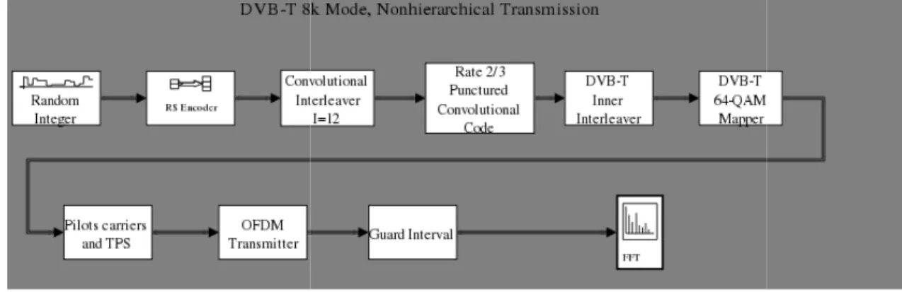
Figure 4.1 shows a simplified block diagram of DVB-T transmission system. The processing applied to MPEG-2 streams consists of channel coding (red Solomon, convolutional codes etc) and orthogonal frequency division multiplexing (OFDM). The combination of these processes form the COFDM (Code OFDM). In OFDM, a large number of closely-spaced orthogonal sub carriers are used to carry data.

Figure 4.1 DVB-T transmission system

OFDM transmission technique is robust against multipath propagation, therefore the usage of OFDM should imply more robustness of the radar system with respect to multipath propagation. The transmitted signal is organized in frames. Each frame has a duration of TF, and consists of 68 OFDM symbols.Four frames constitute one

super-frame. Each symbol is constituted by a set of K = 6 817 carriers in the 8K mode and K = 1 705 carriers in the 2K mode and transmitted with a duration TS. It is composed of two

parts: a useful part with duration TU, and a guard interval part with duration TG. The

guard interval consists in a cyclic continuation of the useful part, TU, and is inserted

before it. The symbols in an OFDM frame are numbered from 0 to 67. All symbols contain data and reference information. Since the OFDM signal comprises many separately-modulated carriers, each symbol can in turn be considered to be divided into

cells, each corresponding to the modulation carried on one carrier during one symbol [26]. In addition to the data the OFDM frame contains:

• Scattered pilot carriers • Continual pilot carriers

• Transmission Parameter Signalling (TPS) carriers

The pilots are used for frame synchronization, frequency synchronization, time synchronization, channel estimation etc.

The carriers are K=1704 in 2K mode and K=6816 in 8k mode. The spacing between carriers is 1/TU. Then the effective bandwidth of DVB-T signal is 6.71 MHz as we can

see in Table 4.1.

Parameter 8K mode 2K mode

Number of carriers 6817 1705

Duration TU 896 µs 224 µs

Carrier Spacing 1/TU 1116 Hz 4464 Hz

Effective bandwidth 6817/TU=7.61 MHz 1704/TU=7.61 MHZ

Table 4.1 OFDM parameters for DVB-T signal

The transmitted baseband signal model is defined in the following equation:

(

)

s( t )

c

p t

mT e

=

∑ ∑

−

(4.1)

• m is OFDMS symbol number

• k is the carrier number into the OFDM symbol

• ( m )

k

c is the generic constellation symbol relative to the m-th OFDM symbol and the k-th subcarrier,

•

p(t )

T

The ( m ) k

c values are normalized according to the modulation alphabet used for the data (QPSK, 16-64 QAM). The normalization factors yield

E c



_



_

=

1





The Scattered and Continual pilot carriers are transmitted at boosted power so that for these

E c



_



_

=

16 / 9





{ }

(

)

{ }

4 3 x 2 1 2

0

c

/

/

w

c

ℜ

=

−

ℑ

=

(4.2)

where wk is a series of values derived from a Pseudo-Random Binary Sequence

(PRBS), that is different for each transmitted channel [26]. Each continual pilot coincides with a scattered pilot every fourth symbol; the number of useful data carriers is constant from symbol to symbol: 1 512 useful carriers in 2K mode and 6 048 useful carriers in 8K mode. The location of scattered pilots inside the OFDM symbol depends on a specific algorithm to establish the scattered locations with a periodicity of 4 OFDM symbol. On the contrary the continual pilots have fixed locations.

TPS (Transmission Parameter Signalling) pilots, are transmitted on fixed locations, conveying information on: modulation mode, hierarchy mode, guard interval type, inner code rates, transmission mode, frame number in a super frame (i.e. 4 DVB-T frames) [26]. TPS carriers are DBPSK modulated, similar to Continual and scattered pilots, and are transmitted at normal power level. Also TPS carriers are modulated according the pseudo random sequence used for continual and pseudorandom pilots.

Figure 4.2 Frame structure

As we can see in eq.(4.1), to calculate the COFDM symbols the inverse fast Fourier transform (IFFT) algorithm is used.The start of every COFDM symbol is preceded by a guard interval. The purpose is to enhance immunity to echoes and reflections. As long as the echoes fall within the guard interval they will not affect the receivers ability to safely decode the useful data. The longer the guard interval is the higher will be the echo delays that can be tolerated. The guard interval length TG may have four different

values: TU/4, TU/8, TU/16, or TU/32.Moreover it is added by taking copies of the last of

NTG/TU samples and appending them in front to the COFDM symbol.

Figure

Figure 4.4 shows the DVB-T signal simulator complaint to the ETSI standard. The simulator manages all the key features regarding the OFDM modulation. Moreover the channel coding, including red Solomon, convolutional codes and punctured convolutional code ( inside the inner

spectrum of a DVB-T signal generated with DVB

Figure

Figure 4.3 Time-frequency OFDM structure

T signal simulator complaint to the ETSI standard. The simulator manages all the key features regarding the OFDM modulation. Moreover the channel coding, including red Solomon, convolutional codes and punctured convolutional code ( inside the inner interleave block), has been implemented. The

T signal generated with DVB-T simulator is shown in

Figure 4.4 DVB-T simulator 8k

T signal simulator complaint to the ETSI standard. The simulator manages all the key features regarding the OFDM modulation. Moreover the channel coding, including red Solomon, convolutional codes and punctured block), has been implemented. The

Figure 4

4.1.2.UMTS simulation

In this section, we provide an overview of the UMTS signal for downlink communication.

The principal features that induced us to study the UMTS sig

•••• The signal bandwidth is relatively high (5 MHz) especially if compared with GSM which offers only a 160 kHz channel. This implies in theory an improved range resolution.

4.5 DVB-T signal spectrum generated with Simulator

UMTS simulation

In this section, we provide an overview of the UMTS signal for downlink

The principal features that induced us to study the UMTS signal are:

The signal bandwidth is relatively high (5 MHz) especially if compared with GSM which offers only a 160 kHz channel. This implies in theory an improved range resolution.

T signal spectrum generated with Simulator

In this section, we provide an overview of the UMTS signal for downlink

nal are:

The signal bandwidth is relatively high (5 MHz) especially if compared with GSM which offers only a 160 kHz channel. This implies in theory an improved

•••• The UMTS FDD (Frequency Division Duplexing) frequencies spans from 2110-2170 MHz. It is therefore easier to work with directive antennas unlike the VHF band passive radars.

•••• The codes (especially the scrambling ones) guarantee very low cross-correlation levels.

•••• The growing coverage of UMTS signals on the national and international territory makes a multistatic radar configuration feasible.

Two different methods are defined for base station subscriber communication:

• FDD (Frequency Division Duplex), where uplink and downlink channels use different carriers. The carrier frequencies span from 2110-2170 MHz for downlink and 1920-1980 for uplink.

• TDD (Time Division Duplex), where uplink and downlink share the same carrier in different time slots. The carrier frequencies span from 1900 -1920 MHz and 2010-2025 MHz.

The here presented study is focused on the UMTS-FDD downlink physical channels that are defined by a specific carrier frequency, scrambling code, and channelization codes. The downlink functional block diagram is summarized as in Figure 4.6.

Figure 4.6 Downlink phisical channel

by a OVSF (Orthogonal Variable Spreading Factor) codes that preserve the orthogonality between different physical channels. This is represented by Cch,SF,m where

ch stands for channelization, SF is the spreading factor of the code and m is the code number, 0 < m <= SF-1. Afterwards the spread channel is scrambled by sequences of Gold codes. The scrambling codes (Sdl,n) are divided into 512 sets; each set consists of a

primary scrambling code and 15 secondary scrambling codes. Each UMTS cell is provided with a unique primary scrambling code that is used for base station discrimination. The scrambling codes are repeated every 10 ms radio frame. All the physical channels are scrambled except the SCH (Synchronisation CHannel ) that used by the customers for searching the cell and capturing the scrambling code. All downlink physical channels are combined using complex addition. The modulating chip rate is 3.84 Mcps (Mega chips per second). The transmit pulse-shaping filter is a root-raised cosine (RRC) with roll-off α=0.22. The physical channels are carried on a frame structure. The radio frame duration is 10 ms or 38400 chips, each frame is subdivided in 15 slots. Each time slot consists of 2560 chips.

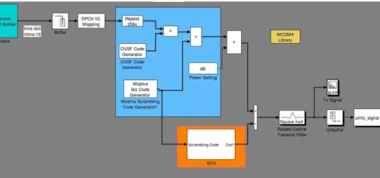
In order to obtain some performance evaluations, we have created a Simulink® model based on the WCDMA library for simulating the baseband UMTS signal. The implemented architecture is compliant with the Third Generation Partnership (3GPP) technical specifications (Figure 4.7).

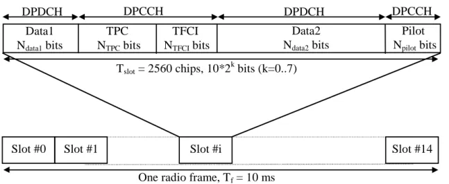
More precisely the simulated signal is relative to a downlink communication data channel with a single user and the Synchronization Channel (SCH) (highlighted in orange in Figure 4.7) in FDD mode. The Dedicated Transport Channel (DCH), containing the data stream, is transmitted in time division multiplex with control information generated at Level 1. The downlink Dedicated Physical Channel (DPCH) can be seen as a time division multiplexing of a Dedicated Physical Data Channel (DPDCH) and a Dedicated Physical Control Channel (DPCCH), as shown in Figure 4.8 where the downlink DPCH frame format is presented.

Figure 4.8 Frame structure for downlink DPCH

The k parameter determines the number of bits per slot, it is related to the spreading factor of the physical channel SF=512/2k. The number of bit for each of the fields is summarised in Table I where the slot format is reported.

This operation is simulated by the “Source: Slot builder” of Figure 4.7. A detailed view of the mentioned block is shown in Figure 4.9.

One radio frame, Tf = 10 ms

TPC NTPC bits

Slot #0 Slot #1 Slot #i Slot #14

Tslot = 2560 chips, 10*2 k bits (k=0..7) Data2 Ndata2 bits DPDCH TFCI NTFCI bits Pilot Npilot bits Data1 Ndata1 bits DPDCH DPCCH DPCCH

Figure 4.9Detailed view of Source:Slot builder Slot Format #i Channel Bit Rate (kbps) Channel Symbol Rate (ksps) SF Bits/ Slot DPDCH Bits/Slot DPCCH Transmitted slots per radio frame Bits/Slot NTr

NData1 NData2 NTPC NTFCI NPilot

0 15 7.05 512 10 0 4 2 0 4 15 1 15 7.05 512 10 0 2 2 2 4 15 2 30 15 256 20 2 14 2 0 2 15 3 30 15 256 20 2 12 2 2 2 15 4 30 15 256 20 2 12 2 0 4 15 5 30 15 256 20 2 10 2 2 4 15 6 30 15 256 20 2 8 2 0 8 15 7 30 15 256 20 2 6 2 2 8 15 8 60 30 128 40 6 28 2 0 4 15 9 60 30 128 40 6 26 2 2 4 15 10 60 30 128 40 6 24 2 0 8 15 11 60 30 128 40 6 22 2 2 8 15 12 120 60 64 80 12 48 4 8* 8 15 13 240 120 32 160 28 112 4 8* 8 15 14 480 240 16 320 56 232 8 8* 16 15 15 960 480 8 640 120 488 8 8* 16 15 16 1920 960 4 1280 248 1000 8 8* 16 15

In order to produce the data streams NData1 and NData2 we have used random sources. The slot format is customizable by the end-user even though it is usually the network

itself that manages it in function of the requested type of service. The following block inserts the Orthogonal Variable Spreading Factor (OVSF) code and subsequently the scrambling is performed. Finally the modulation is applied through the Raised Cosine Filter (RRC) and moreover the signal power can be set.

As we already said, the SCH channel is the only channel that is not scrambled and is used by the user to search for active and neighbouring cells. This channel consists of two sub-channels, the P-SCH ( Primary SCH) and S-SCH ( Secondary SCH ).

The 10 ms radio frames of the Primary and Secondary SCH are divided into 15 slots, each of length 2560 chips. Figure 4.10 illustrates the structure of the SCH radio frame. The Primary SCH consists of a modulated Galois code of length 256 chips, the Primary Synchronisation Code (PSC) denoted cp in Figure 4.10, transmitted once every slot. The

PSC is the same for every cell in the system. The Secondary SCH is also a modulated Galois code of length 256 chips, named the Secondary Synchronization Codes (SSC), but differs from the P-SCH in that it differs at every slot and repeats every frame. The Secondary Synchronization Codes (SSC) is transmitted in parallel with the Primary SCH.

Figure 4.10 Structure of Synchronisation Channel (SCH)

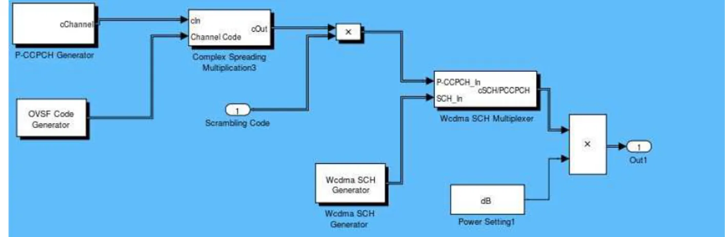
Figure 4.11 shows a detailed version of SCH block showed in Figure 4.7. Together with the SCH channel it has been simulated also the Primary Common Control Channel (P-CCPCH) that is used to carry broadcast information about the cell.

Primary SCH Secondary SCH 256 chips 2560 chips

One 10 ms SCH radio frame acsi,0 acp acsi,1 acp acsi,14 acp

Figure 4.11 SCH and P-CCPCH channels generation

The Primary CCPCH is a fixed rate (30 kbps, SF=256) downlink physical channel. This channel is not transmitted during the first 256 chips of every slots. Instead the primary and secondary channels are transmitted during this time. This allows the P-SCH and S-SCH to be transmitted with minimal interference.

Figure 4.12 Frame structure for Primary Common Control Physical Channel

The spectrum of a UMTS signal is shown in Figure 4.13. D ata

Ndata1= 18 bits

Slot #0 Slot #1 Slot #i Slot #14

Tslo t = 2560 ch ips , 20 bits

1 radio fram e: Tf = 10 m s (T x O FF)

Figure 4.13 UMTS signal spectrum generated with UMST simulink simulator

4.2

Ambiguity function analysis

As previously shown, the resolution and ambiguity in both range and Doppler are parameters of fundamental importance in the design and performance achievement of any radar system. In passive coherent location (PCL) systems, these properties are determined by the transmitted waveform, the location of the transmitter, the location of the receiver and the location of the target. In the next sections, we show an ambiguity function study for both the simulated signals.

In (4.3) we recall the ambiguity function equation:

(

)

∑

where:

• τ is the delay bin

• fD is the Doppler frequency bin

• TS is the sampling time

• N is the number of samples in the integration time

The ambiguity function has been calculated with one of the methods shown in Chapter 2.Obviously the bandwidth of both the considered waveforms is independent from the data content, and this should guarantees a constant range resolution in a monostatic configuration.

4.2.1DVB-T Ambiguity function analysis

The DVB-T signal is combination of two components:

• a random component that is obtained from MPEG-2 coding, channel coding, channel interleaving and OFDM modulation

• a deterministic component due to the guard interval and pseudo random ( or scattered) , continual and TPS carrier pilots

If we consider only the random component, we will have a thumbtack shape of ambiguity function that is an highly desirable radar waveform ( Figure 4.14).

Unfortunately, the deterministic components give rise to some ambiguities in range (delay) and Doppler domain ( Figure 4.15). As a matter of fact, the guard interval, that is a copy of the last part of the COFDM symbol, produces deterministic peaks with a period of TU (i.e. the useful symbol duration in 8k mode TU=896µs ). Furthermore,

also the pilot carriers show periodic behaviour. The continual pilot carriers are all at the same places from symbol to symbol and the pseudorandom (or scattered) pilots are repeated each 4 symbols and in addition, within the OFDM symbol they have a distance of 12/TU. Likewise also the TPS carriers are repeated from symbol to symbol.

A DVB-T signal in 8k mode has been simulated and the results about the ambiguity function are presented in Figure 4.15-Figure 4.16-Figure 4.18. The parameters of simulation are shown in Table 4.2.

Parameter Value

Useful symbol time TU 896µs

Guard interval TG TU/4=224 µs

Integration Time Tint 100 ms

Table 4.2 Simulation parameters

In Figure 4.16 the AF for zero Doppler (the Auto-ambiguity Function, ACF) is presented:

1. The red arrows show the guard interval peaks (a peak in τ=Tu very close to

another peak located in τ=TS).

2. The green arrows show the intra-symbol peaks, it should be noted peaks in TU/3,

due to continual pilots

3. The violet arrows show the inter symbol peaks mainly due to scattered and continual pilots. Moreover, because the scattered pilots are repeated every fourth symbol we expect range ambiguities occur near a delay of 4TU or a distance

more than 1500km, that outside of the range of interest for passive radar systems.

Figure 4.16 Range profile ( freq Doppler null) : green arrows intra interval peaks, violet arrows inter

Figure 4.17

From Figure 4.17 it possible to extract a time resolution around 0.131

terms of monostatic range resolution. Moreover the value of Side Lobe Level is around 27 dB.

nge profile ( freq Doppler null) : green arrows intra-symbol peaks, red arrows guard interval peaks, violet arrows inter-symbol peaks

17 Detailed view of the range profile showed in Figure

it possible to extract a time resolution around 0.131

terms of monostatic range resolution. Moreover the value of Side Lobe Level is around

symbol peaks, red arrows guard

Figure 4.16

it possible to extract a time resolution around 0.131 µs or 20 m in terms of monostatic range resolution. Moreover the value of Side Lobe Level is around

Figure 4.18

In Figure 4.18 the Doppler profile of the auto possible to distinguish the typica

of Doppler profile around the main lobe, and the Doppler resolution is around 10 Hz that is equal to the inverse of integration time. In addition, it is possib

Side Lobe Level (SLL) of 13 dB.

Figure 4.19Detailed view of Doppler profile from 18 Doppler profile DVB-T signal 8k mode

the Doppler profile of the auto-ambiguity function is presented, it is possible to distinguish the typical sinc shape. In fact, Figure 4.19 shows a detailed view of Doppler profile around the main lobe, and the Doppler resolution is around 10 Hz that is equal to the inverse of integration time. In addition, it is possible to evaluate a Side Lobe Level (SLL) of 13 dB.

Detailed view of Doppler profile from Figure 4.18

ambiguity function is presented, it is shows a detailed view of Doppler profile around the main lobe, and the Doppler resolution is around 10 Hz le to evaluate a

4.2.2UMTS Ambiguity function analysis

The UMTS signal is obtained from orthogonal codes and this should guarantee low cross correlation level. As we know, the ambiguities are mainly due to periodic components. The UMTS signal has two components that give rise to ambiguities peaks: the SCH channel and the Scrambling code. As previously mentioned, the SCH consists of a code of length 256 chips transmitted once every slot ( i.e. once every 2560 chips or 666 µs) and the scrambling code is applied to all UMTS channels and is repeated each time frame or 10 ms.

The integration time Tint used for the next graphs is Tint=50 ms.

In Figure 4.20 a Range profile is shown and the peaks due to the synchronization channel are clearly visible. These range ambiguities occur each 666 µs or each 100 km that is completely outside of the range of interest for a UMTS passive radar.

Figure 4.20 Range Profile UMST signal

The Figure 4.21 shows the UMTS ambiguity function for fd from -1kHz to 1kHz and τ

from −2µs to 2µs. It should be noted that there are sidelobes along the range on the ambiguity surface each 100 Hz due to the periodicity of scrambling code (10 ms).

- 2 - 2- 2 - 2 - 1 . 5- 1 . 5- 1 . 5- 1 . 5 - 1- 1- 1- 1 - 0 . 5- 0 . 5- 0 . 5- 0 . 5 0000 0 . 50 . 50 . 50 . 5 1111 1 . 51 . 51 . 51 . 5 2222 x 1 0 x 1 0 x 1 0 x 1 0- 3- 3- 3- 3 - 1 0 0 - 1 0 0- 1 0 0 - 1 0 0 - 9 0 - 9 0 - 9 0 - 9 0 - 8 0 - 8 0 - 8 0 - 8 0 - 7 0 - 7 0 - 7 0 - 7 0 - 6 0 - 6 0 - 6 0 - 6 0 - 5 0 - 5 0 - 5 0 - 5 0 - 4 0 - 4 0 - 4 0 - 4 0 - 3 0 - 3 0 - 3 0 - 3 0 - 2 0 - 2 0 - 2 0 - 2 0 - 1 0 - 1 0 - 1 0 - 1 0 0 0 0 0 s e c s e cs e c s e c d B d B d B d B

Figure 4

Figure 4.22shows the range profile (f range ambiguity is 0.39µs.

Figure 4.22 SLL -20 @ -0.69 µs

fd,Hz

4.21 Ambiguity funtion for UMTS signal

shows the range profile (fd = 0), where the sidelobe levels are

Range Profile of ambiguity function ( fd=0 )

SLL -14.6 @ 0.39 µs

τ,µs

Figure 4.23shows the Doppler profile (τ = 0), where the sidelobe levels are -13.5dB and the Doppler ambiguity is 28.6 Hz. As almost all digital waveforms the zero levels are in multiple of 1/Tint .

Figure 4.23 Doppler Profile of ambiguity function

The simulations have proven that the theoretical range resolution is around 33 m or 0:22 µs. While the Doppler resolution depends on the integration time and in this case with Tint = 0; 05s is equal to 20 Hz.

Figure 4.24 shows the ambiguity function relative to different scrambling codes which is what happens when the signals come from different basestations. Thanks to the properties of scrambling codes the correlation levels are very low, the mean level is -50 dB.

-1000 -800

-600

-400

-200

0

200

400

600

800

-50

-40

-30

-20

-10

Hz

|

ψ

(0

,

ν

)|

d

B

UMTS Ambiguity Function: Simulated Data (

τ

=0)

Figure 4.24 Cross-Ambiguity function between signals coming from different basestations

4.3

Preliminary measurements

4.3.1RF Front End Choice

In order to do a preliminary measurements we needed to identify a daughterboard able to acquire both of DVB-T and UMTS signals.

The DBSRX daughterboard allows to capture signal from 800 MHz and 2400 MHz ( Figure 4.25 ).

Figure 4.25 DBSRX daughterboard

Figure

The schematics reveals three main blocks within the DBSRX:

• MGA8256 amplifier that captures the RF signal from antenna • MAXIM MAX2118 is a low cost direct conversion tuner, that

the base band the RF signal

• 2 AD8132 amplifiers take the signal from MAX2118 and send it to the ADCs USRP converters with right levels of power

igure 4.26 DBSRX block diagram

three main blocks within the DBSRX:

MGA8256 amplifier that captures the RF signal from antenna MAXIM MAX2118 is a low cost direct conversion tuner, that down the base band the RF signal

2 AD8132 amplifiers take the signal from MAX2118 and send it to the ADCs USRP converters with right levels of power

down-converts to

.

The main features of DBSRX are made by the MAX2118 (Figure 4.27) This device provides:

• a programmable broadband I/Q down-converter. • programmable gain controls:

o one gain control is at RF stage ( 0-56 dB) GC1 in Figure 4.27

o 2 gain control are at baseband stage ( 0-24 dB), GC2 in Figure 4.27

• a baseband low-pass filter cut-off frequency control. The adjustable bandwidth is from 2 MHz to 33 MHz

The RF and baseband variable gain amplifiers provide more than 79dB of gain control range. Tuning the down-converter on the DBSRX, consists of programming the value of two dividers (Figure 4.27). The R divider divides down the reference clock frequency. The N divider divides down the LO frequency. The R divider has a range from 2 to 256, the N divider from 256 to 32768. The value of DBSRX frequency is:

refclk DBSRX f f N R =

(4.4)

The PLL in the Max2118 is unstable if it is required to divide down the reference clock frequency to below 250 kHz, this effectively limits the frequency resolution at which it is possible to command the LO frequency. However the right value of frequency can be set if we record the residual frequency and we send it to the DDCs on the USRP.

As a preliminary step, DVB-T and UMTS signal have been acquired through the USRP board equipped by DBSRX daughterboard . At this stage the acquisition has been done with one USRP complex receiving channel working at 8 MSps.

The antennae used were an ominidirectional patch antenna working around 2 GHz for UMST signal and a dipole antenna for DVB

presented in Figure 4.28

Figure 4

The data has been acquired then memorized on Personal computer and processed wit Matlab functions.

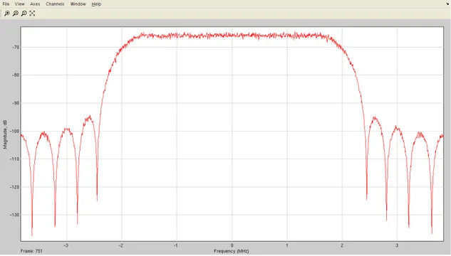
Figure 4.29 shows a DVB-T spectrum acquired in real time through the USRP board relevant to the ”La7” emitted from a repeater located on Monte Serra mountain close to Pisa. The central frequency is at 818 MHz a

bandwidth. The OFDM modulation is clearly visible in the spectrum behaviour havin flat signal bandwidth.

The antennae used were an ominidirectional patch antenna working around 2 GHz for UMST signal and a dipole antenna for DVB-T signal. The acquisition scheme is

4.28 Acquisition scheme with one channel

The data has been acquired then memorized on Personal computer and processed wit

T spectrum acquired in real time through the USRP board relevant to the ”La7” emitted from a repeater located on Monte Serra mountain close to Pisa. The central frequency is at 818 MHz and the signal exhibits about 8 MHz of bandwidth. The OFDM modulation is clearly visible in the spectrum behaviour havin The antennae used were an ominidirectional patch antenna working around 2 GHz for

he acquisition scheme is

The data has been acquired then memorized on Personal computer and processed with

T spectrum acquired in real time through the USRP board relevant to the ”La7” emitted from a repeater located on Monte Serra mountain close to nd the signal exhibits about 8 MHz of bandwidth. The OFDM modulation is clearly visible in the spectrum behaviour having a

Figure 4.29 DVB-T signal spectrum 818 MHz

Figure 4.30 shows the measured UMTS real time spectrum for a downlink signal of a basestation close to the Department of Information Engineering located in Pisa. The carrier is at 2.1675 GHz and the bandwidth is about 5 MHz, the Root Raised Cosine shape, owing to the UMTS signal, is easily identifiable.

Both DVB-T and UMTS signals have been acquired for a long time interval and samples recorded.

4.3.2Comparisons between real and simulated ambiguity functions

Ambiguity functions have been computed and compared with the ones obtained by simulation. Plots of the ambiguity function along time delay (range) and Doppler frequency and in 3D view are presented from

signal and from Figure 4.34 to

An integration time Tint=50 ms has been used.

Figure 4.31

As expected, the AF of the DVB

side peaks due to pilot carriers and the guard interval, as we reported in section

tween real and simulated ambiguity functions

Ambiguity functions have been computed and compared with the ones obtained by simulation. Plots of the ambiguity function along time delay (range) and Doppler frequency and in 3D view are presented from Figure 4.31 to Figure 4.33

to Figure 4.36 for UMTS signal. =50 ms has been used.

31 3D view of DVB-T Ambiguity Function

As expected, the AF of the DVB-T signal exhibits a desired main peak but also a set of ilot carriers and the guard interval, as we reported in section

tween real and simulated ambiguity functions

Ambiguity functions have been computed and compared with the ones obtained by simulation. Plots of the ambiguity function along time delay (range) and Doppler 33 for DVB-T

T signal exhibits a desired main peak but also a set of ilot carriers and the guard interval, as we reported in section 4.2.2.

Figure 4.32 DVB-T ambiguity function: range profile

Figure 4.33 DVB-T ambiguity function:Doppler profile

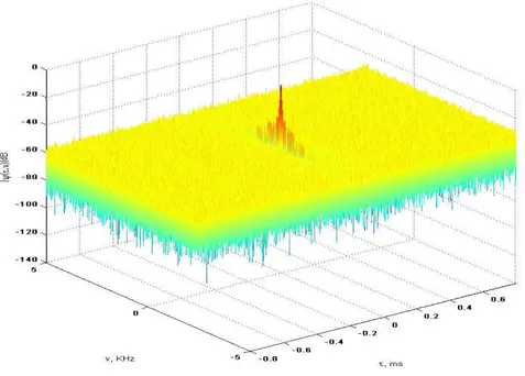
UMTS real data confirm the previous analysis done 4.2.2: the time resolution is 0.22µs (i.e.: a range resolution of 33 m in monostatic configuration) and the Doppler resolution depends on integration time (e.g.: 20 Hz for Tint=50 ms).

The 3D UMTS AF plot (Figure 4.34) reveals the presence of lines along the range repeated every 100 Hz due to the periodicity of the scrambling code sequence (i.e.: frame duration is equal to 10 ms).

Figure 4.34

Range and Doppler AF profiles are shown in

AF range profile shows only a secondary peak at 666 synchronization channel (SCH) content.

Figure 4.35

34 3D view of DVB-T Ambiguity Function

Range and Doppler AF profiles are shown in Figure 4.35 and Figure 4.36

AF range profile shows only a secondary peak at 666 µs due to the periodicity of the synchronization channel (SCH) content.

35 UMTS ambiguity function: range profile

36. The UMTS s due to the periodicity of the

Figure

All the plots have show

they validate the theoretical study. Results of this section are partially shown in

Figure 4.36 UMTS ambiguity function: Doppler profile

shown a good matching between real data and simulated data, and y validate the theoretical study. Results of this section are partially shown in

a good matching between real data and simulated data, and y validate the theoretical study. Results of this section are partially shown in [30].

4.4

Multichannel acquisition

In order to create a passive radar

two channels. A Graphical User Interface able to capture 2 receiving has been developed (Figure 4.

DBSRXs on the USRP board. This configuration highlights the concept flexibility, typical feature of a SDR system and a requirement of our system as well. A possible weakness of this configuration is represented of the USB cable. USB cable it is possible to sustain a maximum 32 MBps, and in order to cat channels ( 8 MHz of bandwidth each)

to 8 bits. Next paragraphs consider how this trick influences our radar system.

Figure 4.37

Multichannel acquisition

In order to create a passive radar demonstrator, we needed to acquire simultaneously User Interface able to capture 2 receiving complex

.37). The GUI allows to completely configure both of the DBSRXs on the USRP board. This configuration highlights the concept

flexibility, typical feature of a SDR system and a requirement of our system as well. A possible weakness of this configuration is represented of the USB cable. USB cable it is possible to sustain a maximum 32 MBps, and in order to cat

channels ( 8 MHz of bandwidth each), the sample format must be changed from 14 bit . Next paragraphs consider how this trick influences our radar system.

37 Simultaneous acquisition on two channels

simultaneously complex channels ). The GUI allows to completely configure both of the DBSRXs on the USRP board. This configuration highlights the concept of system flexibility, typical feature of a SDR system and a requirement of our system as well. A possible weakness of this configuration is represented of the USB cable. Across the USB cable it is possible to sustain a maximum 32 MBps, and in order to catch 2 DVB-T the sample format must be changed from 14 bits . Next paragraphs consider how this trick influences our radar system.

4.5

Antenna Choice

This paragraph shows the commercial antennae chosen to build our passive radar demonstrator. Before to analyze the power budget requirements and limitations of our passive radar demonstrator.

A passive radar receiver generally presents two antenna denoted as reference and surveillance antenna. The reference antenna is used to capture the direct signal from the transmitter thus providing a reference signal to be compared with target echo. The surveillance antenna is pointed to the area of interest. The primary requirements for the surveillance or target antenna are:

• High Gain that allows target detection

• Narrow beam pattern allows a roughly estimation of Direction of Arrival (DoA) • Low Side Lobe Levels in order to have in the transmitter direction low level of

direct signal

Investigating the electronic market, we tried to find antennae compliant to previous considerations. It should be noted that is quite difficult to have narrow beam for TV antennae. In fact, they are designed to have high gain on wide beams.

The maximum gains for TV antennae are around 17-18 dB, instead for UMST antenna it is possible to have gains around 20 dB. Furthermore, the minimum beam widths are around 20° for TV antennae and 10° for UMTS antenna. The UMTS antenna beams are narrower because usually, they are used for point-to-point links.

Table 4.3 shows the main characteristics of the considered antennae. An antenna with 95 elements and 2m length has been considered to point the surveillance area and an antenna with 47 antenna has been chosen to point the illuminator of opportunity. The irradiation pattern for surveillance antenna is presented in Figure 4.38.

Antenna Frequency Gain HPBW (°) H plane E plane R 95 UHF (460-860 MHz) 10/17.5 dB 42°/19° 52°/°28° R47 UHF (460 -860 MHz) 8/15 dB 46°/24° 58°/36° Table 4.3 DVB-T antennae a) b)

Figure 4.38 a) Surveillance antenna, b)Pattern Irradiation for 95 elements antenna: black line-470 MHz, yellow line-670 MHz and red line-860 MHz

Regarding the UMTS antennae, we considered parabolic antennae working in the range from 2.1 GHz to 2.3 GHz.

Parameter Value

Gain 22.5dBi

Bandwidth 2.12-2.35GHz

3dB beam Pattern 10°x10°

Dimensions 76cm x 76 cm

Table 4.4 UMTS antenna specifications

a)

b1)

b2)