4. DESIGN AND MODELLING OF R.C. CASE STUDIES

(1)

4. DESIGN AND MODELLING OF R.C. CASE STUDIES

Different reinforced concrete case studies were designed following the prescriptions imposed by actual European and Italian standards for constructions [1, 6, 7]. Different distributions of structural elements in both plan and elevation, different functional destinations (commercial, residential and office buildings), different seismicity areas (high seismicity with a design p.g.a. equal to 0.25 g and medium seismicity with a design p.g.a. of 0.15 g) and different ductility classes (high ductility class – HDC and low ductility class – LDC) were considered; steel grade B450C and concrete class C25/30 were used for the design. Table 4.1 summarizes the r.c. buildings designed as case studies. The procedure for the design of reinforced concrete buildings was organized in several different steps, presented in the following pages.

Table 4. 1: Designed reinforced concrete case studies.

Functional destination p.g.a. [g] Ductility class Steel grade

Residential building 0,25 HDC B450C

Residential building 0,25 LDC B450C

Commercial building 0,25 HDC B450C

Office building 0,25 HDC B450C

4.1 Definition of the geometrical schemes for buildings

Moment resisting frames (MRF) with span length of beams variable between 4.0 m and 7.0 m and storey height between 2.5 m and 5.0 m were adopted for the design of the selected buildings in relation to the functional destination foreseen. The stiffening contribution of stairs and lift’s rooms was directly taken into account through the introduction of opportune elements in the numerical models described in paragraph 4.2.5.

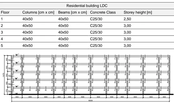
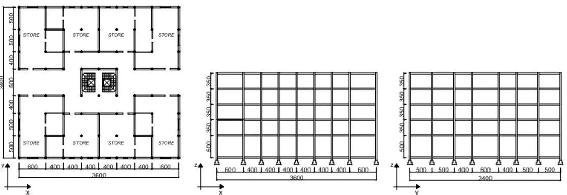
Residential buildings in both HDC and LDC present the same geometrical disposition of structural elements, resulting in an area of 60,0x14,0 m2 and a total height of 14,0 m; commercial building in HDC is characterized by an area of 36,0x34,0 m2 and a total height of 19,0 m and, finally, office building in HDC presents an area of 108,0x30,0 m2 and a global height of 19,0 m. Figures from 4.1 to 4.3 represent the geometrical schemes, in plan and elevation, of the selected case studies.

(2)

Figure 4. 1: Geometrical schemes adopted for residential buildings.

Figure 4. 2: Geometrical schemes adopted for office building.

Figure 4. 3: Geometrical schemes adopted for commercial building.

x y 400 600 600 400 400 600 600 400 400 600 600 400 6000 4 0 0 6 0 0 4 0 0 1 4 0 0 400 600 600 400 400 600 600 400 400 600 600 400 6000 3 0 0 3 0 0 3 0 0 3 0 0 1 4 5 0 2 5 0 3 0 0 3 0 0 3 0 0 3 0 0 1 4 5 0 400 600 400 1400 x z y z 2 5 0 600 700 500 500 700 700 500 500 700 700 500 500 700 700 500 500 700 600 10800 4 0 0 7 0 0 4 0 0 4 0 0 7 0 0 4 0 0 3 0 0 0 3 5 0 3 5 0 3 5 0 3 5 0 5 0 0 600 700 500 500 700 700 500 500 700 700 500 500 700 700 500 500 700 600 10800 400 700 400 400 700 400 3000 3 5 0 3 5 0 3 5 0 3 5 0 5 0 0 y z x z x y 600 400 400 400 400 400 400 600 3 5 0 3 5 0 3 5 0 3 5 0 5 0 0 x z 500 500 400 600 400 500 500 y z x y 3 5 0 3 5 0 3 5 0 3 5 0 5 0 0 600 400 400 400 400 400 400 600 3600 5 0 0 5 0 0 4 0 0 6 0 0 4 0 0 5 0 0 5 0 0 3 4 0 0 3400 STORE 3600

STORE STORE STORE

(3)

4.2 Structural design of case studies

4.2.1 Pre-sizing of structural elements for gravitational loads

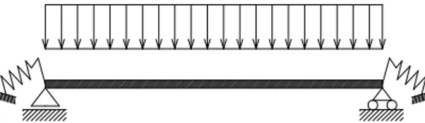
A preliminary pre-sizing of structural elements was executed considering only vertical loads, including both gravitational and live loads with reference to the selected case study; the formula provided by Eurocode [13] for the fundamental combination of loads, with opportune values of partial coefficients, was used. Simplified expressions were adopted for the definition of the bending action on beams (Eqn. 4.1) and for the individuation of the height of the section (Eqn. 4.2). A simplified static scheme, intermediate between the fully fixed and the hinged beam was considered (figure 3.4); in general, the width of the section was defined in relation to geometrical and practical considerations based on functional and architectural necessities. For sake of clarity, in the following expressions L represents the maximum length of the beam, qd is the desing load acting on the

element, b is the width of the beam’s section, d is the height of the section and r is a coefficient depending on the mechanical characteristics of materials, on the ratio between longitudinal reinforcements in tension and compression (ρ) and on the supposed modality of failure (Perrone [76]). The ratio ρ was fixed considering the limitations imposed by Eurocode 8 [1] for the seismic desing of beams: ρ shall be higher than 0.50 in correspondence of the critical zones of elements and higher than 0.25 in the other zones.

Figure 4. 4: Partially fixed scheme adopted for the pre-sizing of beams.

10

2 max ,

L

q

M

_b

=

d

⋅

(4.1)

b

M

r

d

=

⋅

b max, (4.2) The pre-sizing of column’s sections was preliminarily executed considering only the axial force, evaluated using the influence area of each structural element and the corresponding acting loads. Some indications presented in actual standards for seismic constructions were also taken into account: according to EN 1998-1:2005 [1], the normalized axial force on primary columns shall not exceed 0.65 for LDC and 0.55 for HDC (Eqn. 4.3).







≤

⋅

=

₀

0 _.

.

₆₅

55 _for

for

_LDC

HDC

c cd d

A

f

N

ν

(4.3)

(4)

4.2.2 Definition of gravitational loads

Vertical loads acting on selected case studies were defined in relation to the typology of structural and not structural elements used (for storey slab, roof, internal and external infills, equipments, etc…) and in relation to the functional destination of the buildings (for live loads).

For residential buildings in both high and low ductility class, storey slabs “Predalle H24-i50”, characterized by a total height of 24 cm and spacing between longitudinal joists equal to 50 cm were used, resulting in a vertical load (Gk) equal

to 3.35 kN/m2.

For commercial building storey slabs “Predalle H24-i40”, characterized by a total height of 24 cm and spacing between longitudinal joists equal to 40 cm were used, resulting in a vertical load (Gk) equal to 4.00 kN/m

2

. For office building storey slabs “Predalle H28-i50”, characterized by a total height of 28 cm and spacing between longitudinal joists equal to 50 cm were used, resulting in a vertical load (Gk) equal

to 3.70 kN/m2.

Moreover, additional vertical loads due to concrete slabs, floor and internal infills (considered uniformly distributed on the storey slab) were considered, resulting in values of actions respectively equal to 2.80 kN/m2, 2.35 kN/m2 and 2.50 kN/m2 for residential (both HDC and LDC), commercial and office buildings.

The values of accidental loads (Q) were derived from both Eurocodes and Italian standard for constructions [7], in relation to the functional destination chosen for each building; live loads are summarized in table 4.2. The accidental live load acting on roof slab was generally considered equal to 0.50 kN/m2 (used for not practicable roofs). Wind and snow actions were also evaluated and included in the desing according to the fundamental gravitational combination proposed by actual standards.

Table 4. 2: Loads acting on r.c. case studies. Functional Destination Ductility Class Structural loads (kN/m2)

Not structural loads (kN/m2) Q (kN/m2) Residential HDC 3,35 2,80 2,00 Residential LDC 3,35 2,80 2,00 Office HDC 3,70 2,50 3,00 Commercial HDC 4,00 2,35 5,00

4.2.3 Definition of seismic action

Seismic action was opportunely evaluated using the desing response spectra defined in Eurocode 8 [1] and taking into account also the prescriptions of actual Italian Standards for Constructions [7], in order to achieve the required level of design seismic action, expressed in terms of peak ground acceleration (p.g.a.). Buildings were designed considering soil category “B”, characterized by a speed of propagation of shear waves in the first 30 m of depth between 360 and 800 m/s. According to EN 1998-1:2005 [1] response spectrum of Type 1 can be adopted, in the assumption that earthquakes with magnitude higher than 5.5 can take place. Considering also the prescriptions imposed by D.M. 14/01/2008 [7], an opportune response spectrum was individuated for each building in relation to the effective

(5)

reference life (VR) of the structure, defined as function of the nominal life (VN) and

of the use coefficient (CU), whose values are given by the Italian standard. As an

example, for ordinary constructions, CU is assumed equal to 1.0, while for strategic

buildings (i.e. hospitals and others) and for schools is respectively equal to 2.0 and 1.5. The nominal life VN is equal to 50 years for ordinary constructions, 100 years

for strategic buildings and 10 years for temporary constructions. The desing p.g.a. (ag) and other two significative parameters (F0, related to the amplification of

spectral acceleration and TC *

, period corresponding to the beginning of the constant velocity branch of the spectrum) are opportunely defined in relation to the site in which the building is designed, considering the rigid reference soil.

For the designed case studies, the reference life VR was assumed equal to 50

years, the coefficient CU is unitary and the nominal life VN is consequently equal to

50 years; buildings were designed with reference to two different limit state, i.e. Life Safety limit state (LS), as regards strenght, and Damage Limitation limit state (DL), as regards stiffness and displacements. The return period of design seismic action (TR) can be defined through the expression 4.4, in which PVR, defined as the

probability of exceedance in the reference life, is opportunely individuated in relation to the different limit states (i.e. 63% for DL and 10% for LS).

(

VR

)

R R P V T − − = 1 ln (4.4)

For the selected buildings, the return periods of seismic action is respectively equal to 475 and 75 years for Life Safety and Damage Limitation limit states.

In order to directly take into account the global ductility of the structure, design response spectra with opportune behaviour factor “q” were adopted. The behaviour factors for case-study buildings were evaluated considering the prescriptions imposed by both actual European and Italian standards for constructions [1, 7]. The behaviour factor q is defined as the product of “reference” behaviour factor for constructions characterized by regularity in elevation (q0) and the coefficient Kr,

taking into account eventual irregularities of masses and stiffness in elevation, equal to 1.0 for regular structures and to 0.8 otherwise (Eqn. 4.5).

r

K q

q= ₀⋅ (4.5)

For reinforced concrete buildings the value of q0 is defined in table 4.3:

Table 4. 3: Values of q0 factor for regular structures in elevation (Table 5.1 EN 1998-1:2005).

Structural typology q0

LDC HDC

Moment resisting frames, coupled walls and mixed 3.0•α_u/ α₁ 4.5•α_u/ α₁

Structures with walls (not coupled) 3.0 4.0•αu/ α1

Structures with torsional deformability 2.0 3.0

Inverted pendulum structures 1.5 2.0

The values of the ratio

1 α

(6)

Table 4. 4: Values of the ratio αu/α1 for frame structures.

Frame structures with one single floor α_u/ α₁ 1.1

Frame structures with one singe span and more storeys αu/ α1 1.2

Frame structures with more spans and more storeys α_u/ α₁ 1.3

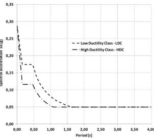
For the selected case studies, the values of the behaviour factors are summarized in the table 4.5, while figure 4.5 shows the horizontal response spectra used for design of buildings according to what prescribed by D.M. 14/01/2008 [7]. The vertical component of seismic action is not necessary for selected buildings.

Figure 4. 5: Response spectra used for the desing of case studies in high and low ductility class, for design p.g.a. equal to 0.25g (D.M.14/01/2008).

Table 4. 5: Values of the q factors adopted for designed buildings.

Functional destination p.g.a. [g] Ductility class q factor

Residential building 0,25 HDC 5,85

Residential building 0,25 LDC 3,90

Commercial building 0,25 HDC 5,85

Office building 0,25 HDC 5,85

4.2.4 Combination of actions

The fundamental combination for gravitational loads is expressed through the expression 4.6 (Eqn. 6.10 from § 6.4.3.2 of EN 1990:2006 [13]), in which Gk,j are

the gravitational loads due to structural and not structural elements, P is the pre-compression load, Qk,j are the live loads; the values of the safety partial coefficients

are defined in Table A.1.1 of Annex A1 of EN 1990:2006 [13].

i k i i i Q k Q P j k j j G G P Q 0, Q , 1 , 1 , 1 , , 1 , ⋅ + ⋅ + ⋅ +

∑

⋅ ⋅

∑

≥ ≥ ψ γ γ γ γ (4.6) 0,00 0,05 0,10 0,15 0,20 0,25 0,30 0,35 0,00 0,50 1,00 1,50 2,00 2,50 3,00 3,50 4,00 S p e ct ra l a cc e le ra ti o n S a [ g ] Period [s]

Low Ductility Class - LDC High Ductility Class - HDC

(7)

The seismic combination to be considered in the design is expressed through the expression 4.7 (Eqn. 6.12.a from § 6.4.3.2 of EN 1990:2006), in which Gk,j are the

gravitational loads due to structural and not structural elements, P is the pre-compression load, Qk,j are the live loads and AEd refers to seismic event; the values

of the safety partial coefficients are defined in Table A.1.1 of Annex A1 of EN 1990:2006 [13].

∑

≥ ≥ ⋅ + + + 1 , , 2 1 , i i k i Ed j j k P A Q G ψ (4.7)

Seismic masses to be considered in the desing are defined according to equation 3.17 of EN 1998-1:2005 [1], in which ψE,i is a coefficient used for taking into

account the possibility that accidental loads are not always totally present during a seismic event.

∑

Gk,j +

ψ

E,i ⋅Qk,i (4.8)

The values of ψE,i, according to what presented in EN 1998-1:2005 [1], are equal to

i i

E,

ϕ

ψ

2,

ψ

=

⋅

, where ψ2,i are defined in Table A.1.1 of Annex A1 of EN 1990:2006

[13] and ϕ is defined in Table 4.2 of EN 1998-1:2005 [1].

4.2.5 Linear modelling of the structures and analyses’ results

Tridimensional linear models were elaborated for each case study using SAP 2000 (v.14.1) software, according to what imposed by actual standards for seismic constructions. Mono-dimensional “frame” elements were used for both beams and columns, while for the slabs of the stairs, two-dimensional plane “shell” elements with opportune thickness were adopted. Columns were fixed at the base and opportune diaphragms were applied in correspondence of each floor in order to represent the rigid contribution of the storey slab, previously defined and characterized by a concrete slab with reinforcement grid of 40 mm of thickness. Figures from 4.6 to 4.8 present the simple schemes of the linear models, including, as already mentioned, the stiffening contribution of stairs and lift’s rooms.

As regards the choice of materials, concrete class C25/30 was adopted for concrete elements, while steel grade B450C was used for steel reinforcements. The mechanical characteristics of materials, in terms of compressive strength for concrete and yielding and tensile strenght for steel, are presented in table 4.6.

Table 4. 6: Mechanical properties of materials used in the desing.

Material Class fc [N/mm2] γc

Concrete C25/30 25 1,5

Material Steel grade Re [N/mm

2

] Rm [N/mm

2

] γs

(8)

Figure 4. 6: Tridimensional linear model for residential buildings case studies.

Figure 4. 7: Tridimensional linear model for commercial building case study.

(9)

Vertical loads were directly applied to bearing structural elements as linear distributed loads and opportune torsional moments were introduced for taking into account the effects of the centroid eccentricity, accepted to be equal to the 5% of the maximum dimension of the building in the perpendicular direction respect to the seismic action according to what prescribed by EN 1998-1:2005 [1] and D.M.14/01/2008 [7].

For taking into account the cracking phenomena of concrete at life safety limit state (LS), a reduction of stiffness of primary structural elements (beams and columns) was adopted. According to Eurocode 8 and to D.M. 14/01/2008, in r.c. structures the phenomenon of the cracking of concrete and the following loss of stiffness can be easily considered reducing the uncracked stiffness of structural elements till the 50%; for the selected case studies, according to what presented in the current literature [3, 4, 5, 77], the cracking of concrete was taken into account reducing the stiffness of structural elements in relation to the axial force and to the shape of the elements themselves, as presented in table 4.7, where Ig represents the moment of

inertia of the gross concrete sections about the centroidal axis neglecting the contribution of reinforcements and Ag is the gross concrete section area.

Table 4. 7: Recommended values for cracking of concrete elements [5].

Structural Element Range Recommended value

Rectangular beams 0,30 - 0,50 Ig 0,40 Ig T and L beams 0,25 - 0,45 Ig 0,35 Ig Columns, P > 0,5 f' c Ag 0,70 - 0,90 Ig 0,80 Ig Columns, P = 0,2 f'c Ag 0,50 - 0,70 Ig 0,60 Ig Columns, P = -0,05 f'c Ag 0,30 - 0,50 Ig 0,40 Ig

In general, a reduction of stiffness equal to 50% was adopted for beam elements and a reduction of stiffness equal to 30% was adopted for column elements, characterized by a significative axial load, for all the designed case study buildings. Linear Modal Analysis with desing response spectra was executed for the individuation of the effective actions on structural elements in both fundamental and seismic loading combination.

The seismic masses to be considered in the modal analysis were evaluated according to what prescribed by Eurocode 8, already presented in Eqn. 4.8. According to EN 1998-1:2005 [1] all the modes characterized by a participating mass higher than 5% and able to reach a total participating mass higher than 90% in each significative direction shall be considered.

The results of modal analysis on selected reinforced concrete buildings are summarized in the tables from 4.8 to 4.11, where Mx and My represent the modal

participating masses respectively in x and y direction. The values presented are evaluated considering both the uncracked and the reduced stiffness for beams and columns, according to what referred in table 4.7.

(10)

Table 4. 8: Significative results of modal analysis for residential building in HDC.

Mode Uncracked condition Cracked condition

Period MX MY Sum MX Sum MY Period MX MY Sum MX Sum MY

- Sec [%] [%] [%] [%] Sec [%] [%] [%] [%] 1 0,7836 76,3% 0,0% 76,3% 0,0% 1,0296 75,4% 0,0% 75,4% 0,0% 2 0,6098 0,0% 0,1% 76,3% 0,1% 0,7898 0,0% 0,1% 75,4% 0,1% 3 0,3890 0,0% 75,9% 76,3% 75,9% 0,5076 0,0% 75,5% 75,4% 75,6% 4 0,2420 11,9% 0,0% 88,1% 75,9% 0,3155 12,3% 0,0% 87,7% 75,6% 5 0,1981 0,0% 0,0% 88,1% 75,9% 0,2570 0,0% 0,0% 87,7% 75,6% 6 0,1277 0,0% 11,9% 88,1% 87,8% 0,1652 0,0% 11,9% 87,7% 87,5% 7 0,1219 5,7% 0,0% 93,8% 87,8% 0,1539 5,9% 0,0% 93,6% 87,5% 8 0,1041 0,0% 0,0% 93,8% 87,8% 0,1312 0,0% 0,0% 93,6% 87,5% 9 0,0731 0,0% 5,2% 93,8% 93,0% 0,0921 0,0% 5,4% 93,6% 92,9%

Table 4. 9: Significative results of modal analysis for residential building in LDC.

- Sec [%] [%] [%] [%] Sec [%] [%] [%] [%] 1 0,8055 77,7% 0,0% 77,7% 0,0% 1,0598 76,9% 0,0% 76,9% 0,0% 2 0,6334 0,0% 0,1% 77,7% 0,1% 0,8205 0,0% 0,2% 76,9% 0,2% 3 0,4282 0,0% 80,7% 77,7% 80,8% 0,5563 0,0% 79,9% 76,9% 80,1% 4 0,2475 11,6% 0,0% 89,2% 80,8% 0,3229 12,0% 0,0% 88,8% 80,1% 5 0,2038 0,0% 0,0% 89,2% 80,8% 0,2644 0,0% 0,0% 88,8% 80,1% 6 0,1384 0,0% 10,6% 89,2% 91,4% 0,1783 0,0% 10,8% 88,8% 90,9% 7 0,1252 5,4% 0,0% 94,6% 91,4% 0,1584 5,7% 0,0% 94,5% 90,9%

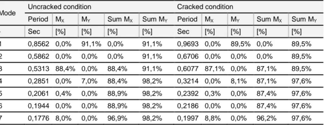
Table 4. 10: Significative results of modal analysis for commercial building in HDC.

- Sec [%] [%] [%] [%] Sec [%] [%] [%] [%] 1 0,8562 0,0% 91,1% 0,0% 91,1% 0,9693 0,0% 89,5% 0,0% 89,5% 2 0,5862 0,0% 0,0% 0,0% 91,1% 0,6706 0,0% 0,0% 0,0% 89,5% 3 0,5313 88,4% 0,0% 88,4% 91,1% 0,6077 87,1% 0,0% 87,1% 89,5% 4 0,2851 0,0% 7,0% 88,4% 98,2% 0,3214 0,0% 8,1% 87,1% 97,6% 5 0,2061 0,4% 0,0% 88,9% 98,2% 0,2392 0,3% 0,0% 87,4% 97,6% 6 0,1944 0,0% 0,0% 88,9% 98,2% 0,2186 0,0% 0,0% 87,4% 97,6% 7 0,1776 8,0% 0,0% 96,9% 98,2% 0,1997 8,8% 0,0% 96,2% 97,6%

(11)

Table 4. 11: Significative results of modal analysis for office building in HDC.

- Sec [%] [%] [%] [%] Sec [%] [%] [%] [%] 1 0,8317 0,0% 91,4% 0,0% 91,4% 0,9129 0,0% 90,4% 0,0% 90,4% 2 0,6776 86,0% 0,0% 86,0% 91,4% 0,7771 84,8% 0,0% 84,8% 90,4% 3 0,6524 0,0% 0,0% 86,0% 91,4% 0,7220 0,0% 0,0% 84,8% 90,4% 4 0,2774 0,0% 6,9% 86,0% 98,3% 0,3024 0,0% 7,4% 84,8% 97,8% 5 0,2254 0,0% 0,0% 86,0% 98,3% 0,2487 10,4% 0,0% 95,2% 97,8% 6 0,2217 10,0% 0,0% 96,0% 98,3% 0,2477 0,0% 0,0% 95,2% 97,8% 7 0,1635 0,0% 1,2% 96,0% 99,5% 0,1757 0,0% 1,5% 95,2% 99,3% 8 0,1376 0,0% 0,0% 96,0% 99,5% 0,1485 0,0% 0,0% 95,2% 99,3%

4.2.6 Seismic design of r.c. elements and structural details

Reinforced concrete buildings were designed following the criteria and the indications presented in Eurocode 8 and Italian standards for constructions [1, 7] for both structures in high and low ductility classes, considering the results of linear modal analysis above presented, the loads and behaviour factors described at paragraph 4.1.2.

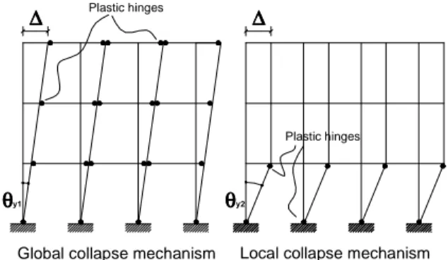
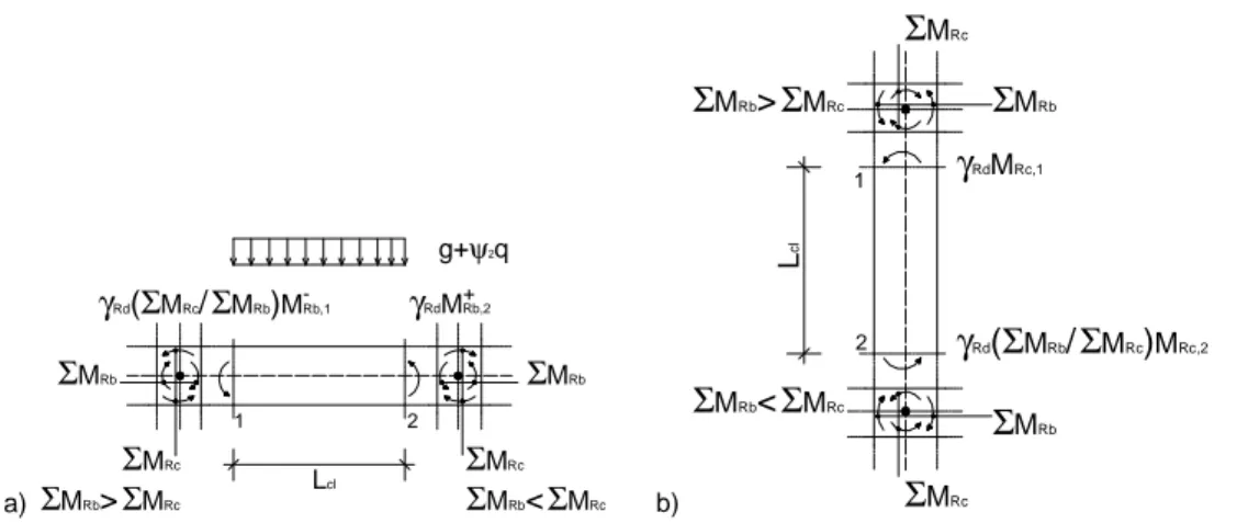
The capacity design approach was adopted, localizing plastic hinges in correspondence of the ends of the elements (both beams and columns), in order to achieve the development of ductile global collapse mechanisms instead of local brittle ones (figure 4.9). The shear design forces were defined considering the localization of flexural plastic hinges at the ends of the elements, according to the schemes presented in figure 4.10, taken from EN 1998-1:2005 [1].

Figure 4. 9: Global collapse mechanism vs local brittle ones (soft storey).

θθθθy1

∆∆∆∆ ∆∆∆∆

θθθθy2

Global collapse mechanism Local collapse mechanism

Plastic hinges

(12)

a) b)

Figure 4. 10: Determination of the design shear action (EN 1998-1:2005) for a) beams, b) columns.

The expressions used for the determination of the shear strenght, on the other hand, are the same generally used for buildings not in seismic areas (Eqn. 4.9), as presented in EN 1992-1-1:2005 [6], in which VRd is the design shear resistance for

the selected element, VRd,S the shear resistance due to steel stirrups, VRd,C the

shear resistance due to compression strut, α the angle between shear reinforcement and the beam axis perpendicular to the shear force, θ the angle between the concrete compression strut and the beam axis perpendicular to the shear force, bw the minimum width between tension and compression chords, z the

inner lever arm, Asw the cross-sectional area of the shear reinforcement, s the

spacing of the stirrups, fywd the design yield strength of the shear reinforcement, ν1

a strength reduction factor for concrete cracked in shear and αcw a coefficient

taking account the stress condition in the compression chord.

[

]

(

)

(

cot cot

)

/

(

1 cot

)

sin cot cot ; min 2 1 max , , max , , θ α θ υ α α α θ + + = + = = cd w cw Rd ywd sw s Rd Rd s Rd Rd f z b V f z s A V V V V (4.9)

The design of beams and columns was optimized in order to achieve sections with the minimum requirement of reinforcements: one of the main aims of the design was, in fact, the maximization of the ductility requirements imposed by seismic action to the rebar. As a consequence, steel bars of different diameters were used for longitudinal reinforcements, varying from 14 to 18 mm in both beams and columns.

As regards transversal reinforcements, stirrups of diameter 8.0 mm and 10 mm were generally used, respectively in beams and columns; in particular, rectangular double stirrups with four branches were often used in columns of the first and of the second floor, while simple rectangular stirrups were always used in beams. The spacing of stirrups generally varies from 50 mm to 100 mm in correspondence of the critical zones of beams and columns. The length of the critical zones of elements is defined according to what presented in EN 1998-1:2005 [1].

1 2 ΣMRb ΣMRc ΣMRb g+ψ2q ΣMRc γRd(ΣMRc/ΣMRb)MRb,1- γRdMRb,2+ Lcl ΣMRb<ΣMRc ΣMRb>ΣMRc

Σ

MRc

Σ

MRb

γ

RdMRc,1 1 2

γ

Rd(

Σ

MRb/

Σ

MRc)MRc,2

Σ

MRb>

Σ

MRc

Σ

MRb<

Σ

MRc

Σ

MRc

Σ

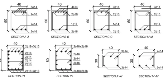
MRb L c l

(13)

Tables from 4.12 to 4.15 summarize the geometrical characteristics of structural elements of the different buildings selected as case studies, while figures from 4.11 to 4.21 present the structural details of reinforcements in beams’ and columns’ sections.

Residential building in HDC

Table 4. 12: Dimensions of structural elements for residential building in HDC. Residential building HDC

Floor Columns [cm x cm] Beams [cm x cm] Concrete Class Storey height [m]

1 40x70 40x50 C25/30 2,50

2 40x60 40x50 C25/30 3,00

3 40x50 40x50 C25/30 3,00

4 40x50 40x50 C25/30 3,00

5 40x50 40x50 C25/30 3,00

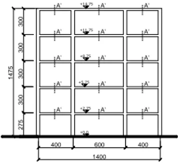
Figure 4. 11: Scheme of elements’ sections disposition for residential building in HCD (main frame).

Figure 4. 12: Elements’ sections disposition for residential building in HCD (secondary frame).

F C C B D D B C C A F F A C C B D D B C CA F FA C C B D D B C C AF F C C B D D B C C A F F A E E B E E B E EA F FA C C B D D B C C AF F D D B C C B D D A F F A D D B D D B D DA F FA D D B C C B D D AF F D D B C C B D D A F F A D D B D D B D DA F FA D D B C C B D C AF F D D B C C B D D A F F A D D B D D B D DA F FA D D B C C B D C AF P3 P3 P3 P2 P1 400 600 600 400 400 600 600 400 400 600 600 400 6000 +0.0 +2.75 +5.75 +8.75 +11.75 +14.75 3 0 0 3 0 0 3 0 0 3 0 0 2 7 5 1 4 7 5 600 400 3 0 0 3 0 0 3 0 0 3 0 0 2 7 5 400 1 4 7 5 1400 +0.0 +2.75 +5.75 +8.75 +11.75 +14.75 A' A' A' A' A' A' A' A' A' A' A' A' A' A' A'

(14)

Figure 4. 13: Typical sections of beam and column elements in residential building in HDC.

Residential building in LDC

Table 4. 13: Dimensions of structural elements for residential building in LDC. Residential building LDC

1 40x50 40x50 C25/30 2,50

2 40x50 40x50 C25/30 3,00

3 40x50 40x50 C25/30 3,00

4 40x50 40x50 C25/30 3,00

5 40x50 40x50 C25/30 3,00

Figure 4. 14: Scheme of elements’ sections disposition for residential building in LCD (main frame).

40 5 0 SECTION D-D 40 5 0 SECTION E-E 40 5 0 SECTION F-F 50 2 4 SECTION A'-A' 40 5 0 40 6 0 40 7 0 SECTION P3 SECTION P2 2φ16 2φ14 2φ16 2φ16 2φ14 2φ16 3φ14 2φ16 2φ14 2φ16 3φ14 2φ16 2φ14 2φ16 3φ14 2φ16 2φ14 2φ16 2φ14 2φ16 2φ16 2φ14 3φ14 3φ14 3φ18 2φ18 2φ16 2φ18 3φ18 3φ18 2φ18 2φ18 3φ18 3φ18 2φ18 3φ18 SECTION P1 40 5 0 2φ14 SECTION A-A 40 5 0 SECTION B-B 40 5 0 SECTION C-C 1 4 7 5 2 7 5 3 0 0 3 0 0 3 0 0 3 0 0 6000 400 600 600 400 400 600 600 400 400 600 600 400 M M P1 P2 P2 P2 P2 B BB BB B B C C B B B B B B C C B B B B B B B B AA A A A A B B A A B B A A B B A A A A A A B C BB BB B B C C B B B B B B C B B B B B B C C BB BB B B C C B B B B B B C B B B B B B C C CC C C C C C C C C C C C C C C C C C C C C C +0.0 +2.75 +5.75 +8.75 +11.75 +14.75

(15)

Figure 4. 15: Elements’ sections disposition for residential building in LCD (secondary frame).

Figure 4. 16: Typical sections of beam and column elements in residential building in LDC.

1 4 7 5 2 7 5 3 0 0 3 0 0 3 0 0 3 0 0 1400 400 600 400 A'M' A' A' M' A' A'M'A' A'M' A' A' M' A' A'M'A' A'M' A' A' M' A' A'M'A' M' A' A' A' A' A' M' M' A' A'M' A' A' M' A' A'M'A' 5 0 5 0 SECTION P2 40 5 0 2φ18+3φ16 2φ18+3φ16 2φ16 2φ14 2φ14 2φ16 SECTION P1 2φ14 2φ16 5φ14 2φ16 2φ14 2φ16 4φ14 2φ16 1φ14 2φ16 3φ14 2φ16 1φ14 2φ16 3φ14 2φ16 2φ14 2φ16 2φ14 3φ14 2φ14 2φ18+2φ16 2φ18+2φ16 2φ16 40 SECTION M'-M' 40 3 0 3 0 40 5 0 40 5 0 40 5 0 40 40

SECTION A-A SECTION B-B SECTION C-C SECTION M-M

3φ14

(16)

Commercial building in HDC

Table 4. 14: Dimensions and height of structural elements Commercial building HDC

Floor Columns [cm x cm] Beams [cm x cm]

1 40x80 40x60

2 40x70 40x60

3 40x60 40x60

4 40x60 40x60

5 40x60 40x60

Figure 4. 17: Elements’ sections for commercial building (

Figure 4. 18: Typical sections of beam and

2φ 8 2φ18 2φ18 40 6 0 40 6 0 6 0

SECTION M-M SECTION B-B SECTION C-C

40 8 0 40 7 0 2φ 8 2φ18 2φ18 2φ18+2 2φ16 2φ16 2φ16 2φ18+2 2φ18+2φ16 2φ18+2φ16 2φ16 2φ16 2φ16 2φ16

SECTION C (column) SECTION B (column)

Dimensions and height of structural elements for commercial building in HDC. Commercial building HDC

Beams [cm x cm] Concrete Class Storey height [m]

C25/30 5,00

C25/30 3,50

lements’ sections for commercial building (main frame yz, secondary frame xz).

cal sections of beam and column elements in commercial building in HDC.

40 40 6 0 SECTION C-C SECTION D-D 40 6 0 40 5 0 2φ18 SECTION E-E 1φ16 40 5 0 SECTION F-F 2φ 8 2φ18 2φ18 2φ16 2φ 8 2φ18 2φ18 1φ16 1φ16 2φ18 2φ 8 2φ18 2φ 8 2φ18 18+2φ16 16 16 16 18+2φ16 2φ18+2φ16 2φ16 2φ16 2φ18+2φ16

(17)

Office building in HDC

Table 4. 15: Dimensions of structural elements for office building in HDC. Office building HDC

1 40x80 40x60 C25/30 5,00

2 40x70 40x60 C25/30 3,50

3 40x60 40x60 C25/30 3,50

4 40x60 40x60 C25/30 3,50

5 40x60 40x60 C25/30 3,50

Figure 4. 19: Scheme of elements’ sections disposition for office building in HCD (main frame).

Figure 4. 20: Scheme of elements’ sections disposition for office building in HCD (secondary frame).

P1 P2 P3 P3 P3 D D A A A A A A A D A DD A DD A DD A DD A DDA DD A DD A DD A A A B A B A B B C C B B B B B B C C B B B A A A A A A A A A BB A B B A C C AB B A B B A B B A C C AB B A BB A BB A CC A BB A BB A BBA CC A BB A BB A A A A DD A B B A C C AB B A B B A B B A C C A B B A BB A BB A CC A BB A BB A BBA CC A DD A BB A A A A DD A D D D D D D D D D D D D D 10800 600 700 500 500 700 700 500 500 700 700 500 500 700 700 500 500 700 600 1 9 0 0 5 0 0 3 5 0 3 5 0 3 5 0 3 5 0 A A BB A B B A C C AB B A B B A B B A C C A B B A B A B A B A B B C C B B B B B B C C B B B A A A A A A A A A BB A B B A C C AB B A B B A B B A C C AB B A B A' A' A' A' A'A' A' A' A' A'A' A' A' A' A' A' A'A' A' A' A' A' A'A' A' A' A' A'A' A' A' A' A' A' A'A' A' A' A' A' A'A' A' A' A' A'A' A' A' A' A' A' A'A' A' A' A' A' A'A' A' 3000 400 700 400 400 700 400 1 9 0 0 5 0 0 3 5 0 3 5 0 3 5 0 3 5 0 A' A'A' A' A' A' A' A' A'A' A' A' A' A' A'A' A' A' A' A'A' A' A' A' A' A' A'A' A' 40 6 0 3φ18 2φ8 2φ18 SECTION A-A 40 6 0 4φ18 2φ16 2φ16 4φ18 SECTION B-B 40 6 0 2φ18 2φ8 3φ18 SECTION C-C 40 6 0 5φ18 1φ16 2φ8 3φ18 SECTION D-D 40 8 0 4φ18 2φ16 2φ16 2φ16 4φ18 4φ18 2φ16 2φ16 4φ18 5φ18 2φ16 2φ8 3φ18 1φ16 40 7 0 40 6 0

(18)

4.3 Backgrounds for the elaborations of non linear models

Non linear two-dimensional models were elaborated for each of the two main directions of designed case studies using OpenSees software [75].

Beams and columns were modelled as beam with hinge (BWH) elements: each single element was divided into three different portions, two plastic hinges in correspondence of the two ends and an elastic central part (figure 4.22.b). The definition of the section in correspondence of the central part of the element required only the individuation of the transversal area (A) and of the elastic modulus of material (Em); on the other hand, the sections in correspondence of the

two ends of beams and columns were modeled as “fiber sections” and an opportune length (Lp) for plastic hinges was defined, based on the definition

proposed by Fardis [77] for cyclic loading condition (equation 4.10).

Columns were considered fixed in correspondence of the base and seismic masses were concentrated in correspondence of the top of the columns, as well as vertical loads. In order to reproduce the stiffening contribution of storey slab, additional truss elements, opportunely sized, were introduced in the model between column elements (figure 4.22a).

a) b)

Figure 4. 22: a) Simplified scheme of non linear models, b) BWH element.

The selection of opportune constitutive laws for both concrete and steel materials was necessary in order to provide significative and reliable results for the deformation levels obtained in reinforcements.

For concrete material, the constitutive law proposed by Braga, Gigliotti and Laterza [79] was used, in order to directly represent the confinement contributions due to both longitudinal and transversal reinforcements; the BGL model was recently implemented in OpenSees (D’Amato [72]) considering different possible layouts of transversal stirrups (figure 4.23).

Figure 4. 23: Different stirrups layout for Braga, Gigliotti and Laterza [79] confinement model.

For steel reinforcing bars, the modified slip model presented in the previous paragraphs was adopted, allowing to consider the relative slip phenomena

3 0 0 3 0 0 3 0 0 3 0 0 1 4 5 0 2 5 0 400 600 600 400 400 600 600 400 400 600 600 400 6000 Plastic hinge on beams Plastic hinge on columns x z

truss elements for storey slab

Plastic hinge

Plastic hinge Elastic central part (E,A) Lp Lp s1 s2 s3 s4 C R

(19)

between steel reinforcements and concrete according to what presented in Chapter 3. Different coordinates, in terms of axial stress-slip and axial stress-fictitious strain, were derived in relation to the different bar diameters used in the design for beams and columns; the modified slip model was implemented in OpenSees [75] using the trilinear hysteretic material, with the three characteristic points of the loading envelopes opportunely determined in relation to the energy equivalence principle (figure 4.24).

Figure 4. 24: Shift from axial stress-slip model to axial stress-fictitious strain model for steel bars.

For the modified slip model, the following hypothesis were adopted:

• The constitutive stress-strain relationship of steel was assumed elastic-plastic with hardening (figure 4.25); the values adopted for yielding and tensile strenght and for the elongation to maximum load were calibrated in relation to the mean values of the experimental tests’ results presented in Chapter 2 for the corresponding steel grade used in the design (B450C).

Table 4. 16: Mean values of experimental test on B450C-TempCore bars and values for the model.

B450C – TempCore steel fu [MPa] fy [MPa] fu/fy [-] A[%] Agt [%]

Mean (Experimental test) 596.60 488.00 1.22 26.40 14.10

Assumed for model 600.00 490.00 1.22 26.40 14.00

Figure 4. 25: Simplified stress-strain relationship assumed for steel constitutive law.

• The bond stress-slip relationship was assumed elasto-plastic (figure 4.26), in agreement with what already presented by Braga et al. [70]. In particular, the simplification adopted in the slip model was extended to the case of ribbed bars

A x ia l s tr e s s , σ Deformation, ε (ε1p,σ1p) (ε2p,σ2p) (ε3p,σ3p) (ε1n,σ1n) (ε2n,σ2n) (ε3n,σ3n) 0 k0 A x ia l s tr e s s , σ Axial slip, u A B C Y U ES Eh A x ia l s tr e s s , σ Axial Strain, ε fu fy εy εp _A_gt

Real stress-strain diagram

(20)

concrete due to cycling actions, the residual bond stress to use in the model (τd)

was taken equal to the one prescribed for poor bond conditions in confined concrete. For u1 the value obtained from the intersection between the residual

bond stress and the linear approximation of the first branch of the Model Code relationship was assumed.

Table 4. 17: Assumed values for the bond stress-slip relationship in modified slip model. Confined concrete - All other bond condition

Model Code 90 Assumed values for modified slip model

s1 [mm] 1.0 sb [mm] 0.4

s2 [mm] 3.0 s2 [mm] -

s3 [mm] Clear rib spacing s3 [mm] -

α 0.4 fck [MPa] 33

τmax [MPa] 1.25√fck τmax [MPa] 7.18

τf [MPa] 0.40τmax τf [MPa] 2.87

Figure 4. 26: Bond stress-slip relationship assumed for the modified slip model.

• The axial stress-strain to be used in the numerical models was obtained as already presented in Chapter 3, according to what provided by D’Amato [72]; a fictitious strain ε* was individuated through equation (3.98), in which the plastic hinge length Lp was defined according to Panagiotakos and Fardis [78], as

presented in equation 4.10: P tot L

L

u

_, *

₌

ε

y b sl s cy pl L a d f L _, =0.12⋅ +0.014 (4.10)

Being Ls the shear span length, asl a coefficient for slip equal to 1 if there is

slippage of the longitudinal bars from their anchorage beyond the section of maximum moment, or to 0 if there is not slip, db is the bar diameter and fy the

yielding strength. In the present work, the value of asl was assumed equal to

zero, since the relative slip phenomena between bars and the surrounding concrete was directly taken into consideration in the modified slip model.

B o n d s tr e s s , τ Slip, s τmax τf s1 s2 s3 Confined concrete (MC90)

other bond condition

sb

Assumed model Linearization of the first branch

(21)

a) b)

Figure 4. 27: Bond stress-slip relationship and trilinear equivalent model. Table 4. 18: Assumed values for the axial stress-slip model Mechanical properties of material

Axial stress-slip relationships: coordinates of significative points

fy 490 MPa

fu 600 MPa d 14 mm d 16 mm d 18 mm

εy 0.24 % up1 0.400 mm up1 0.400 mm up1 0.400 mm

Agt 12.50 % σp1 318.56 MPa σp1 297.80 MPa σp1 280.77 MPa

Es 206000 MPa up2 0.743 mm up2 0.839 mm up2 0.936 mm

Eh 1047.00 MPa σp2 517.30 MPa σp2 517.44 MPa σp2 517.59 MPa

τd 2.87 MPa up3 11.475 mm up3 13.104 mm up3 14.734 mm

u1 0.4 Mm σp3 600.00 MPa σp3 600.00 MPa σp3 600.00 MPa

0 100 200 300 400 500 600 700 0 3 6 9 12 15 A x ia l s tr e s s [ M P a ] Slip [mm] diameter 18 mm diameter 16 mm diameter 14 mm 0 100 200 300 400 500 600 700 0 3 6 9 12 15 A x ia l s tr e s s [ M P a ] Slip [mm] Trilinear 18 mm Trilinear 16 mm Trilinear 14 mm