5 STIFFNESS CHAIN EVALUATION OF THE SETUP 5.1 Introduction

5

STIFFNESS CHAIN EVALUATION OF THE SETUP

5.1

Introduction

In this chapter will be analyzed the static stiffness behaviour of the machine’s components. From the literature [13] it has been noticed that the most used hypothesis when evaluating micromilling is that the biggest component of compliance originates from the tool, due to its high slenderness. However, in [14] the results contradict this hypothesis on the conventional scale and it means that the stiffness chain of the whole system needs to be determined. In order to evaluate the stiffness chain of the setup at TU Delft, an existing evaluation method has been chosen and tailored according to the characteristics of micromilling.

The general approach is to evaluate the stiffness of each element on this setup separately, modelling it as a spring, and assessing it via experimental testing, which consists of applying a known load and measuring the ensuing deformation at same place. This means that each element in the system is measured with specially designed measuring methods. Fig. 5.1Fig. 5.1 shows the compliance links taken into account.

Fig. 5.1- Micro-milling machine’s components

Fig. 5.2- Equivalent stiffness chain of all machine’s components

KX-STAGE

KY-STAGE

KY-CONNECTION

KZ-SPINDLE CONNECTION

KBRIDGE KZ-STAGE KSPINDLE KTOOL KX-CONNECTION

As it can be seen, these springs are connected in a serial way. When summing up these stiffness in order to get the global stiffness of the machine, there is a rule to follow:

1/k1 + 1/k2 + ... + 1/kn = 1/kreplace (5.1)

In order to know the importance of every elastic element shown in Fig. 5.2, an explanation of them follows:

• KBASEMENT : considering the dimension and the granite basement, it is possible to assume it as

infinitive rigid. It is the “fixed world” respects to all the other related components.

• KBRIDGE: the bridge is a granite construction too and it connects the table with the Z stage

with a defined distance.

• KZCONNECTION: represents the connection between the bridge and the z-stage; in order to get

an idea of the stiffness of this connection, a short calculation [Appendix E] has been made.

• KZ_STAGE: represents the stiffness of the Z-stage, that it is a very important component for the

deflection of the tool.

• Kspindle_connection : is the connection between the spindle and the Z-stage. Given that there is a

short distance from the endmill tip and the spindle and the connection points are far from each other, no problems are expected.

• KSPINDLE : the stiffness of the spindle that will be later evaluated.

• KTOOL_HOLDER: the stiffness of the tool-holder that will be evaluated with an experimental set

up, together with the stiffness of spindle, Z-stage and bridge.

• KTOOL: the stiffness of different kinds of tools (in diameter and shape) that will be evaluated

later via experimental testing.

• KCONNECTIONX: is the connection of the X-stage to the table. The stage can only be connected

to the table with bolts screwed inside it. The same calculation can be use with KZCONNECTION.

• KX_STAGE e KY_STAGE: these will be evaluated together, as a unique elastic element, via

experimental testing.

• KCONNECTIONY: is the stiffness of the connection between X and Y stages.

The springs relative to the X and Y stages are linked to the chain through the workpiece. It is not included in the chain and is here considered as an infinitive rigid element that transfers the force totally from the tool to the Y-stage. In fact it was not possible to consider its stiffness, because of the great variety of material that will be used during the micro-milling operation.

In the rest of the chapter the different experimental tests made to evaluate the stiffness of each component are analyzed.

Considering that every experiment is affected by errors, some corrective factors have been found and considered in the final value. The global compliance of the whole chain has been found and it represents the upper limit of the compliance range.

5.2

Tool stiffness

5.2.1 Design of method

For a first approach, the tool as a cylindrical cantilever beam has been considered. The deflection will be conform to the equation 5.2:

x MAX EI Fl 3 3 =

δ

where: δmax is the maximum displacement under the force application point;

F is the applied force; E is the Young module;

Ix is the inertia moment of the beam.

The geometry of the tool is (Fig. 5.3):

Fig. 5.3-Geometry of the tool

where dT is the equivalent diameter of the cutting part (it is considered as first hypothesis the

80% of the nominal value d in order to introduce the effect of the flute shape [13]), l is the length of the cutting part, dy is the diameter of the transition part evaluated finding its centre of mass and the

diameter at that point and its length c is evaluated knowing the conic angle β measured during the experimental test. D is the diameter of the shank part length p.

The tables show, respectively, the values of the geometrical parameters of the tool (Tab. 5.1) and the material’s characteristics (Tab. 5.2).

dT

D

shank Transition part Cutting part

p c l

dy

Tool label D[µm] d[µm] dT[µm] dy[µm] p[µm] c[µm] l[µm] α[°] Cuttin g edges numbe r 0.3_10 6,00E+ 03 3,00E+ 02 2,40E+ 02 4,03E+ 03 2,04E+ 04 1,80E+ 04 6,00E+ 02 9,00E+ 00 2 0.3_11 6,00E+ 03 3,00E+ 02 2,40E+ 02 4,03E+ 03 2,04E+ 04 1,80E+ 04 6,00E+ 02 9,00E+ 00 2 0.5_VHMS-2005_1 6,00E+ 03 5,00E+ 02 4,00E+ 02 4,26E+ 03 2,24E+ 04 1,56E+ 04 1,00E+ 03 1,00E+ 01 2 0.5_SPMS-2005_1 6,00E+ 03 5,00E+ 02 4,00E+ 02 5,05E+ 03 2,95E+ 04 8,46E+ 03 1,00E+ 03 1,80E+ 01 2 0.5_SPMS-2005_2 6,00E+ 03 5,00E+ 02 4,00E+ 02 5,05E+ 03 2,95E+ 04 8,46E+ 03 1,00E+ 03 1,80E+ 01 2 0.5_SPMS-4005_1 6,00E+ 03 5,00E+ 02 4,00E+ 02 5,05E+ 03 2,95E+ 04 8,46E+ 03 1,00E+ 03 1,80E+ 01 4 0.5_SPMS-4005_2 6,00E+ 03 5,00E+ 02 4,00E+ 02 5,05E+ 03 2,95E+ 04 8,46E+ 03 1,00E+ 03 1,80E+ 01 4 Tungsten Carbide Elastic Modulus 560000 [N/mm2] Poisson Ratio 0.22 Shear Modulus 220000 [N/mm2] Thermal Expansion Coefficient 5,00E-06 Density 0.0136 [g/mm3] Thermal Conductivity 88 [W/kg °K] Specific Heat 220 [J/kg °K] Tensile Strength 1440 [N/mm2] Yield Strength (Transverse rupture strength) 4200 [N/mm2]

Tab. 5.2 Material’s characteristics of the tool

In order to evaluate the static stiffness of the tool (Fig. 5.4) three different analyses have been made: a theoretical, a FEM and an experimental analysis.

In each of them the stiffness is evaluated as the ratio between the force applied at tool tip and the displacement at the same point in the direction of perpendicular to the tool axis.

Fig. 5.4 – Micro-milling tool.

5.2.1.1 Theoretical analysis

There are two main reasons for analyzing the tool with a theoretical model:

• to provide an estimation of the value of the tool.

• to use this value to correct the experimental stiffness results. It is in fact necessary to link two cases: the one with the force applied not exactly at the free end of the tool and the displacement at the tool tip, with the one with the force and the corresponding displacement applied at the free end of the tool. This is due to the fact that during the experimental testing it is very difficult to apply the force exactly at the tool tip. So an interpolation to transfer the force to the same point where the displacement is calculated is necessary. This will be the interpolation factor α.

Two different kinds of model have been considered to estimate the theoretical value of the tool stiffness:

1. one cylindrical section cantilever beam model; 2. three sections cantilever beam model.

Fig. 5.5 – One cylindrical section cantilever beam model of the tool

5.2.1.1.1 One cylindrical section cantilever beam model

In this model (Fig. 5.5) the shank part, with the biggest diameter (D), is assumed to be infinitely rigid compared with the cutting part (dT). For that reason only the cutting part of the tool length l is

going to be analyzed.

For this introductive calculation also the force is considered applied perfectly at the tool-tip, although it is not possible to obtain in experimental tests. Afterwards the force is transferred at the tool-tip through an interpolation of the value evaluated in the real application point.

The final part is modelled as a cantilever beam perfectly clamped at point B. The displacement

us in a longitudinal direction is evaluated with the Elastic Line Method, as a function of the axial

coordinate s. The function us depends on the force application point.

s us B l dT F δMAX Y X

4 64 T x d I =

π

Integrating twice the equation 5.4, and considering the boundary condition, it is possible to find the us function:      ≤ ≤       − = l s s ls EI F u x s 0 6 2 3 2 (5.5)

In order to use this analysis to correlate the experimental stiffness results, it is necessary to evaluate the value of the interpolation factor α. To do that it is opportune to consider both the different cases: the first is an ideal case (Fig. 5.6 up), with the force applied to the tool tip and the displacement measured at the same point; the second is the real case (Fig. 5.6 down), with the force applied at the real application point, distant r from the tool tip and the displacement measured under the tool tip.

In order to link the two cases, it is necessary to equal the two maximum displacements δmax1 and

δmax2; by doing this, it is possible to find the value of the force F1 applied on the tool tip, which can

give a displacement of the same magnitude of the one that has effectively been measured.

Fig. 5.6-Ideal and real case of the force application point

2 max 1 max

δ

δ

(

)

α

Where: F1 is the force applied on the tool tip in the ideal case;

F2 is the force applied on a distance r from the tool tip, in the real case;

L is the distance between the clamping point and the force application point in the real F1 δmax1 s F2 δmax2 s L r

case;

So it is possible to calculate the stiffness value KTOOL as:

2 max 2 1 max 1

δ

α

δ

and compare it with the theoretical value of the stiffness Kth=F1/δmax1.

Fig. 5.7 – Three section beam tool model (up). Conic part of the model (down)

5.2.1.1.2 Three sections beam model

In order to have a more accurate theoretical analysis, a three section beam model, which better represents the real shape of the tool, has been made (Fig. 5.7). The length of the shank part a is considered related with the position of the tool in the clamping system, during the experimental test.

4 1 64D I =

π

π

π

Where: I1 is the inertia moment of the shank part;

I2 is the inertia moment of the transition part;

I3 is the inertia moment of the cutting part;

H is the free bending length.

For this calculation the two different cases are also compared (Fig. 5.6). A relationship between the force at the tool tip and the force at the experimental point has been found, in order to compare the theoretical and experimental results, as before.

l dT c F D Tool a C s H 1 2 3 c B A Conic part dT Y X

The same elastic line method is applied at the new model, considering the displacement of the tip point as the sum of the displacement of the point A with the stiffness of the beam1, the displacement of the point B with the stiffness of the beam 2, and the displacement of the point C with the stiffness of the beam 3.

Equalling the two maximum displacements δMAX1 and δMAX2 (equation 5.13), the interpolation

factor has been obtained (equation 5.14).

2 max 1 max

δ

δ

(

)

(

)

(

)

α

Where F1, F2, L and r have the same meaning of the Fig. 5.6.

So it is possible to calculate the stiffness value KTOOL as:

2 max 2 1 max 1 δ α δ F F K_TOOL = = (5.15)

And compare it with the theoretical value of the stiffness Kth=F1/δmax1.

The Tab. 5.3 shows the values of the interpolation factor α evaluated with both the models. As it can be seen, the three sections beam model is more accurate than the other, and the interpolation factors are bigger. So in the analysis below it has been considered the three sections beam model.

5.2.1.2 FEM analysis

There are two main reasons for analyzing the tool with a finite elements model (FEM):

• to provide an estimation of the value of the tool stiffness, therefore to know the qualitative behaviour of it;

• to verify the hypothesis of 80% of the value of the nominal diameter for the diameter of the cutting part.

The finite element analysis has been done using the Solid Works software with 3D elements. It has been done only for the 0,5mm diameter endmill.

Tool label Interpolation Factor Three Sections Beam Model Interpolation Factor One Section Beam Model 0.3_10 2,72E-01 2,57E-02 0.3_11 2,70E-01 2,26E-02 0.5_VHMS-2005_1 8,28E-01 3,45E-01 0.5_SPMS-2005_1 7,48E-01 3,72E-01 0.5_SPMS-2005_2 7,67E-01 4,23E-01 0.5_SPMS-4005_1 8,32E-01 5,49E-01 0.5_SPMS-4005_2 8,68E-01 5,11E-01

Tab. 5.3-Interpolation factors of the two models

. Cutting part cross

section area [mm2] Nominal area [mm2] Ratio Equivalent cutting part radius [mm] equivalent circle diameter [mm] 0.5_VHM S -2005 0.1384 0.1964 0.7051 0.2099 0.4198 0.5_SPM S-2005 0.1514 0.1964 0.7709 0.2195 0.4390 0.5_SPM S-4005 0.1534 0.1964 0.7813 0.2210 0.442

Tab. 5.4 -Equivalent diameters for the 0.5 mm tool from the FEM analysis

The cutting part area is simulated by a circle with the equivalent diameter, which is calculated by the area ratio between the real tool cross section and the nominal tool cutting radius (0,25mm). The values are listed in Tab. 5.4.

In order to use more accurate value of the equivalent diameter in the theoretical analysis, the ratio found with the FEM analysis, which consider the real shape of the flute and the cutting edge’s number, has been used. The tab. 5.5 shows the results of the FEM analysis made for three means of tools. The model of the tool is displayed in

Fig. 5.8.

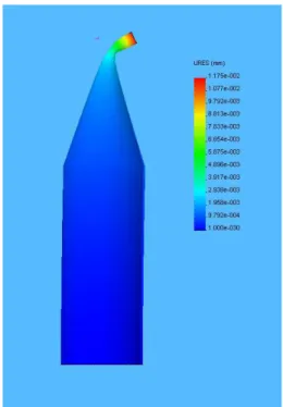
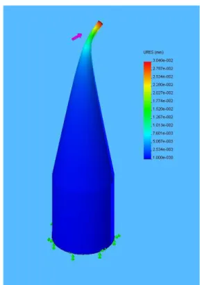
The tool is constrained on the bottom side in all directions. The force is applied on the tool tip as shown in Fig. 5.9, and it has a magnitude of 15N. This force is comparable with the cutting force during micromilling experiments. Fig. 5.10 , Fig. 5.11 and Fig. 5.12 show the results of the FEM analysis for each kind of tool.

FEM simulation [N/µm] 0.5_VHMS -2005 0.4934 0.5_SPMS-2005 1.266 0.5_SPMS-4005 1.277

Tab. 5.5-FEM analysis results

Fig. 5.8-Tool’s model in the FEM analysis

Fig. 5.10-0.5_SPMS -2005 tool, FEM results

Fig. 5.12-0.5_VHMS -2005 tool, FEM result

5.2.1.3 Experimental set-up

To calculate the experimental value of the tool stiffness is necessary to measure the displacement at the tool tip when a perpendicular force is applied, when clamping the tool on the shank part.

For clamping the tool, the different systems that can be used are:

• mechanical clamping system,

• hydraulic clamping system,

• magnetic clamping system

Due to the small dimension of the tool and the relatively low force that is going to be applied, a mechanical clamping system has been chosen. Given that in the laboratory there was no available system, a new one has been designed. It gives the possibility to adjust the height of the tool, so it has been used for all the tools tested.

Concerning to the load, a device to apply the force as close as possible to the tool tip is needed. The different systems that can be used are:

• wire with calibrated weights,

• an inclined plane touching the tip, with some calibrated weights on it;

• a dynamometer.

Due both to the small load to apply (at most 10N with a 1mm tool’s diameter), and the small dimension of the tool tip, a wire with calibrated weights has been chosen, also because it is a very simple method to use.

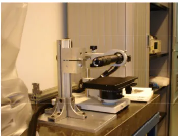
Fig. 5.13- Experimental set-up: tool clamping system and microscope lens

Finally there is the choice of the instrument for measuring the displacement. From the literature [13, 14] and the theoretical and FEM analyses it is known the expected value of the tool stiffness, so it is possible to calculate an expected displacement for each tool under test.

Given that the estimated displacement is on the order of micrometer, an instrument with a proper resolution, at least 0,1µm is necessary.

The several instruments that can be used are:

• dial devices, resolution 1µm,

• inductive or capacitance sensor, resolution less than 1µm,

• laser sensor, resolution of 0,01µm,

• Keyence microscope, resolution depending on the resolution.

Concerning to the dial devices, there are several problems depending on this measuring procedure, due to both the contact point of the probe with the tool and the skill of the worker that is performing the measurements [14].

About the use of the sensors, the problem depending on their use is that the surface measured at the tool tip is not a flat surface, so it is difficult to position the spot of the sensor exactly in the tip point, due also to the small diameter of the tested tools.

For these reasons the Keyonce Microscope has been chosen.

The method designed to analyze the experimental stiffness of the tool consists of clamping the tools with a mechanical clamping system, designed properly for that, and loading the tool tip in a vertical plane, using a weight hung on a different diameters wire. This configuration enables the assumption made that the tool is perfectly clamped at the cylindrical part, since it is secured in this case by a highly rigid device (Fig. 5.13).

Before starting to collect the data, some tests have been made to rely on the set-up and to check if it is stiff enough. In fact in the first set of measurements just touching the clamping system a displacement could be seen. So using mechanical devices the whole set-up has been made stiffer.

The tool was loaded using a fishing wire of 0,07mm in diameter and calibrated weights of 100g and 50g, with a weight hung of 100g. A maximum of 10N was applied. Several kinds of wire were tried: the found problems are due to the relative big dimension of the wire respect to the tool tip diameter, and the maximum load of the wire. One of the most delicate points in making these tests was fixing the wire as close as possible to the tool tip. Finally it has been fixed at a distance that is

in a range between 114,75µm and 618,50µm from the tip. This arrangement was used to theoretically obtain the tool deflection, assuming that the load was applied at the very tip (Fig. 5.14).

Fig. 5.14- Experimental set-up. Tool under load, with the camera focus on it

Given that two different diameter tools have been tested, an optical camera with different magnifications has been used, and at the end it has been chosen a 1000X magnification for the ø 0,5mm tool and a 200X magnification for the other diameter. The image has been displayed on a colour monitor. This test bed configuration enabled the tip of the tool centred on the monitor under no load. Then the tool tip wire was loaded and both the displacement of the tip from the point of reference and the distance of the wire were measured. The tests comprised two load cycles for each tool, and two identical tools for each kind of them.

5.2.2 Experimental Results

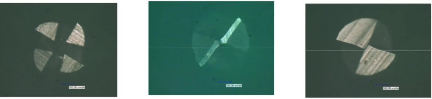
5.2.2.1 Ø 0.3 mm tool

The results of the ø 0,3mm tool (Fig. 5.15) have been obtained with loads from 0 to 5N, and the corresponding displacements varied from 0µm to a range between 21,04 and 23,14µm. The behaviour of the tool is linear as shown in Fig. 5.16, and the straight line fitted to the experimental results shows an experimental static stiffness of Kexp_0.3 =0,21~0,23N/µm.

The load was not applying precisely at the tool, thus it is necessary to transfer the force at the free end, the application point of the cutting force, using the interpolation factor. Given the values of the interpolation factors α, the stiffness value of the tool at the tool tip has been

Kt_0.3=0,052~0,056N/µm.

Fig. 5.15-ø0.3 mm tool stiffness Fig. 5.16- ø 0.3 mm diameter tool

tool 0,3_10 y = 0,0562x - 0,0059 R2 = 0,9919 0,0 0,2 0,4 0,6 0,8 1,0 1,2 1,4 1,6 0,0 2,0 4,0 6,0 8,0 10,0 12,0 14,0 16,0 18,0 20,0 22,0 24,0 displacement [um] fo rc e [ N ]

Fig. 5.17- ø0,5mm VHMS-2005 Fig. 5.18- ø 0,5mm SPMS-2005 Fig. 5.19-ø 0,5 mm SPMS-4005

5.2.2.2 Ø 0.5 mm tool

The results of the ø 0,5mm tool were obtained with different loads, a cycle load between 0N and 5N for the VHMS-2005 tool, between 0N and 2N for the SPMS-2005 tool, and SPMS-4005 tool. Three different types of 0.5mm diameter have been tested, and the results are listed below:

• Ø 0,5mm VHMS-2005- two cutting edge tool (Fig. 5.17): the obtained displacement varied from 0µm to a range of 11,57 ~12,62µm, the experimental static stiffness has been

Kexp_0.5VHMS_2005 =0,38~0,42N/µm., the stiffness value at the tool tip has been Kt_0.5VHMS_2005=0,31~0,34N/µm;

• Ø 0,5mm SPMS-2005- two cutting edge tool (Fig. 5.18): the obtained displacement varied from 0µm to a range of 2,56 ~ 2,61µm, the experimental static stiffness is

Kexp_0.5SPMS_2005 =0,75~0,76N/µm., the stiffness value at the tool tip is Kt_0.5SPMS_2005=0,56

~0,58N/µm;

• Ø 0,5mm SPMS-4005- four cutting edge tool (Fig. 5.19): the obtained displacement varied from 0µm to a range of 2,43 ~ 2,54µm, the experimental static stiffness is

Kexp_0.5SPMS_4005 =0,80~0,77N/µm., the stiffness value at the tool tip is Kt_0.5SPMS_4005=0,67

N/µm.

5.2.2.3 Ø 1.0 mm tool

The paragraph below includes the results of the ø 1,0mm (Fig. 5.21) tests just for completeness, but it is not going to be analyzed and compared with the others, because it has been tested with different kind of set-up.

The wire used in this case has been a ø 0,4mm with a cycle load between 0N and 10N. The corresponding displacements varied from 0 to a range between 15,78 and 17,88µm. The behaviour of the tool is linear as shown in Fig. 5.20, and the straight line fitted to the experimental results shows an experimental static stiffness of Kexp_1.0 =0,55~0,62N/µm.

Considering that the load was not applying precisely at the tool tip, the next step was to obtain the stiffness of the tool when the force was applied at the free end, similarly to the point of action of the cutting force. Given the values of the interpolation factors α, the stiffness value of the tool at the tool tip was Kt_1.0=0,38~0,44N/µm.

5.2.3 Conclusions and analysis of the results

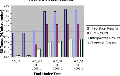
Table below summarizes the all found results:

As expected, the most stiff tool is the 0.5_SPMS-4005, with a value of

Kt_0.5SPMS_4005=0,68N/µm. For each kind of tool, three specimens have been tested and the values of

the stiffness have been obtained. These results are coherent with the shape of the tools, in fact the differences with the others are due to two main reasons:

Fig. 5.20-ø1.0 mm diameter tool Fig. 5.21- ø1.0 mm tool stiffness Tool label Theoretical Stiffness [N/µm] FEM Stiffness [N/µm] Experimental Stiffness [N/µm] Interpolation Factor Interpolated Stiffness [N/µm]

0.3_10 9,33E-01 / 2,10E-01 2,72E-01 5,71E-02

0.3_11 9,32E-01 / 2,30E-01 2,70E-01 6,20E-02

0.5_VHMS-2005_1 1,07E+00 4,90E-01 3,75E-01 8,28E-01 3,10E-01

0.5_SPMS-2005_1 1,78E+00 1,27E+00 7,47E-01 7,48E-01 5,59E-01

0.5_SPMS-2005_2 1,78E+00 1,27E+00 7,61E-01 7,67E-01 5,84E-01

0.5_SPMS-4005_1 1,87E+00 1,28E+00 8,02E-01 8,32E-01 6,68E-01

0.5_SPMS-4005_2 1,87E+00 1,28E+00 7,67E-01 8,68E-01 6,66E-01

Tab. 5.6-Summarizing of the tool’s results.

1. the shape of the transition part: the bigger is the conic angle the bigger is the equivalent

diameter of the conic part and the more stiff is the tool; for the SPMS tool the conic angle is double the one of the VHMS tool;

2. the number of the cutting edges: that influences the equivalent diameter of the cutting

part of the tool; if there are more cutting edges, the equivalent diameter is bigger and the tool is more stiff. Comparing the SPMS-4005 and the SPMS-2005 tools, a difference in terms of stiffness can be noticed, due to the increase of the number of the cutting edges: passing from 2 to 4 cutting edge, the stiffness rises of the 12% (Fig. 5.22, Fig. 5.23, Fig. 5.24)

By looking at the results, in order to achieve the best situation from a stiffness point of view, it could be better to have a conic angle as big as possible, given the diameter of the tool.

It can be easily noticed the difference between the theoretical, the FEM and the experimental values. The possible reasons for these differences can be:

• Concerning the FEM and theoretical analyses:

tool_1_5 y = 0,597x + 0,0975 R2 = 0,9931 0,0 2,0 4,0 6,0 8,0 10,0 12,0 0, 0 1, 0 2, 0 3, 0 4, 0 5, 0 6, 0 7, 0 8, 0 9, 0 10 ,0 11 ,0 12 ,0 13 ,0 14 ,0 15 ,0 16 ,0 17 ,0 18 ,0 displacement [um] fo rc e [ N ]

Fig. 5.22- cutting edge SPMS-4005 Fig. 5.23- cut. edge SPMS-2005 Fig. 5.24- cut. edge VHM-2005

1. the CAD drawing is a simplified geometry of the endmill, it includes all the key geometries, but it is not possible to draw some features from the manufacturing process, such as the flute mark;

2. the flute mark on the transition part has a negative influence on the endmill stiffness, which can not be taken into account in these analysis;

3. the influence of the manufacturing process: because of the unsharp of the grinding wheel and its wear out, the designed geometry cannot be manufactured exactly as the designed value, so the real tested tool is necessarily different from the nominal tool; the FEM and the theoretical analyses are used to study the endmill stiffness qualitatively. These give a good prediction of the stiffness change by optimizing the tool geometry, but they can not be taken as absolute values for the stiffness;

4. ;the fact that the theoretical and the FEM values are bigger than the experimental one is coherent with the studied literature [13, 14].

• Concerning the experimental results: all the sources of error that influence the final measure have been considered, in order to find some factors to correct the interpolated stiffness value. Starting from the experimental set-up, it is important to consider:

1. the stiffness of the clamping system of the tool: in the theoretical calculation it is considered as infinitive rigid, so it is necessary to be sure that the influence of its stiffness is negligible. In order to achieve it, it has been fixed with some stirrups directly to the granite table used for the experiments, and some tests with a known stiffness test piece have been made. It is found that the influence of the clamping system is about the 10% of the value of the tool stiffness Kt. So the corrective factor is fclamping_system= 0,90;

2. the stiffness of the microscope equipment: even if the tool is not physically linked with that, it influences the results during the displacement’s reading. To overcome this problem, the optical fibre cable of the microscope has been fixed on the table, and a fixture has been used to mount the lenses. Paying attention not to touch the cable during the measurements, it has been noticed that the influence of the microscope equipment is about the ±2% of the final value. So the corrective factor is fmicroscope_equipment= 0,98;

3. the characteristics of the wire used during the tests: for the experiments at the end a ø 0,07mm fishing wire has been used, that it was the thinnest wire available. For its characteristics, it can be considered as an ideal wire: no mass, perfectly elastic, without friction. So it can be assumed it transfers all the force applied on it to the tool. With these hypothesis it can be neglected the influence of it on the final result;

4. the position of the wire: even if during the experiments it has been tried to position the wire as close as possible to the tool tip, it has not been possible to achieve the tool tip in any case. In every tests the wire in different points was positioned, and it has been noticed that a variation of ±1mm in the distance between tool tip-force application point gives a variation of ±0,5% in the final value of the stiffness. So the corrective factor is

fwire_position=0,98;

5. the friction of the pulley: to apply the force, a fixture with a pulley system has been used. Considering the state of the pulley and how it has been done, it has been assumed as an ideal pulley, therefore without friction. Its influence on the final result is negligible. As regards the reading of the measurement, it is important to consider:

1. the position of the reference point: before to start the measurement a reference point has been chosen, in order to calculate the displacement of the tool. During the choice it has been considered that it was not much reliable to take as reference a point on the boundary of the wire, because the latter moves and changes position covering that point; 2. the lights and shadows crated by the microscope light: during the application of the

force, while the tool is deflecting, the light of the lens changes and creates shadows that confuse the measurement point.

Anyway the errors related with the measurement’s reading can be neglect if some expedients are taken, as to take the reference point on a cutting edge and to illuminate it in a correct way to avoid the problem of light and shadow. In conclusion the influence of the errors due to the measurement’s reading is negligible.

Finally it is to consider the source of error due to the interpolation of the experimental

value, to obtain the real value of the stiffness. In fact introducing it, an error due to the

theoretical calculation is introduced. In the present analysis it is measured the displacement at the tip of the tool, when a force is applied at a known distance from it. In order to find the correct value of the stiffness, that is the ratio between the applied force and the displacement under the force application point, the force is transferred to the tool tip. The error due to the theoretical calculation is here introduced. This procedure enables to minimize that error: in fact it is possible also to transfer, with another interpolation factor, the displacement under the force application point. However this procedure introduces a double error, due to the fact that it needs to use twice the theoretical formulas (in fact it needs both the theoretical value of the displacement under the force point and the theoretical value of the rotation of the section). Thus the influence of the error can be estimated as ±1% of the final value, given the approximation used in the theoretical calculation (0,01µm). So the corrective factor is

finterpolation_factor= 0,99.

The tables show a synthesis of the error budget of the experimental set-up, the corrective factors (Tab. 5.7), and the experimental stiffness results after the correction (Tab. 5.8, Fig. 5.25)

Error Budget of the Experiemental Set-up Corrective factor Clamping System Stiffness 10% 0,90 Microscope Equipment Stiffness 2% 0,98 Wire Position 0,50% 0,98 Interpolation Action 1% 0,99 Total 0,965

Tab. 5.7-Error Budget and Corrective Factors.

Tool label Corrected

Stiffness 0.3_10 6,06E-02 0.3_11 6,58E-02 0.5_VHMS-2005_1 3,29E-01 0.5_SPMS-2005_1 5,93E-01 0.5_SPMS-2005_2 6,20E-01 0.5_SPMS-4005_1 7,09E-01 0.5_SPMS-4005_2 7,07E-01

Tab. 5.8-Corrected values of the tool’s static stiffness

Fig. 5.25-Tool Stiffness results

Tool Stiffness Results

0,00 0,20 0,40 0,60 0,80 1,00 1,20 1,40 1,60 1,80 2,00 0.3_10 0.5_VH MS-2005_1 0.5_SP MS-2005_2 0.5_SP MS-4005_2

Tool Under Test

S ti ff n e s s [ N / m ic ro m e te r] Theoretical Results FEM Results Interpoleted Results Corrected Results

5.3

Bridge and Z-Stage

5.3.1 Introduction

The Z-stage has, as said in the chapter 3, a PID servo loop control. Its presence does not influence the researched results, because it acts in another direction respect to the applied force.

The Z-stage is connected to the bridge with a bolt connection. The study of the stiffness of that is presented in Appendix E. It is possible to consider that kind of connection infinitive rigid if compared with the value of the other components.

Looking at the literature, it is difficult to find reference for the stiffness of the axis. The found values are referring to conventional milling machine, used for the micro-milling process studies. The value of the Z-stage stiffness for a vertical milling machine is between 60~100N/µm.

5.3.2 Design of method

It has been considered the chain shown in Fig. 5.26, represented by the following formula (Equation 5.16):

Fig. 5.26-Chain under exam

stage Z Bridge stage Z Bridge K K K _{+ −} = + ₋ 1 1 1 (5.16)

Where: KBridge+Z-stage is the equivalent stiffness of the chain.

KBridge is the stiffness value of the bridge;

KZ-stage is the stiffness of the Z-stage.

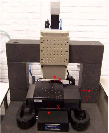
As it is possible to see from Fig. 5.27, it has been considered the force in the x direction. This represents the worst situation for the considered elements, because:

• about the Z- Stage: it is the case in which F has the biggest magnitude in a direction perpendicular to the z axis without any Y component of the force.;

• about the bridge: it has been seen from the theoretical analysis (see paragraph 5.3.2.1) that a cutting force in that direction is the worst situation, because it causes the biggest displacement of the bridge.

The Z-stage is assembled in a irreversible way with the bridge, so it is difficult to test the two elements separately. A way of action to test the bridge separately could be the following: apply a force to the bridge in the area close to the stage and measure the displacement in the same point. This method is not easy to apply, because:

Fig. 5.27-Bridge and Z-stage, with force and directions

• It would have been difficult to reproduce the same load configuration, in terms of force and moments, produced by the cutting force: in fact transferring the cutting force from the tool. To the bridge side (always in a x direction) it is necessary to add the moments in both the x and y directions;

• It would have been difficult to measure the displacement, for instance using a laser sensor, exactly in the same application point, because of the dimension of the bridge section (150mm X 150mm) that would have not allowed to interpolate the force’s value as for the tool.

For this motivations, it has been done some tests on both the elements together and it has been used the global value of the stiffness KBridge+Z-stage. To have an estimation of the stiffness of the

bridge and the Z-stage separately, theoretical and a FEM analysis of the bridge stiffness have been done.

5.3.2.1 Theoretical analysis

The aim of the theoretical analysis of the bridge is to have a qualitative behaviour of it, in order to have an estimation of its stiffness and a consequent value for the Z-stage stiffness.

The bridge has been modelled as a frame clamped at the machine base, as shown in Fig. 5.28. The characteristics of the section and of the bridge granite are shown in the Tab. 5.9.

Fx

X

Fig. 5.28-Bridge model and section.

where: side is the length of the side square section;

750 X 514 the dimension of the bridge.

Section Parameters side [mm] 150 A [mm2] 22,5*10^3 Ix [mm4] 42*10^6 I0 [mm4] 84*10^6 Granite Parameters E [MPa] 52.5*10^3 ν 0,25 G [MPa] 20*10^3

Tab. 5.9-section and granite parameters of the bridge

Due to the symmetry of the structure, it has been analyzed half a frame. This part is divided in two elements: QR and RS, as shown in Fig. 5.29.

In the theoretical analysis two possible situations have been taken into account (Fig. 5.30):

• Cutting force in X-direction;

• Cutting force in Y-direction. Considering the following hypothesis:

• Cutting force on the X-Y plane;

• The distance between the tool tip and the centre of gravity of the bridge is SP=315mm [Appendix E]. 514 750 Z Y X Z Y side

Fig. 5.29-Half-frame under exam mm p SP mm b RS mm l QR 315 375 514 = = = = = =

Where: P is the force application point.

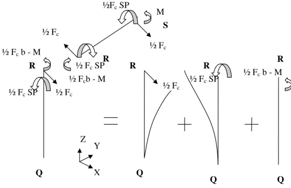
Fig. 5.30-Bridge model considered: cutting force in Y-direction (left), cutting force in X-direction (right)

On point S the cutting force Fc and the moment Fcp are acting. For the calculations only half the

force and half the moment are used because the other half acts on the other part of the bridge. Element RS can be modeled as a beam clamped at point S. Due to symmetry there is no angular displacement at point S. So there is a moment M in this point that brings the angular displacement to 0 (on the plane X-Y). The bending due to the force can be calculated with the “overlapping method”(Fig. 5.31). FCy FCx Z Y X Z Y X _R Q S Q R S

Fig. 5.31-Overlapping method applied to the bridge analysis

5.3.2.1.1 Cutting force in X-direction

The deflection

δ

θ

force Fc have been calculated as:

x c x c EI b F EI b F 6 3 ) 2 1 ( 3 3 1 = =

δ

Where: Fc is the cutting force; b is the distance RS;

Next θ2_{, rotation in the point S due to the moment M has been calculated as:}

x EI Mb = 2

θ

Where: M is the moment that causes the rotation θ2.

Because the rotation of point S on the plane X-Y is zero, θ1=θ2_{. Now the moment M can be}

calculated as: b F M EI Mb EI b F c c ⋅ = ⇒ = ⇒ = 4 1 2 ) 2 1 ( 2 2 1

θ

θ

Due to this moment follows the deflection δ2 _{at the point S as:}

EI b F EI b b F c c 8 2 ) 4 1 ( 2 3 2 = ⋅ =

δ

Now δ1_and δ2_{are known, so the total deflection in direction x of element RS can be}

determined as: EI b F EI b F EI b F_{c c c} totRS 24 8 6 3 3 3 2 1− = − = =

δ

δ

δ

Fig. 5.32-Load diagram of half a frame of the bridge

Since the milling is supposed to take place at a certain distance SP below point S, a moment of

Fcp is also acting on point S as shown in Fig. 5.31. This moment brings a twist in the element RS.

The twist has been calculated as:

o c RS GI b SP F ) 2 1 ( = Φ (5.23)

Where: G is the shear module;

Io is the polar moment of inertia.

Now the bending of element QR can be calculated. To do it, it is necessary to know which forces and moment are acting on point R, as shown in Fig. 5.32.

First the deflection and the rotation due to the cutting force have been calculated (plane X-Y) at the point R, as:

EI l F EI l F c c 6 3 ) 2 1 ( 3 3 3 = =

δ

Where:l is the distance QR.

EI l F EI l F c c 4 2 ) 2 1 ( 2 2 3 = = θ (5.25)

Then the deflection and rotation due to the moment generated by the cutting force (1/2 Fc SP)

have been calculated (plane X-Z) at the point R, as (SP=p):

EI pl F EI l p F c c 4 2 ) 2 1 ( 2 2 4 = = δ (5.26) EI pl F EI pl F c c 2 2 1 4 = = θ (5.27) ½ Fc b - M Q R S ½ Fc ½ Fc ½ Fc ½ Fc SP ½ Fc SP ½Fc SP ½ Fcb - M R Q R ½ Fc M Q R ½ Fc SP Q R ½ Fc b - M Z Y X

Fig. 5.33-Model with the force in Y-direction

Since these deflections and rotations act in the same plane those can be added:

EI p l l F EI pl F EI l F_{c c c} totQR 24 ) 6 4 ( 4 6 2 2 3 4 3 − = − = − =δ δ δ (5.28) EI p l l F EI pl F EI l F_{c c c} totQR 4 ) 2 ( 2 4 2 4 3 − = − = − =θ θ θ (5.29)

Now the twist generated by the moment caused by the cutting force and the distance b and the moment is calculated: o c o c c QR GI l b F GI l b F b F ) 4 1 ( ) 4 1 2 1 ( = − = Φ (5.30)

Now the deflections of element QR and RS are known, the total displacement and twist angle of point S can be calculated by “overlapping method”.

2 ₍1 ₎ 3 (4 6 ) ₄ 24 24 c c c Stot QR QR totRS o F b l F l l p F b b b EI GI EI

δ

δ

δ

Stot c th bridge F K δ = _ (5.33)

In order to compare that with the FEM analysis reported below, it is useful to evaluate the total deflection at the tool tip: it is the deflection of the bridge in point S together with the twist in point S times the arm SP times. The stiffness in this point is the total deflection divided by the cutting force.

o o Stot Stot c tip GI pb EI p l l EI b GI l b EI p l l p F K 2 4 ) 2 ( 24 4 24 ) 6 4 ( 1 3 2 2 ) ( + − − + + − = ⋅ Φ − =

δ

The obtained value is Kbridge_tip=84N/µm.

5.3.2.1.2 Cutting force in Y-direction

In the following paragraph the same calculations have been made with the force in the Y-direction (Fig. 5.33).

Due to symmetry it can not be any displacement in the Z- and Y-direction. So there will be a compressive force in element RS that is transferred to the QR element. Next to this there will be a

FCy

Z Y X

displacement due to the bending of element QR. At this moment it can already be concluded that the displacement of the point S in this configuration is smaller than the displacement in case of the cutting force in the other direction. So a calculation is not important in this direction, and it is possible to conclude the smaller stiffness of the bridge is the one obtained in the X-direction. For this motivation, the experimental tests and the FEM analysis have been done considering only the cutting force in the X-direction.

5.3.2.2 FEM analysis

In order to have an estimation of the qualitative behaviour of the bridge, it has been taken also the FEM analysis done previously by other authors.

All elements used for the bridge are 3D beam elements and the columns are clamped at the bottom (Fig. 5.34).

The material of the beams of the bridge is granite (Tab. 5.9).

Because there is a distance between the center of gravity of the spindle and the centre of the bridge, an element is inserted between node 13 and node 32. This element has no density and infinite stiffness. In front of the bridge is a column of 14 elements that simulates the spindle together with the Z-stage. The bending of the tool-tip and the bending of the stage + spindle are omitted in this analysis because no reliable information is available yet.

For the static analyses a force is applied at node 26. The force simulates the cutting force and the node simulates the tip of the milling tool in the model. Interesting for the accuracy is the displacement in this node caused by the cutting force. Axial forces are limited so only forces in the z- and x-direction are applied.

In Fig. 5.35 the deformed shape of the model is shown when a force of 20 N is applied in the z-direction.

The displacements are 0,0401µm in the y-direction (axial) and 0,0921µm in the z-direction.

In

Fig. 5.36 the same is shown for a force of 20 N in the x-direction.The displacement is 0,06 µm in the x-direction. From these results, the stiffness of the bridge relative to the tool-tip can be calculated.: Kbridge/tip/z =217 N/µm and Kbridge/tip/x = 333 N/µm.

Fig. 5.34-Bridge model

1 1 1 2 1 2 3 1 3 4 1 4 5 1 5 6 1 6 7 1 7 8 1 8 9 1 9 10 1 10 11 1 11 12 1 12 13 1 13 14 1 14 15 1 15 16 1 16 17 1 17 18 1 18 19 1 19 20 1 20 21 1 21 22 1 22 23 1 23 24 1 24 25 3 26 27 3 27 28 3 28 29 3 29 30 3 30 31 3 31 32 3 32 33 3 33 34 3 34 35 3 35 36 3 36 37 3 37 38 2 32 13 X Y Z studienr. Administrator DEC 1 2005 11:19:47 ELEMENTS MAT NUM

As it is possible to see (Fig. 5.35 and Fig. 5.36), the fem results are bigger than the theoretical (84 N/µm ). Anyway their meaning is to be a qualitative indication for the experimental test. So it is possible to conclude that, given that from the fem it is shown that the stiffness in x direction (y direction for the micro-milling machine reference system) is bigger than the one in the z-direction (x direction in the micro-milling machine reference system), the hypothesis done in the theoretical part are correct.

Fig. 5.35-Fem results for the bridge in Z-direction

Fig. 5.36-Fem results for the bridge in Y-direction

5.3.3 Experimental set-up

In order to evaluate the static stiffness of the Bridge+Z-stage is necessary to apply a force at the stage and measure the displacement as close as possible to the force application point. This latter should be representative of the position of the tool tip, where the cutting force is applied.

Looking to the construction drawing of the machine (Appendix A) it has been possible to find the distance between the inferior limit of the travel of the Z-stage and the tool-tip.

Therefore the aim of this paragraph is to find a way to apply the force to the Z-stage, at that point, and measure, at the same point, the displacement. The idea of applying the force on the inferior part of Z-stage is quite easy to employ, also because it is simple to place the instruments of the experimental set-up.

Considering that the Z-stage is directly assembled to the bridge, it is not necessary to have a clamping system for the target.

Concerning to the load, a device to apply the force is needed.

1 1 1 2 1 2 3 1 3 4 1 4 5 1 5 6 1 6 7 1 7 8 1 8 9 19 10 110 11 1 11 12 1 12 13 1 13 141 141511516116171711818119 1 19 20 1 20 21 1 21 22 1 22 23 1 23 24 1 24 25 3 26 27 3 27 28 3 28 29 3 29 30 3 30 31 3 31 32 3 32 33 3 33 34 3 34 35 3 35 36 3 36 37 3 37 38 2 32 13 X Y Z studienr. Administrator DEC 1 2005 11:22:29 DISPLACEMENT SUB =1 TIME=1 DMX =.101E-06 1 1 1 2 1 2 3 1 3 4 1 4 5 1 5 6 1 6 7 1 7 8 1 8 9 1 9 10 1 10 11 1 11 12 1 12 13 1 13 14 1 14 15 1 15 16 1 16 17 1 17 18 1 18 19 1 19 20 1 20 21 1 21 22 1 22 23 1 23 24 1 24 25 3 26 27 3 27 28 3 28 29 3 29 30 3 30 313 31 32 3 32 33 3 33 34 3 34 353 35 36 3 36 37 3 37 38 2 32 13 X Y Z studienr. Administrator DEC 1 2005 11:22:52 DISPLACEMENT SUB =1 TIME=1 DMX =.101E-06 1 1 1 2 1 2 3 1 3 4 1 4 5 1 5 6 1 6 7 1 7 88 1 99 1 10101 11 111 12 112 13 113 14 114 15 115 16 116 17171 18181 19 1 19 20 1 20 21 1 21 22 1 22 23 1 23 24 1 24 25 3 26 27 3 27 28 3 28 29 3 29 30 3 30 31 3 31 32 3 32 33 3 33 34 3 34 35 3 35 36 3 36 37 3 37 38 232 13 X Y Z studienr. Administrator DEC 1 2005 11:33:51 DISPLACEMENT STEP=1 SUB =100 TIME=1 DMX =.596E-07 1 1 1 2 1 2 3 1 3 4 1 4 5 1 5 6 1 6 7 1 7 8 1 8 9 1 9 10 1 10 11 1 11 12 1 12 13 1 13 14 1 14 15 1 15 16 1 16 17 1 17 18 1 18 19 1 19 20 1 20 21 1 21 22 1 22 23 1 23 24 1 24 25 3 26 27 3 27 28 3 28 29 3 29 30 3 30 31 3 31 32 3 32 33 3 33 34 3 34 35 3 35 36 3 36 37 3 37 38 2 32 13 X Y Z studienr. Administrator DEC 1 2005 11:33:30 DISPLACEMENT STEP=1 SUB =100 TIME=1 DMX =.596E-07

Due to the small load to apply (at most 25N) a wire with calibrated weights has been chosen, also because it is a very simple method to apply to that case with a planar surface as the Z-stage plate, with screw holes just done in the right position. The force applied on the Z-stage is then transfer to the bridge through the connection bridge-stage. As said before, it has been considered as a rigid connection, so it transfers all the loads to the bridge.

Finally it has been chosen the instrument to evaluate the displacement. From the literature it is known the expected value of the stiffness, so it is possible to calculate an estimated value of the displacement. It had been evaluated less then 10µm.

The Keyence laser has been chosen for measuring the displacement (see Chapter 3).

The experimental tests consisted on applying the force to the stage using calibrated weights up to 25N with a metallic wire of a 0,2mm diameter. To hung the weights, it has been used the same fixture used during the tool tests, fixed directly on the granite basement. To apply the load on the stage has been used a bolt screwed on the stage’s plate (Fig. 5.37). Several tests have been made with a two cycle loading for each. To measure the displacement closest as possible to the force application point, it has been used the laser sensor with a designed fixture, directly fixed on the Y-stage of the machine. This kind of set-up enables to move the sensor with the Y-stages control to find the right distance between it and the measured target. Before starting to collect the data, some test have been made to rely on the set-up and to check that it was stiff enough.

Fig. 5.38-Relative position wire-laser sensor

It has been possible to measure the displacement exactly under the application point, because of the thinness of the wire and the dimension of the elements under test (Fig. 5.38).

All the tests have been made with the machine system control operative. Therefore all the values found are compensated values. Anyway the Z-stage control acts only in the Z direction, so it does not influence the displacement in X-direction.

5.3.4 Experimental Results

The results of the bridge+Z-stage have been obtained applying a force from 0 to 24,5N. The displacement varied from 0µm to a range between 3,44~3,46µm. The behaviour of the chain bridge+Zstage is linear as shown in Fig. 5.39, and the trend line fitted to the experimental results shows an experimental static stiffness of Kexp_Bridge+Z-stage =7,09N/µm.

5.3.5 Conclusions and analysis of the results

Summarizing the results found with the theoretical, FEM and experimental analysis, as shown in the Tab. 5.10, it is possible to conclude that:

• the three values are really different from each other. Considering that the theoretical and the FEM analysis are just qualitative, and given the strong assumptions made to do them, it has been kept as considered as corrected the experimental value. In fact the hypothesis made during the theoretical and FEM analysis, such as an infinitive rigid connection, do not allow to reproduce the real case;

• Observing the qualitative results obtained with the theoretical and FEM analysis, and given that the value from the experimental test is much smaller than the others, it is possible to conclude that in the considered chain Bridge+Z-stage the latter is the most flexible element;

• In the literature [20] it has been found for the Z-stage a stiffness value of 1,73N/µm, so the experimental value obtained is not to be considered wrong.

Theoretical Bridge Stiffness [N/µm] 80 FEM Bridge Stiffness [N/µm] 190 Experimental Bridge+Z-stage Stiffness [N/µm] 7,09

Tab. 5.10-Bridge+Z-stage stiffness results

Fig. 5.39-Stiffness behaviour of bridge+Z-stage

Analysing possible error sources during the measurement, it is possible to find some factors that correct the experimental stiffness value. Starting from the experimental set-up, it is important to consider (see also Par.5.2.3.):

:

1. the stiffness of the sensor fixture: due to the very high sensibility of the laser sensor to every vibrations around its area (just walking around the sensor equipment gave a displacement on the sensor displayer), it has been necessary to have a very rigid fixture for it. It has been designed a small fixture, directly fasten on the Y-Stage, so it has been enabled the movement of it together with the stage. Thus it can be negligible the influence of the sensor fixture stiffness on the final value;

2. the alignment of the load application point and the pulley in a horizontal plane: the load application point on the stage is not perfectly aligned with the pulley in a horizontal plane. In fact to align them, it has been used the capacity of the operator: supposing that it is possible to appreciate by eyes at list 2°, it has been calculated that, the 99% of the real weight is transferred to the stage. So the corrective factor is falignment=0,99;

bridge+Zstage

fo

rc

e

[

N

]

3. the vibrations of the room: due the high sensibility of the laser sensor.. It has been observed on the display for the vibration amplitude of ±0,02µm. Given that the maximum displacement obtained was of 3,46µm, it means the 0,6% of the real displacement. It has increased the final value by 1%. So it is than possible to consider a corrective factor of fvibrations=0,99

The Tab. 5.11 shows the corrective factors found and the error budget of the experimental set-up:

Error Budget of the Experiemental Set-up Corrective factor Alignment pulley-application point 1% 0,99 Vibration's room 1% 0,99

Tab. 5.11-Error budget and corrective factors for the Bridge+Z-stage analysis.

Tt is possible to conclude that the correct value of the chain Bridge+Z-stage is Kcorr_Bridge+Z-stage

=6,95N/µm.

5.4

Spindle and tool-holder

5.4.1 Introduction

In order to evaluate the stiffness of the spindle, first of all it is necessary to consider the meaning of static stiffness for that component. The spindle mounted on the machine has a PID (see Chapter 3). When that is placed on a part, it has no sense to talk about “static stiffness”: in fact if a constant force is applied in a static condition when the control is active, it acts in order to bring the part back to the initial position, and it is not possible to see any displacement.

Looking at the literature, the value of the stiffness of the tool-holder depends on the type used in the machine. In fact depending on the kind of tool-holder and shank the stiffness value changes. In [13] is used a vertical conventional milling machine with a tool-holder REGO-0FIX ER8, which has a stiffness value of 1,4N/µm.

5.4.2 Design of method

Fig.5.40 shows the system that it is analyzed. As it is possible to see, it has been considered the force in the X-direction (red arrow in the Fig. 5.40). This represents the worst situation for the elements that have been considered (see paragraphs 5.3).

Evaluating the stiffness value of the tool-holder, it has to be kept in mind that the final value is due to the stiffness of all the elements involved in the considered chain shown in holder have been taken part to obtain the measured displacement.

Fig. 5.41 and analytically expressed by equation 5.34.

Knowing the values of the Bridge+Z-stage stiffness and the KT-Hchain value, it is possible to find

the stiffness of the chain spindle + tool-holder. With this last value, making some hypothesis on the behaviour of the spindle, it is easy to obtain the value of the tool-holder stiffness.

In order to evaluate the static stiffness of the tool-holder, three different analyses have been made: a theoretical one, a FEM one and an experimental one.

Fig. 5.40-Tool-holder, spindle, Z-stage, bridge Holder Tool Spindle Stage Z Bridge Hchain T K K K K ₋ = _{+ −} + + ₋ 1 1 1 1 (5.34)

Where: KT-Hchain is the equivalent stiffness of the chain. It is the value that it will be found with

this analysis;

Kcorr_Bridge+Z-stage is the stiffness value of the chain Bridge+Z-stage (see paragraph 5.2);

KSpindle is the stiffness of the spindle;

KTool-Holder is the stiffness of the tool-holder.

5.4.2.1 Theoretical analysis

Due to the fact that, as for the tool, it has been impossible apply the force at the same point where the displacement has been evaluated, it is necessary to use an interpolation factor to find the correct value of the stiffness: in order to find this interpolation factor is necessary to make some hypothesis on the behaviour of the chain spindle - tool-holder.

From the experimental analysis it has been evaluated a displacement at the end of the considered chain. In order to understand which elements were involved in that displacement, two different models have been considered, a “spindle + tool-holder compliance” model (Fig. 5.42) and a “tool-holder compliance” model (Fig. 5.45).

5.4.2.1.1 “Spindle + tool-holder compliance” model

The hypothesis of this model is that the displacement is due to both the compliance of the tool-holder and the compliance of the spindle. It means that both the spindle and the tool- tool-holder have been taken part to obtain the measured displacement.

Fig. 5.41-Tool-holder chain

Kcorr_BRIDGE

Fig. 5.42-“Spindle + tool-holder compliance” model

where: e is the distance between the two magnetic bearings;

f is the distance between the tool-holder tip and the front magnetic bearing; s is the axial coordinate along the spindle axis;

us is the displacement of the axis in a normal direction, function of the s coordinate.

δmax is the maximum displacement at the tool-holder tip due to the force F

F is the cutting force applied on the tool-holder tip

This model consider the spindle and the tool–holder as an isostatic beam, with a radial and axial constrains in the back bearing, and a radial constrain in the front one. The force is applied in a radial direction as said before.

To simplify the model, the spindle and the tool holder have been considered as a cylindrical beam, with a constant diameter Ds of the same material with an Young module E.

It is therefore possible to find the function us and the expression of the maximum displacement

δmax, using the Elastic Line Method.

x s s EI M s u = ∂ ∂ 2 2 (5.35) Where: Ms is the function of the moment due to the force F along the s coordinate.

    + ≤ ≤ − + ≤ ≤ = f e s e s f e F e s s e f F Ms ) ( 0 (5.36) Applying the boundary conditions, it can be obtained:

f e s e e s f e e e f es s f e s EI F s fe s e f EI F u x x s _{≤ ≤ +} ≤ ≤                    + +       + −       − +       − = 0 6 2 3 2 6 2 2 6 6 2 2 3 (5.37)

In order to use this analysis to correlate the experimental stiffness results, it has been necessary to evaluate the value of the interpolation factor α. To do that has been opportune to consider two different cases: the first one was an ideal case (Fig. 5.43), with the force applied to the tool-holder tip and the displacement measured at the same point; the second one was the real case (Fig. 5.44), with the force applied at the real application point, distant r from the tool-holder tip and the displacement measured under the tool-holder tip.

F e f s us δmax Ds Y X

Fig. 5.43-Ideal case in the tool-holder analysis

Fig. 5.44-Real case in tool-holder analysis

In order to link the two cases, it was necessary to equal the two maximum displacement δmax1

and δmax2, so to find the value of the force F1 that, applied on the tool-holder tip, gave a

displacement of the same magnitude of the one that has effectively been measured.

2 max 1 max δ δ = (5.38)

( )

(

)

(

)

( )

f e G r f e G F F − + = = α , , , 1 2 2 1 (5.41)

Where: F1 is the force applied on the tool-holder tip in the ideal case;

F2 is the force applied on a distance r from the tool-holder tip, in the real case;

G1 is a function of the geometrical parameters e and f;

G2 is a function of the geometrical parameters e, f and r.

IT has been possible at this point to calculate the stiffness value KTOOL as:

2 max 2 1 max 1 δ α δ holder Tool Spindle TOOL F F K = = + − (5.42)

and compare it with the theoretical value of the stiffness Kth=F1/δmax1 for this model.

5.4.2.1.2 “Tool-holder compliance” model

The hypothesis of this model has been that the displacement was due only to the compliance of the holder and the spindle is considered as infinitive rigid, so not to contribute to the tool-holder tip displacement. The model is represented in Fig. 5.45

This model considers the spindle as an infinitive rigid beam, linked in the front bearing with a finite rigid beam that represents the tool–holder. The latter has been modelled as a cylindrical beam with a diameter of DT-H and an Young module E. The force has been applied in a radial direction at

the tool-holder tip.

It has been therefore possible to find the function us that represented the displacement of the

tool-holder in a direction normal to the s coordinate along the spindle axis and the expression of the

maximum displacement δmax at the tool-holder tip, using the Elastic Line Method (equation 5.43).

F1 e f δmax1 F2 r δmax2