70
Chapter 5
THE HANDLING SURFACE
5.1. Introduction
The idea of a three dimensional graphic which represents how the vehicle’s directional behavior can be influenced by the tyre inflation pressure is here presented. It was already said that the handling diagram is unique for the vehicle and it depends on the constructive characteristics of it; moreover, considering a steady-state maneuver, the understeering gradient is only function of the steady-state lateral acceleration.
In the previous chapter the choice of set of tyres and inflation pressure has shown a sensible modification of the handling diagram. Because of this reason, the tyre inflation pressure can be considered as a new variable for the handling diagram. The understeering gradient is therefore influenced by this, and what is more important, the handling diagram is not longer unique. The steady-state directional behavior of the vehicle can be fully described by means of a surface; the understeering gradient is not anymore a scalar but can be replaced by the gradient of the surface.
What is important to remember is that the concept of handling surface was already presented by Dixon [1] and Frendo et al. [5]. However, in those publications the issue was addressed in different ways: in the first one, the effect of the vehicle longitudinal speed on the handling curve was shown. Moreover, the topic was not investigated in details; in the second one, the concept of handling surface was applied to vehicles fitted with locked differential. In this case the maneuver heavily affects the handling diagram, which therefore is no longer unique.
In this chapter the tyre inflation pressure will be considered the third variable of the handling diagram. It will be therefore represented as a surface. Different graphics for different set of tyres are shown.
71
5.2. Handling surfaces
The combinations shown in the Table 4-1 of the previous chapter are taken into account. Eight surfaces are plotted and discussed. Combination A and B are obtained with WRG2 set of tyres at front and rear; C and D are obtained with WRG2 set of tyres at front and RF at rear; E and F are obtained for RF at front and WRG2 at rear; G and H are obtained mounting RF at front and RF at rear.
In the pictures is reported a colorbar: it represents the understeering gradient K defined by equation (2.15). It is calculated in deg/g and its modification is reported in different colors (from blue color, representative of understeering behavior, to red color, representative of oversteering behavior).
5.2.1. WRG2 Front – WRG2 Rear
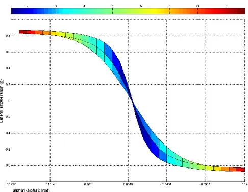
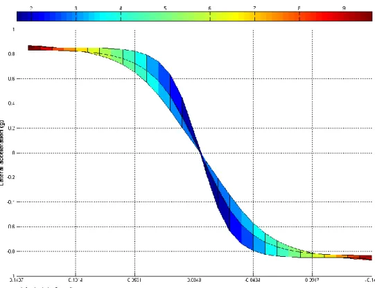
The surfaces for the Combination A and B are shown in three dimensions and on the / plane, respectively in Figure 5-1 and Figure 5-2 for Combination A, Figure 5-3 and Figure 5-4 for Combination B. The understeering gradient is reported in the colorbar.
72
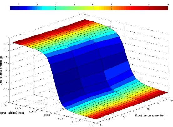
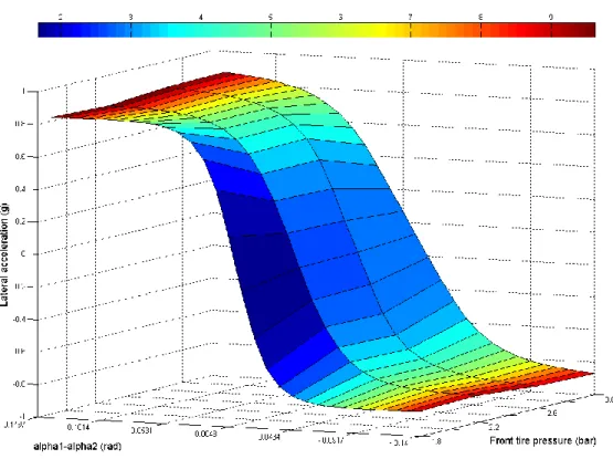
Figure 5-1 – Handling surface for Combination A: only the front tyre pressure changes
73
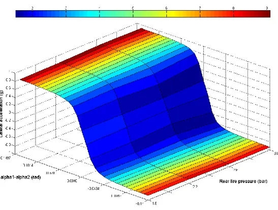
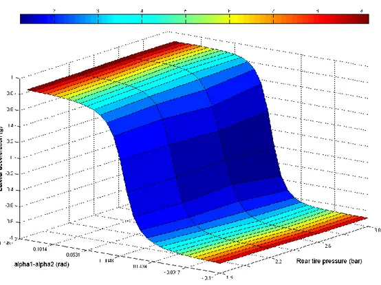
Figure 5-3 – Handling surface for Combination B: only the rear tyre pressure changes
74
There is only a slight modification of the diagrams in both cases (i.e. for lateral acceleration below 0.4 g, the understeering gradient becomes dark blue if the front pressure is increased; it becomes light blue if the rear pressure is increased); it is possible to say that for this set of tyres the influence of inflation pressure on the directional behavior of the vehicle is not so important.
5.2.2. WRG2 Front – RF Rear
The surfaces for the Combination C and D are shown in three dimensions and on the / plane, respectively in Figure 5-5 and Figure 5-6 for Combination C, and only in Figure 5.7 for Combination D. The reason why Combination D was represented in a different way is explained as follows: it was not possible to find in Matlab Cftool a function which could approximate the simulation data. For this reason, Excel was used.
75
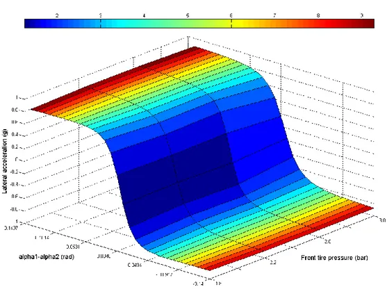
Figure 5-5 – Handling surface for Combination C: only the front tyre pressure changes
76
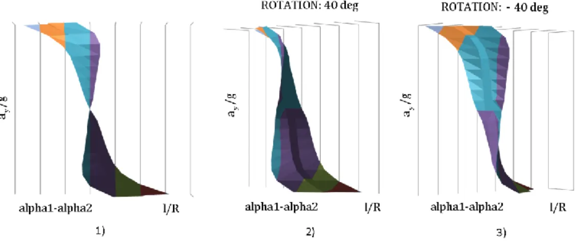
Figure 5-7 – Handling surface for Combination D, different views: 1) / plane; 2) Rotation of 40 deg on axis;
3) Rotation of -40 deg on axis
In this case there is a certain difference between the two combinations: modifying inflation pressure on front tyres only causes a slight modification of the handling diagram; on the contrary, increasing inflation pressure on the rear axle tyres causes an important modification of it: as it is possible to see from Figure 5-7 (but also from Figure 4-43,2), for pressure under 2.6 bar the vehicle is understeering; a pressure of 3.0 bar changes the vehicle directional behavior, which becomes oversteering. However, this phenomenon is reached only for a high inflation pressure that normally is not used in the tyres.
Moreover, combination D shows very clearly what happen to the vehicle modifying the inflation pressure of RF tyres. In fact, an important modification of the handling diagram is visible also for Combination E, G and H which are all cases of changing pressure at RF tyres.
5.2.3. RF Front – WRG2 Rear
The surfaces for the Combination E and F are shown in three dimensions and on the / plane, respectively in Figure 5-8 and Figure 5-9 for Combination E,
77
Figure 5-10 and Figure 5-11 for Combination F. The understeering gradient is reported in the colorbar.
Figure 5-8 – Handling surface for Combination E: ony the front tyre pressure changes
78
Figure 5-10 – Handling surface for Combination F: only the rear tyre pressure changes
79
Also here, as in the previous Combination C and D, it is possible to notice the difference between changing pressure on front axle (RF tyres, quite sensible modification of the handling diagram) and changing pressure on the rear axle (WRG2 tyres, slight modification of the handling diagram).
5.2.4. RF Front – RF Rear
The most extreme solution is here presented, respectively for Combination G and H. When a complete set of RF tyres for front and rear axle is used, it becomes very important the choice of tyres pressure: there are huge modifications of the directional behavior both for changing pressure on front axle tyres and rear axle tyres: in the first case, the result is similar to Combination E (the only difference between E and G is the tyres mounted at rear axle); in the second case the vehicle can have both understeering and oversteering behavior. All these considerations are better explained in pictures from Figure 5-12 to Figure 5-14.
80
Figure 5-13 – Handling surface for Combination G, / plane
Figure 5-14 – Handling surface for Combination H, different views: 1) / plane; 2) Rotation of 40 deg on axis;
81
5.2.5. Evaluation of the understeering gradient
The understeering gradient defined in 2.3 can be evaluated for a steady-state condition in the handling diagram. For example, the obtained considering a lateral acceleration of 0.4 g is taken into account. Most of the curves shown in the previous chapter are linear up to 0.4 g, so this point is considered. For the different combinations, the values of are evaluated in Table 5-1.
Combination Set K [deg/g] Combination Set K [deg/g] WRG2 1.8 – WRG2 1.8 A1 1.39 RF 1.8 – WRG2 1.8 E1 1.58 WRG2 2.2 – WRG2 1.8 A2 1.41 RF 2.2 – WRG2 1.8 E2 2.62 WRG2 2.6 – WRG2 1.8 A3 1.51 RF 2.6 – WRG2 1.8 E3 2.70 WRG2 3.0 – WRG2 1.8 A4 1.90 RF 3.0 – WRG2 1.8 E4 3.86 WRG2 1.8 – WRG2 1.8 B1 1.39 RF 1.8 – WRG2 1.8 F1 1.58 WRG2 1.8 – WRG2 2.2 B2 1.38 RF 1.8 – WRG2 2.2 F2 1.79 WRG2 1.8 – WRG2 2.6 B3 1.43 RF 1.8 – WRG2 2.6 F3 1.55 WRG2 1.8 – WRG2 3.0 B4 1.22 RF 1.8 – WRG2 3.0 F4 1.40 WRG2 1.8 – RF 1.8 C1 1.41 RF 1.8 – RF 1.8 G1 1.60 WRG2 2.2 – RF 1.8 C2 1.42 RF 2.2 – RF 1.8 G2 2.65 WRG2 2.6 – RF 1.8 C3 1.52 RF 2.6 – RF 1.8 G3 2.73 WRG2 3.0 – RF 1.8 C4 1.90 RF 3.0 – RF 1.8 G4 3.9 WRG2 1.8 – RF 1.8 D1 1.41 RF 1.8 – RF 1.8 H1 1.60 WRG2 1.8 – RF 2.2 D2 0.54 RF 1.8 – RF 2.2 H2 0.74 WRG2 1.8 – RF 2.6 D3 0.51 RF 1.8 – RF 2.6 H3 0.70 WRG2 1.8 – RF 3.0 D4 -0.53 RF 1.8 – RF 3.0 H4 -0.31
Table 5-1 – Evaluation of understeering gradient at = 0.4
From the previous table is possible to see which are the most understeering and oversteering conditions: with a set of RF front tyres at inflation pressure of 3.0 bar and a set of RF rear tyres at inflation pressure of 1.8 bar (Combination G4) the most understeering situation is reached. With a set of WRG2 front tyres at 1.8 bar and RF tyres at 3.0 bar the most oversteering condition is obtained.