INGEGNERIA DEI MATERIALI E DELLE STRUTTURE
XXI° CICLO
MODELLING THE LATERAL PEDESTRIAN FORCE
ON RIGID AND MOVING FLOORS BY A
SELF-SUSTAINED OSCILLATOR
Tesi presentata per il conseguimento del titolo
di Dottore di Ricerca in Ingegneria dei Materiali e delle Strutture
da
Andrea TROVATO
Coordinatore del Corso di Dottorato
Prof. Renato S. Olivito
Tutori del candidato
Prof. Domenico Bruno
Prof. Pierre Argoul
Università della CalabriaA Dio per avermi donato la forza e la salute
per raggiungere questo obiettivo.
Alla mia famiglia per l'amore sincero e
silenzioso con cui mi ha sostenuto.
DEPARTMENT OF STRUCTURES UNIVERSITY OF CALABRIA
Thesis for the Degree of Doctor of Engineering
Modelling the lateral pedestrian force on rigid and moving floors
by a self-sustained oscillator
by
Andrea TROVATO
ABSTRACT
For the serviceability analysis of civil engineering structures under human induced vibrations, a correct modelling of the pedestrian-structure interaction is needed. The proposed approach consists in thinking the human body as a Single Degree of Freedom oscillator: the force transmitted to the floor is the restoring force of this oscillator [1, 2]. In rigid floor conditions, such an oscillator must be able to reproduce two experimentally observed phenomena: (i) the time-history of lateral force can be approximated by a periodic signal with a “natural” frequency related with the single pedestrian characteristics; (ii) the motion of a pedestrian is self-sustained, in the sense that the pedestrian produces by itself the energy needed to walk.
Accounting for these aspects, a modified Van der Pol (MVdP) oscillator is proposed here to represent the lateral pedestrian force. The suitable form of its nonlinear restoring force is inferred from experimental data concerning a sample of twelve pedestrians. The experimental and model lateral forces show an excellent agreement.
For a laterally moving floor, the MVdP oscillator representing a pedestrian becomes non-autonomous. It is well-known that self-sustained oscillators in the non-autonomous regime are characterized by the so-called
Abstract
frequency switches from the ”natural” value to that of the external force: the response frequency is entrained by the excitation frequency. According to the physical interpretation considered here, the entrainment corresponds to the situation where the pedestrian changes its natural walking frequency and synchronizes with the floor oscillation frequency. The steady response of the MVdP oscillator subjected to a harmonic excitation is discussed in terms of non-dimensional amplitude response curves, obtained using the harmonic balance method truncated at the first harmonic. The model predictions are compared with some experimental results concerning pedestrians available in the literature and a good agreement is obtained. These topics are detailed in this thesis and also in the companion papers [3, 4] and in the report [5].
Keywords: pedestrian lateral force, self-sustained oscillator, modified Van der Pol
Index
Abstract ... i
List of symbols and abbreviations ... vii
List of Figures ... ix
List of Tables ... xiii
Chapter 1 Introduction ... 1
Chapter 2 Modelling the lateral pedestrian force on a rigid floor by a self-sustained oscillator ... 5
2.1. Introduction ... 6
2.2. The pedestrian as a single mass oscillator ... 7
2.3. The lateral force of a single pedestrian on rigid floor: experimental results ... 10
2.4. A modified Van Der Pol model for the lateral pedestrian force ... 20
2.4.1. Existence and stability of the periodic orbit ... 26
2.4.2. Energy analysis ... 28
2.5. Identification of the MVdP parameters from experimental data of the lateral pedestrian force ... 30
2.5.1 Procedure ... 30
2.5.2 Results ... 31
2.6. Conclusions ... 37
Chapter 3 A modified Van der Pol oscillator for modelling the lateral pedestrian force on a moving floor. Part I: response curves ... 39
Index
3.2. Models for the lateral pedestrian force ... 42
3.2.1. The Modified Van der Pol model ... 42
3.2.2. The model of Hof and coworkers ... 44
3.3. Modified Van der Pol model: harmonic balance and amplitude equation in the non-autonomous regime ... 46
3.3.1. Response curves - r²... 49
3.3.2. Analytical vs. numerical results ... 58
3.4. Force amplitude curves at constant frequency ... 59
3.4.1. Analytical vs. numerical results ... 62
3.4.2. Numerical vs. experimental results ... 65
3.5. Conclusions ... 66
Chapter 4 A modified Van der Pol oscillator for modelling the lateral pedestrian force on a moving floor. Part II: stability and synchronization ... 69
4.1. Introduction ... 70
4.2. Summary of the proposed model ... 71
4.2.1. Normalization, fixed points, amplitude equation ... 72
4.3. Local stability of the entrained steady response ... 74
4.3.1. Representation in the ν-r² plane ... 76
4.3.2. Representation in the ν- plane ... 79
4.4. The use of the stability domain for predicting the pedestrian synchronization ... 90
4.4.1. Analytical viewpoint: a 3D normalized synchronization domain ... 90
4.4.2. Analytical vs. numerical synchronization domain ... 92
4.4.3. Percentages of synchronization for a group of pedestrians ... 95
4.5. Conclusions ... 97
Chapter 5 Conclusions ... 99
Chapter 6 Appendix ... 101
B. Perturbation analysis of the MVdP model ... 102
C. Perturbation of the steady solution ... 104
D. The condition = ... 108
Index
List of Symbols and Abbreviations
BH Hopf Bifurcation
BN Node-Spiral Bifurcation
BS Saddle-Node Bifurcation
HB Harmonic Balance
FFT Fast Fourier Transform
SDoF Single Degree of Freedom
MVdP Modified Van der Pol
a=[a1, a2, a3, a4, a5]T vector of the parameters used for the identification f1 [Hz] fundamental frequency of the lateral pedestrian force h(uy, u ;y 0, , , ) nonlinear damping term
m [kg] mass of a single degree of freedom oscillator
p=[0, , , , ]T vector of the parameters of the modified Van der Pol model
r non-dimensional response amplitude
üabs [m/s2] absolute acceleration of m
u(t)=[ux(t),uy(t),uz(t)]T vector of the displacement of m
uy,per (t) [m] periodic approximation of the lateral pedestrian
displacement
vx [km/h] walking speed
Aacc [m/s2] floor acceleration amplitude
Ad [m] floor vibration amplitude
Ck [N] amplitude of the Fourier components of the lateral
List of Symbols and Abbreviations
C1,dyn [N] amplitude of the periodic lateral force applied on the floor
by a walker assuming entrained conditions
F=[Fx, Fy, Fz] [N] restoring force of a three degrees-of-freedom dynamic system
Fy,per (t) [N] periodic approximation of the lateral pedestrian force
T [s] period of the oscillator
S set of the admissible values for the parameters vector a
normalized form of the parameter
λ non-dimensional external acceleration amplitude
non-dimensional difference (detuning) between the floor frequency and the frequency 0 of the underlying linear
system associated with the MVdP oscillator
k [rad] phase of the k-th Fourier component [rad/s] frequency of the floor
0 [rad/s] circular frequency of the underlying linear system associated
with the MVdP oscillator
1 [rad/s] natural frequency of the autonomous MVdP oscillator
Δ1,k := k - k 1 [rad] phase difference of the k-th Fourier component
Δ[J] variation of on a period T [J] total mechanical energy
List of Figures
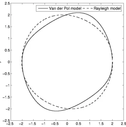
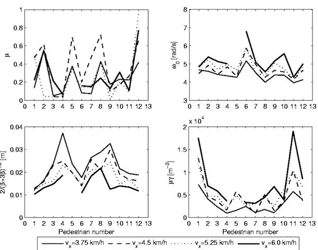
Figure 2.1 : Scheme of the SDoF system representing the lateral motion of a pedestrian. ... 8 Figure 2.2 : Pedestrian “8”: time-history of the lateral force for four different walking speeds. Experiment (continuous line) vs. Fourier Series (dashed line) according to Eq. (2.10). ... 11 Figure 2.3 : FFT modulus of the lateral walking force of pedestrian “8”. ... 13 Figure 2.4 : Frequencies and maximum displacement amplitudes for all pedestrians. Pedestrians are numbered according to the increasing mass order. Missing points correspond to non available experimental data. ... 16 Figure 2.5 : Fourier series amplitudes C1, C3 and phase differences Δ1,3 of the lateral force for all pedestrians. Missing points correspond to non available experimental data. ... 18 Figure 2.6 : Lateral oscillation of the pedestrian “8” (walking speed 4.5 km/h). Fourier series results. (a) Time history of pedestrian-induced lateral force; (b) time history of lateral displacement and (c) velocity; (d) modulus of the FFT of the lateral force; (e) limit cycle in the phase-plane and (f) lateral force as a function of displacement and velocity. ... 19 Figure 2.7 : Lateral oscillation of the pedestrian “8” (walking speed 6.0 km/h). Fourier series results. (a) Time history of pedestrian-induced lateral force; (b) time history of lateral displacement and (c) velocity; (d) modulus of the FFT of the lateral force; (e) limit cycle in the phase-plane and (f) lateral force as a function of displacement and velocity. ... 19 Figure 2.8 : Phase plots for all pedestrians. ... 20 Figure 2.9 : The different shapes of the limit cycles for the Van der Pol and Rayleigh's models: x u y, y u y/1, where 1 is the pulsation of the
autonomous oscillator. Parameter values: =0.15, 0=1 and =1 for the Van der Pol model; =0.1, 0=1 and =1/3 for the Rayleigh's model. ... 22
List of Figures
Figure 2.10 : Convention for the cartesian and polar coordinates in the phase plane. .. ... 24 Figure 2.11 : Lateral oscillation of pedestrian “8”; vx=4.5 km/h. Identified (dotted line) vs. Fourier series (continuous line) results. (a) Time history of the lateral force; (b) time history of lateral displacement and (c) velocity; (d) modulus of the FFT of the lateral force; (e) limit cycle in the phase-plane and (f) lateral force as a function of displacements and velocities. ... 32 Figure 2.12 : Lateral oscillation of pedestrian “8”; vx=6.0 km/h. Identified (dotted line) vs. Fourier series (continuous line) results. (a) Time history of the lateral force; (b) time history of lateral displacement and (c) velocity; (d) modulus of the FFT of the lateral force; (e) limit cycle in the phase-plane and (f) lateral force as a function of displacements and velocities. ... 33 Figure 2.13 : Identified MVdP model for pedestrian “8”. Time-evolution during a walking step of the energy terms associated with the nonlinear damping. The continuous thin line indicates the energy produced to sustain the oscillation. ... 34 Figure 2.14 : Identified parameters of the MVdP model for the twelve pedestrians. Missing points correspond to non available experimental data. 35 Figure 2.15 : Comparison between the Fourier series computed from experimental lateral force data (continuous line) and from the force associated with the identified MVdP models (dotted line). The comparison concerns the amplitudes C1 and C3 and phase differences Δ1,3. ... 36 Figure 2.16 : Correlation R between the lateral force computed by the Fourier series and the one associated with the identified MVdP model. ... 37 Figure 3.1 : (a) Scheme of the Two-Degrees-of-Freedom system representing the coupled lateral motion of a pedestrian and the deck of a footbridge. (b) Single-degree-of-freedom oscillator representing a pedestrian on a floor undergoing a harmonic motion. ... 44 Figure 3.2 : Response curves of the MVdP oscillator for the (a) isochronous case (=0) and (b) non-isochronous case (example with =2). The curves show the real and positive solutions of Eq. (3.18). Dotted line: =0.15, dashed line: =0.35, solid line: =1.0. ... 51
Figure 3.3 : Response curves of the MVdP oscillator (dotted lines) and conics associated with the condition (3.25) (solid lines). The other straight lines are related with the stability of the response. ... 53 Figure 3.4 : Plot of the polynomial p(z), Eq. (3.23), for = 1, = 1.4492 and five -values. ... 54 Figure 3.5 : Response curves of the MVdP oscillator (Eq. (3.18)) for = 1 and with five different -values. The vertical line corresponds to = 1.4492, while the dashed ellipse is associated with the condition (3.25). ... 54 Figure 3.6 : Response curves of the MVdP oscillator (Eq.(3.18)) for =1. Comparison between numerical and analytical results for three different -values. ... 58 Figure 3.7 : Pedestrian “2” - vx=3.75 km/h. Parametric plot of the amplitude of the lateral pedestrian force vs. the floor oscillation amplitude. The branch PQ is unstable. ... 62 Figure 3.8 : Pedestrian “2” - vx=3.75 km/h. Dynamic Load Factor vs. floor displacement amplitude at constant floor frequency: (a) 0.75 Hz and (b) 1.0 Hz. Comparison between analytical and experimental results. ... 63 Figure 3.9 : Pedestrian “1” - vx=3.75 km/h. Dynamic Load Factor vs. floor displacement amplitude at constant floor frequency: (a) 0.75 Hz and (b) 1.0 Hz. Comparison between analytical and experimental results. ... 64 Figure 3.10 : Dynamic Load Factor vs. floor displacement amplitude at constant floor frequency: (a) 0.75 Hz and (b) 1.0 Hz. Comparison between numerical results (pedestrians “1” and ”2”, vx=3.75 km/h) and experimental results (from the articles cited in the legend). ... 66 Figure 4.1 : Response curves and stability regions of the MVdP oscillator. Dotted lines: response amplitude curves associated with Eq. (4.14). Continuous lines: conic associated with the saddle-node bifurcation (4.21). Dashed-dotted lines: Hopf bifurcation (4.22). Dashed lines: nodes-spirals bifurcation (4.23)..77 Figure 4.2 : Bifurcations portraits of the MVdP oscillator in the parameter plane (, ). Case = 0. Global view and detail of the zone around the right cusp A of the saddle-node bifurcation BS. ... 82
List of Figures
Figure 4.3 : Bifurcations portraits of the MVdP oscillator in the parameter plane (, ). Case = 0.5. ... 83 Figure 4.4 : Bifurcations portraits of the MVdP oscillator in the parameter plane (, ). Case =1. Global view and (a) detail of the zone around the left cusp of BS; (b) detail of the zone inside BS where the branches of the node-spiral bifurcation BN intersect; (c) detail of the zone around the right cusp of BS. ... 84 Figure 4.5 : Bifurcations portraits of the MVdP oscillator in the parameter plane (, ). Case = 2. ... 85 Figure 4.6 : Surface representing the lower boundary of the stability domain, according to the analytical approximation defined in Table 4.5. Each point over the surface represents a pedestrian synchronized with the harmonically moving floor. ... 89 Figure 4.7 : Comparison between the analytical and numerical estimations of the boundary of the stability domain of the MVdP oscillator. Case = 0. ... 93 Figure 4.8 : Comparison between the analytical and numerical estimations of the boundary of the stability domain of the MVdP oscillator. Case = 0.5. ... 94 Figure 4.9 : Comparison between the analytical and numerical estimations of the boundary of the stability domain of the MVdP oscillator. Case = 1. ... 94 Figure 4.10 : Time-evolution of the displacements of the center of mass of pedestrian “2” (vx = 3.75 km/h) in the case of (a) non-entrained oscillation (Aacc = 0.05 m/s2, /(2)=1 Hz) and (b) entrained oscillation (Aacc = 0.15 m/s2, /(2)=1
Hz). uy : relative displacement; Uy + uy : absolute displacement; Uy : shake table displacement. ... 95
List of Tables
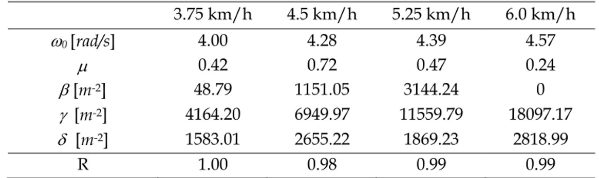
Table 2.1 : Mass and height of the twelve pedestrians involved in the tests performed at the Decathlon Research Center. ... 10 Table 2.2 : FFT of the lateral force of pedestrian “8”. Frequencies and amplitudes of the odd harmonics from order 1 to 9. ... 15 Table 2.3 : Pedestrian “8”, Fourier series analysis: amplitudes and phase differences of the odd harmonics from order 1 to 9, at different walking speeds. The fundamental frequencies are estimated by the FFT. ... 15 Table 2.4 : Average values on the set of twelve pedestrians of the walking frequency, the amplitudes and phase differences for the first five odd harmonics of the lateral force. ... 17 Table 2.5 : MVdP model: the identified parameters associated with pedestrian “8”. ... 32 Table 3.1 : Coordinates (z; ; ) of the points where the conic (3.25) has vertical tangent. ... 57 Table 4.1 : Coordinates (z; ; ) of the points O and O’, at the intersection of BS,
BH and BN. ... 78 Table 4.2 : Coordinates z and (, ) of the cusp points of the saddle-node bifurcation BS. ... 85 Table 4.3 : Description of the fixed points in the different regions of the bifurcation diagrams. First part. (s.n.=stable node; s.s.= stable spiral; sd.= saddle; u.n.= unstable node; u.s.=unstable spiral). ... 87 Table 4.4 : Description of the fixed points in the different regions of the bifurcation diagrams. Second part. (s.n.=stable node; s.s.= stable spiral; sd.= saddle; u.n.= unstable node; u.s.=unstable spiral). ... 87 Table 4.5 : Inequalities defining the stability domain for the entrained solutions (4.5)-(4.10) of the non-utonomous MVdP oscillator (4.4), according to the analytical approximation based on the harmonic balance method. Q = Q (, ) and H = H (, ) are defined by Eqs. (4.25) and (4.26), respectively. .... 88
List of Tables
Table 4.6 : Percentages of synchronized pedestrians in a population of twelve people. The average of the natural walking frequencies of all pedestrians is f1
= 0.848 Hz with a standard deviation of 0.055 Hz. ... 96 Table 4.7 : Percentages of synchronized pedestrians in a population of twelve people. The average of the natural walking frequencies of all pedestrians is f1
= 0.923 Hz with a standard deviation of 0.053 Hz. ... 97
Chapter 1
Introduction
The increased use of large span floors within buildings and of light and streamlined footbridges around the world as well as the increasing number of full-crowded stadium during concerts or matches have emphasized the incidence of human induced vibration problems in the design of civil engineering structures. Famous examples of such phenomena can be found in newspapers and in scientific literature. One was during the 1985 Bruce Springsteen concert in the Ullevi Stadium of Göteborg (Sweden), where the rhythmic movement (vertical jumping) of tens of thousands of people was close to causing a structural collapse. Another was during the opening day of the Millennium Footbridge in London, where due to people crossing, the south span had been moving laterally through an amplitude of about 50 mm at 0.8
Hz and the center span about 75 mm at 1 Hz approximately. In both cases, the
stadium and the footbridge were closed to public for two years in order to remedy these vibration problems.
Other situations, similar to the Millennium Footbridge with unexpected large lateral vibrations, occurred in 1999 on the Solférino footbridge in Paris [6] and, more recently, the same behavior has been detected on the “Pedro and Ines footbridge” in Coimbra, Portugal, during the tests carried out before the opening of the structure [7].
Most of problems are caused by feet impacts which generate a nearly periodic force with a frequency close to the natural frequency of the floor or the structure in contact with feet: a resonance phenomenon is activated. In the case of footbridges, when the first mode of lateral vibration falls in the same frequency range of the pedestrians' walking frequency (this was the case for the Millennium Footbridge in London and the Solférino Footbridge in Paris), the amplitude of the structural oscillations increases and pedestrians are forced to change their way of walking when the oscillation amplitude is large
Introduction
enough. A certain percentage of pedestrians changes the walking frequency, synchronizing the rhythm of the walk with that of the bridge deck oscillation. This phenomenon of structure-pedestrian synchronization has been often experimentally detected and has been analyzed in several studies [6, 8-14]. Recently, [15] proposed a model for the evaluation of the crowd lateral force accounting for the “saturation” phenomenon, i.e. the fact that the synchronization cannot occur when the footbridge oscillation amplitude becomes too large, since pedestrians stop walking; see also [13].
In order to correctly model the pedestrian-structure interaction, a good understanding of the pedestrian walking phenomenon is needed. The first phase of analysis should concern the basic case of a pedestrian walking on a
rigid floor: an extensive review of the scientific literature concerning this
situation is reported in [16]. The main information that can be extracted from the literature is that the walking force on a rigid floor is nearly periodic [17- 19]. Hence, the lateral (and vertical and longitudinal) component of the force exerted by a pedestrian on the floor can be represented by their Fourier series [16, 20]. In this thesis, it is often pointed out that the amplitude of the first superharmonics is not negligible in comparison with that of the fundamental component. The experimental analysis discussed here confirms this experimental finding. Moreover, a suitable definition of phase difference between the fundamental harmonic and each superharmonic is given, in order to clarify the experimental data interpretation. It is also proposed a “physical” interpretation for the first of the these phase differences, between the fundamental harmonic and the third superharmonics.
The human body is a complex dynamic system. Several more or less complicated approaches can be used to model such a system for rigid floor conditions; see for instance [21, 22]. Since our objective is the modelling of the lateral walking force component, a simpler approach is discussed here: the human body is thought as a Single Degree of Freedom (SDoF) dynamic system fulfilling some fundamental requirements observed from experimental results: (i) its mass is equal to the pedestrian mass; (ii) the time-history of lateral force is an approximately periodic signal with a fundamental frequency close to 0.8-1 Hz; (iii) the amplitude of the first five odd superharmonics is not negligible. The presence of superharmonics indicates that the SDoF oscillator must be nonlinear; (iv) the motion of pedestrians is “self-sustained”, i.e. he produces the energy needed to sustain its walk.
A modified Van der Pol (MVdP) model fulfils all previous requirements: like the standard Van der Pol (VdP) model, it is nonlinear and self-sustained, i.e. it possesses a stable limit cycle [23]. The suitable form of the model, i.e. the number and maximum power of the polynomial terms constituting the restoring force, is discussed in [1] and presented here. Moreover, the model parameters are identified from experimental data concerning a sample of twelve pedestrians walking on a rigid floor. Numerical and experimental results are discussed and compared.
According to this approach, the motion of the floor introduces an external excitation on the self-sustained oscillator representing the walker, that becomes non-autonomous. The last part of this thesis concerns the analysis of this situation. One of the most important properties of non-autonomous self-sustained oscillators is that they may have an entrained response [24], i.e. a response characterized by the same frequency as that of the excitation. The
entrained response of the MVdP model has never been analyzed, even if
analogous results are well-known for the standard Van der Pol model and for the Rayleigh model [23, 25]. Actually, an entrained response represents a pedestrian synchronized with the moving floor, even if its natural frequency is different. This interpretation explains the practical interest of the research of an
approximated analytical solution of the MVdP oscillator in the non-autonomous regime. The particular case of a harmonic excitation is considered, because a
floor lateral motion at constant frequency and amplitude is a simple experimental condition, easy to obtain using a shake table where pedestrians are asked to walk. This experimental situation is studied e.g. in [26]. A similar situation is obtained when pedestrians walk on a treadmill placed on a shake table [27, 28]. In addition, an harmonic excitation is the natural assumption required to apply the harmonic balance method.
After the Introduction, in Chapter II the general equation of motion of a SDoF oscillator schematically representing a pedestrian is given. Then, the main results of the experimental analysis performed on a set of twelve pedestrians on a rigid floor are presented. These outcomes are used to define the suitable restoring force of a self-sustained SDoF model able to reproduce the experiments. The parameters of this model are then identified and model predictions are finally compared with experimental results. Chapter III deals with the analysis of the moving floor case. The response amplitude equation for the MVdP oscillator is derived using the harmonic balance method. Then, the response curves at constant excitation frequency are compared with some
Introduction
experimental results concerning pedestrians walking on a shake table. Chapter IV recall the main relationships defining the amplitude of its stationary entrained response to a harmonic excitation. The main theoretical goal of this Chapter is the stability analysis of these responses. Then, the pedestrian-floor
Chapter 2
Modelling the lateral pedestrian force on a rigid
floor by a self-sustained oscillator
For the serviceability analysis of civil engineering structures under human induced vibrations, a correct modelling of the pedestrian-structure interaction is needed. The first phase of this modelling must concern the force applied by a pedestrian walking on a rigid floor: the present Chapter deals with the lateral component of this force. The approach proposed here consists in thinking the human body as a Single Degree of Freedom oscillator: the force transmitted to the floor is the restoring force of this oscillator. Such an oscillator must be able to reproduce two experimentally observed phenomena: (i) the time-history of lateral force can be approximated by a periodic signal and the amplitude of the first five odd superharmonics is not negligible; (ii) the motion of a pedestrian is self-sustained, in the sense that the pedestrian produces by itself the energy needed to walk. Taking into account these aspects, a modified Van der Pol (self-sustained) oscillator is proposed here to represent the lateral pedestrian force. A suitable form of its nonlinear restoring force is inferred from experimental data concerning a sample of twelve pedestrians. The experimental and model lateral forces show a good agreement.
Modelling the lateral pedestrian force on a rigid floor by a self-sustained oscillator.
2.1. Introduction
Several recently built footbridges have shown to be sensitive to the human induced vibration, e.g. the Millennium Footbridge in London, the Solférino Footbridge and the Simone de Beauvoir Footbridge in Paris. The causes of this phenomenon may be described as follows: the crowd walking on a footbridge imposes to the structure a dynamic lateral excitation at a frequency close to 1
Hz.When the first mode of lateral vibration of the footbridge falls in the same frequency range, a resonance phenomenon is activated. Hence, the oscillation amplitude increases and, provided that the oscillation amplitude becomes large enough, pedestrians change their way of walking, synchronizing their frequency with that of the bridge deck. This synchronization phenomenon has been often experimentally detected and has been analyzed in several studies, e.g. [6, 8 - 16].
In order to correctly model the pedestrian-structure interaction, a good understanding of the pedestrian walking mechanisms is needed. The first phase of this analysis must concern the basic case of a pedestrian walking on a rigid floor. The main information that can be extracted from the literature is that the walking force on a rigid floor is nearly periodic [17- 19]. Hence, the vertical, lateral and longitudinal components of the force exerted by a pedestrian on the floor can be represented by their Fourier series [16, 20]. In this thesis, it is often pointed out that the amplitude of the first harmonics is not negligible in front of that of the fundamental component. However, most of these experimental studies underestimate the importance of the phase information. This aspect will be discussed in this Chapter.
The human body is a complex dynamic system, but the modelling of the
lateral force exchanged by the feet with the floor could be based, as a first trial,
on the use of a single degree of freedom (SDoF) oscillator. Such an oscillator should be able to reproduce two experimentally observed phenomena: (i) the lateral force is quasi-periodic, with fundamental frequency close to one Hertz and where the first 4-5 odd super-harmonics are not negligible. This implies that the SDoF oscillator must be nonlinear; (ii) the motion of a pedestrian is “self-sustained”, in the sense that the pedestrian behaves like a system producing by itself the energy needed to walk. In order to represent these properties of the pedestrian lateral force, we propose here the use of a modified Van der Pol (VdP) model: like the standard VdP model, it is
nonlinear and self-sustained, i.e. it possesses a stable limit cycle in the phase plane [23].
After the Introduction, the general equation of motion of a SDoF oscillator schematically representing a pedestrian is given. Then, in Section 2.3, the main results of the experimental analysis performed on a set of twelve pedestrians are presented. These outcomes are used in Section 2.4 to define the suitable restoring force of a self-sustained SDoF model able to reproduce the experiments. The parameters of this model are identified according to a procedure discussed in Subsection 2.5.1 and results are presented in Subsection 2.5.2.
2.2. The pedestrian as a single mass oscillator
A pedestrian is a complex system composed of several interacting parts. To precisely model its behaviour under different "working" conditions, i.e. walking, running, bouncing, horizontal body swaying, etc., is a challenging task. As already said in the introduction, an interesting approach is based on the multi-body dynamics [21, 22], where each main part of the human body is represented by a rigid body connected with the other parts. In view of the stability analysis of a footbridge under the crowd load, simpler approaches have been used in several past studies [29-31]. In most of them, the single pedestrian is modeled as a discrete mass m subjected to the inertial forces and to the force of interaction with the bridge floor. The same approach based on a SDoF system representing a pedestrian is used here; see Fig. 2.1.
Modelling the lateral pedestrian force on a rigid floor by a self-sustained oscillator.
Figure 2.1: Scheme of the SDoF system representing the lateral motion of a pedestrian.
The equilibrium in an inertial reference of all the forces acting on m reads
absmu t F t mg (2.1)
where the superposed dot indicates the (partial) time-differentiation; m is the pedestrian mass; F=[Fx, Fy, Fz] is the contact force between the pedestrian and the bridge deck; g is the gravity acceleration vector; üabs(t) is the absolute acceleration of the mass m, accounting for both the motion of the floor and the relative acceleration ü(t) between m and the floor. The expression of üabs(t) in the general case is complex, since it depends on both the deck movement U(x,t), with x=[x, y, z]T the generic Lagrangian co-ordinate of a deck point, and the pedestrian motion, composed by its trajectory on the bridge floor and by the oscillations u(t)=[ux(t), uy(t), uz(t)]T relative to the floor. However, we consider here the case of a rigid horizontal floor and constant walking speed on a straight trajectory. Under these assumptions, one has üabs(t)=ü(t). Moreover, only the lateral oscillations of m are analyzed in this thesis: supposing that the x-axis is parallel to the straight trajectory, the lateral direction is parallel to the y-axis. Projecting (2.1) in this direction, one has
y y 0
mu t F t (2.2)
This relationship shows that when Fy(t) is known from measurements, the
motion uy(t) of the mass m can be derived. The next Section will concern this
analysis of experimental data collected from tests on a sample of twelve pedestrians walking on a rigid floor. A model for the force F can be defined as follows:
,
F F u u (2.3)
i.e. F is thought as the restoring force of a three degrees-of-freedom dynamic system, and it depends on the displacements and velocities relative to the floor. Projecting (2.3) in the y-direction under the same simplifying assumptions discussed above, one has
y y x, , , , ,y z x y z
F F u u u u u u (2.4)
where Fy depends on all the x, y, and z components of the displacements and velocities around the mean trajectory. Hence, this general expression accounts for a coupling between the different components. However, it is supposed here that this coupling is negligible, i.e.
y y y, y
F F u u
This leads to a single degree-of-freedom oscillator defined by the following dynamics equation (see also Fig. 2.1):
y y y ,y 0
mu t F u t u t (2.5)
In order to have a self-sustained oscillator, Fy must have some special characteristics, i.e. the solution uy(t) of the autonomous system (2.5) must have a stable periodic orbit in the phase plane [23]. A classical example of this kind of behaviour is given by the Van der Pol oscillator
Modelling the lateral pedestrian force on a rigid floor by a self-sustained oscillator.
y 0 2 2 0 0 , ; , , 2 1 y y y y y F u u u u u m (2.6)where 0 is the circular frequency of the underlying linear system, >0 and >0 are associated with the nonlinear damping term. The data analysis of Section 2.3 will show that the classical VdP model (2.6) is not general enough for well representing the walker lateral behaviour. For this reason a different self-sustained model is proposed in Section 2.4 and its parameters are identified in Section 2.5.
2.3. The lateral force of a single pedestrian on rigid floor:
experimental results
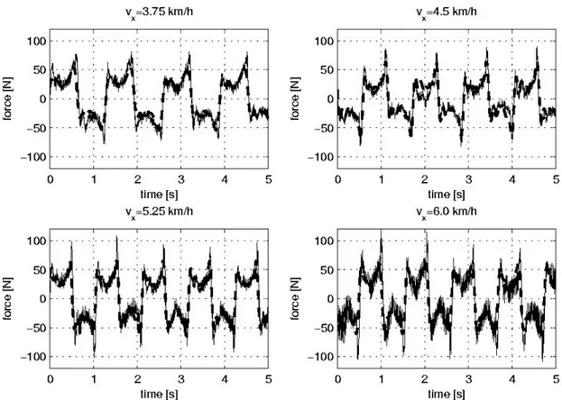
This Section is dedicated to the analysis of the experimental data provided by the Research Center of Decathlon in Villeneuve d'Ascq (France) concerning twelve pedestrians. The mass of pedestrians varies from 64 kg to 96 kg; see Table 2.1. They are numbered according to the increasing mass order. The lateral force of each walker has been measured at four different walking speeds: vx=3.75 km/h, vx=4.5 km/h, vx=5.25 km/h, vx=6.0 km/h. All walking conditions were realized on a treadmill dynamometer equipped with four force transducers, allowing to determine the ground reaction forces exerted under each foot [32].
Pedestrian 1 2 3 4 5 6 7 8 9 10 11 12
m (kg) 64 66 68 68 71 71 71 73 74 74 78 96
H (cm) 175 174 163 177 189 178 186 185 186 183 180 179
Table 2.1 – Mass and height of the twelve pedestrians involved in the tests performed at the Decathlon Research Center.
The nominal walking speed vx associated with each measure is the velocity of the treadmill during the test. The sampling time step is Δt=0.005 s, while the number of recorded force values is N=6000, corresponding to a signal length
tN=(N-1)Δt=29.995 s. The sets of the discrete instants and frequencies are then defined as {t}n=tn=(n-1)Δt and {f}m=fm=(m-1)Δf, respectively. The frequency increment is Δf=1/(N Δt)=0.0333 Hz. The recorded signals for pedestrian "8" at four different walking speeds are reported in Fig. 2.2. Hereafter, the main results will be illustrated with reference to the pedestrian "8". For all the other pedestrians, only a summary of the main results is given. For the complete data analysis, the reader is referred to [33].
Figure 2.2: Pedestrian “8”: time-history of the lateral force for four different walking speeds. Experiment (continuous line) vs. Fourier Series (dashed line) according to Eq.(2.10).
When a pedestrian walks on a rigid floor, along a straight trajectory and with constant speed, the force Fy(t) exerted on the floor is approximately periodic. This statement has been discussed by several investigators, e.g. [17-18]. Under this assumption, the measured force signal Fy(t) can be approximated by its Fourier series (see the Appendix A):
Modelling the lateral pedestrian force on a rigid floor by a self-sustained oscillator.
0 , 1 1 cos 2 2 y y per k k k C F t F t C kf t (2.7)where f1 is the pacing or fundamental walking lateral frequency; Ck>0 and k (-,] are the harmonic amplitudes and phases, respectively. Note that for a given periodic signal, the phases k depend on the initial time. Hence, their values are not physically significant. However, it is always possible to define a suitable translation of the time scale such that t t t= - 0 with 2f1t0-1=0. In this situation, one can write
0 , , 0 1 1, 1 : cos 2 2 y per y per k k k C F t F t t C kf t (2.8)with the phase “differences” defined as follows
Δ1,k:= k - k 1, for k ≥ 1
These quantities are an intrinsic property of a periodic signal. Hereafter, the tilde associated with the translated time-scale will be omitted for the sake of simplicity.
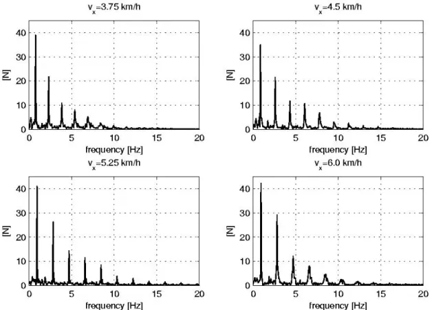
The recorded signals have been first analyzed by the Fast Fourier Transform (FFT), in order to find the fundamental frequency and to have an estimation of the relative amplitude between the different harmonics. The definition used here for the FFT reads
2 1 1 1 2 ˆ N i m n N y y n F m F n e N for m=1,…,N (2.9)where N t is the length of the largest time-interval of the recorded signal containing an integer number of periods. According to (2.9),
ˆ : ˆ 1
y m y
F f F m . The factor 2 /N introduced in (2.9) leads to define a complex quantity Fˆy, measured in Newtons, whose modulus is directly comparable to the Fourier series coefficients Ck. The plots of the modulus of Fˆy for the lateral walking force of pedestrian “8” at several walking speeds are given in Fig. 2.3. The Nyquist frequency is equal to fNy=1/(2Δt)=100 Hz, but, for the sake of clarity, the plot is represented up to f=20 Hz. As a matter of fact,
this analysis shows that the first odd harmonics up to that of order 9 are non negligible for all walking speeds. This confirms analogous findings of other authors, e.g. [20]. More in detail, for the pedestrian “8”, the peaks having amplitude greater than 3-4 N are those of the harmonics of order 1, 3, 5, 7, 9. The harmonics 11 and 13 and the even harmonics always have smaller amplitude. The mean value of the walking force Fy, estimated from
ˆ 1 /2
y
F m is also small in general. Similar results have been found for the other eleven pedestrians.
Figure 2.3: FFT modulus of the lateral walking force of pedestrian “8”.
In summary of this study, it is assumed that the lateral force can be approximated as a periodic signal with zero mean limited to its odd harmonics from the order 1 to 9:
max , 2 1 1 1,2 1 1 cos 2 2 1 k y per k k k F t C k f t (2.10)Modelling the lateral pedestrian force on a rigid floor by a self-sustained oscillator.
with kmax=5. Assuming that Eq. (2.2) holds, one has an estimation of the experimental acceleration of m by the following expression
, max , 2 1 1 1,2 1 1 1 cos 2 2 1 k y per y per k k k F t u t C k f t m m (2.11)from which the analytical expressions of the lateral velocity and displacement can be easily found:
max max 2 1 , 1 1,2 1 1 1 2 1 , 2 1 1,2 1 1 1 1 sin 2 2 1 2 2 1 1 cos 2 2 1 2 2 1 k k y per k k k k y per k k C u t k f t m k f C u t k f t m k f (2.12)The frequencies and amplitudes of the first odd harmonics computed using (2.9) are collected in Table 2.2. The fundamental frequency estimation obtained from the FFT is retained, while the amplitudes C2k-1 and phase differences Δ1,2k-1 are computed by a Fourier series analysis. The results of Table 2.3 are obtained. The frequencies and amplitudes are similar to those computed by the FFT. The measured force and the periodic approximation are compared in Fig. 2.2.
3.75 km/h 4.5 km/h 5.25 km/h 6.0 km/h f1 [Hz] 0.77 0.87 0.941 0.943 f3 [Hz] 2.31 2.61 2.82 2.83 f5 [Hz] 3.85 4.34 4.70 4.72 f7 [Hz] 5.39 6.08 6.59 6.60 f9 [Hz] 6.93 7.82 8.47 8.56
1
ˆ y F f N 38.96 34.88 41.01 42.26
3
ˆ y F f N 21.75 21.45 26.26 29.17
5
ˆ y F f N 10.74 11.7 14.28 11.99
7
ˆ y F f N 8.00 10.54 11.47 7.97
9
ˆ y F f N 5.25 6.85 8.40 4.55Table 2.2 – FFT of the lateral force of pedestrian “8”. Frequencies and amplitudes of the odd harmonics from order 1 to 9.
3.75 km/h 4.5 km/h 5.25 km/h 6.0 km/h f1 [Hz] 0.77 0.87 0.941 0.943 C1 [N] 39.10 34.91 41.08 42.28 C3 [N] 21.16 21.59 26.19 29.37 C5 [N] 9.25 11.73 13.70 12.26 C7 [N] 5.76 10.79 10.69 8.32 C9 [N] 3.04 7.38 7.17 3.68 Δ1,3 [rad] 2.47 2.42 2.92 2.66 Δ1,5 [rad] -1.48 -1.56 -0.52 -0.66 Δ1,7 [rad] 1.12 0.92 2.28 2.19 Δ1,9 [rad] -1.87 -2.71 -0.98 -0.97
Table 2.3 – Pedestrian “8”, Fourier series analysis: amplitudes and phase differences of the odd harmonics from order 1 to 9, at different walking speeds. The fundamental frequencies are estimated by the FFT.
Modelling the lateral pedestrian force on a rigid floor by a self-sustained oscillator.
Figure 2.4: Frequencies and maximum displacement amplitudes for all pedestrians. Pedestrians are numbered according to the increasing mass order. Missing points correspond to non available experimental data.
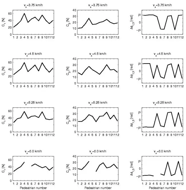
Fig. 2.4 shows the fundamental walking frequencies and the lateral displacement amplitudes for all pedestrians. The values of the amplitudes C1 and C3 and of the phase differences Δ1,3 are depicted in Fig. 2.5. Table 2.4 collects the corresponding averages.
3.75 km/h 4.5 km/h 5.25 km/h 6.0 km/h f1 [Hz] 0.848 0.919 0.975 1.033 C1 [N] 40.29 41.20 41.79 39.33 C3 [N] 17.37 19.11 22.06 21.41 C5 [N] 6.38 6.55 9.45 8.64 C7 [N] 3.51 2.79 5.15 5.26 C9 [N] 2.36 1.43 2.78 2.23 Δ1,3 [rad] -2.91 -3.04 3.10 2.92 Δ1,5 [rad] 0.41 0.34 -0.08 -0.45 Δ1,7 [rad] -2.62 -2.39 3.10 2.77 Δ1,9 [rad] 0.71 1.23 -0.02 -0.31
Table 2.4 – Average values on the set of twelve pedestrians of the walking frequency, the amplitudes and phase differences for the first five odd harmonics of the lateral force.
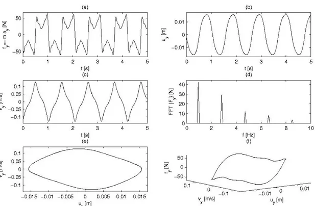
The displacement amplitudes of Fig. 2.4, as well as the displacement and velocity curves of Figs. 2.6 and 2.7 are computed using (2.10), (2.11) and (2.12). The displacement amplitude is about 1.8 cm, while the velocity amplitude is about 0.15 m/s. These values are very close to those measured by other authors; e.g. [34]. Moreover, observe that periodic orbits in the phase plots of Figs. 2.6e and 2.7e are characterized by a maximum velocity amplitude in the second and fourth quadrant. The phase plots are also depicted for all pedestrians and all walking speeds (Fig. 2.8): at a given speed, the orbit shape can change from one pedestrian to the other. These variations can be mainly attributed to the value of Δ1,3, as it is explained in the next Section. One can also notice that for increasing walking speeds, the amplitude of the lateral displacement and velocity decreases: a greater walking speed is accompanied by a smaller lateral oscillation. The measurements of [34] confirm this result. The three-dimensional plots in Figs. 2.6f and 2.7f show the lateral force as a function of displacements and velocity using the harmonics up to 9th order.
Modelling the lateral pedestrian force on a rigid floor by a self-sustained oscillator.
Figure 2.5: Fourier series amplitudes C1, C3 and phase differences Δ1,3 of the lateral force for
Figure 2.6: Lateral oscillation of the pedestrian “8” (walking speed 4.5 km/h). Fourier series results. (a) Time history of pedestrian-induced lateral force; (b) time history of lateral displacement and (c) velocity; (d) modulus of the FFT of the lateral force; (e) limit cycle in the phase-plane and (f) lateral force as a function of displacement and velocity.
Figure 2.7: Lateral oscillation of the pedestrian “8” (walking speed 6.0 km/h). Fourier series results. (a) Time history of pedestrian-induced lateral force; (b) time history of lateral displacement and (c) velocity; (d) modulus of the FFT of the lateral force; (e) limit cycle in the phase-plane and (f) lateral force as a function of displacement and velocity.
Modelling the lateral pedestrian force on a rigid floor by a self-sustained oscillator.
Figure 2.8: Phase plots for all pedestrians.
2.4. A modified Van Der Pol model for the lateral pedestrian
force
In the first part of this Section, a modified Van der Pol (MVdP) oscillator is proposed and then analyzed by a perturbation technique. The conditions such that this oscillator is self-sustained are found. Then, an approximated expression of its periodic orbit is derived, as well as the conditions on its parameters ensuring its existence and stability. The stability analysis is made for small values of the parameter , related to the nonlinear part of the model restoring force (see Eq. (2.13)). As it is recalled by [23], the study of this particular case often gives an important insight into the solution also for non-small . Moreover, a brief discussion about the size and shape of the periodic orbit is done, as well as about the relationship between the Fourier coefficients characterizing the periodic restoring force along the orbit and the parameters of the MVdP.
Supposing that a SDoF self-sustained oscillator is an acceptable model for representing the lateral movement of the human body during walking, the
problem is then the choice of such a model. One of the simplest models is the classical Van der Pol oscillator, characterized by the restoring force expression (2.6). However, as it is proven at the end of this Section, this standard model is not general enough to provide an accurate approximation of all the experimental data. For this reason, a modification of the VdP model is proposed, defined by the following restoring force:
y 2 0 0 2 2 0 0 2 0 0 , ;p 2 , ; , , , , ; , , , 1 y y y y y y y y y y y y F u u h u u u m h u u u u u u u
(2.13)with 0>0. Notice that h u u
y, ; , , ,y 0
defines a nonlinear damping termand that h
0,0; , , , 0
. This model has two additional parameters, 0 and , with respect to the standard VdP model. These parameters are associated with two cubically nonlinear terms; the first one given by a displacement times a squared velocity, the second one proportional to a cubic velocity. These new terms, together with the classical one proportional to , define the most general form of a cubic polynomial nonlinear damping.Recalling Eq. (2.5), the dynamics equation for the case of an autonomous system with the restoring force (2.13) reads
2 2 2 0 2 0 0 0 2 1 0 y y y y y y y u t u t u t u t u t u t u t (2.14)with the initial conditions uy
0 uy0 and uy
0 vy0. If ==0 and >0, the standard Van der Pol oscillator is retrieved, while ==0 and >0 leads to the Rayleigh's oscillator [23]. The periodic orbits of these two models are plotted in Fig. 2.9.Modelling the lateral pedestrian force on a rigid floor by a self-sustained oscillator.
Figure 2.9: The different shapes of the limit cycles for the Van der Pol and Rayleigh's models:
y
x u , y u y/1, where 1 is the pulsation of the autonomous oscillator. Parameter values:
=0.15, 0=1 and =1 for the Van der Pol model; =0.1, 0=1 and =1/3 for the Rayleigh's
model.
Let us assume that (2.14) has a periodic solution uy=uy(t) with period equal to
T=2/0, where depends on the model parameters and is to be computed. Instead of solving Eq. (2.14), the new time-scale is introduced, according to a standard perturbation approach:
1t with
1 :
0 (2.15)where 1 is the (still unknown) natural circular frequency of the oscillator (2.14). Hence, one has
0 0 0 0 / 0 / 0 1 y y t y y t y y y y t t u t u u u t du t du du du t dt d d dt
(2.16)and replacing these relationships in (2.14) leads to a differential equation with periodic solutions of period 2:
2 2 2 2 2 2 2 1 0 0 : 0 , 0 y y y y y y y y y d u du du du u u u d d d d du Initial Conditions u a d (2.17)
where a is unknown and depends on the model parameters. Notice that the initial velocity is supposed equal to zero. A solution for (2.17) can be found by a perturbation technique, in the limit of small (see the Appendix B for details):
+ -+ 2 2 1 0 2 1/2 5/2 1/2 5/2 2 5/2 1 1 3 3 2 3 17 3 2 3 2 7 ; cos 3 33 cos 3 3 3sin sin 3
2 3 y O O a O u O (2.18)
This solution can be represented in the phase plane, with the coordinates x()=ũy() and y()=dũy()/dt. The corresponding polar coordinates read
2
2
, arctan ,
Modelling the lateral pedestrian force on a rigid floor by a self-sustained oscillator.
Figure 2.10: Convention for the cartesian and polar coordinates in the phase plane.
The first equation in (2.18) shows the influence of the parameter in the
expression of the natural circular frequency1: it introduces a correction of 0
at the first order in which is absent in the classical Van der Pol and Rayleigh models.
The convention on the sign of
is illustrated in Fig. 2.10. Observe that the function arctan(x,y) used in (2.19) depends on two arguments and provides
-values in the interval (-,]. This function is implemented in all standard symbolic math software’s. Conversely, the basic definition arctan(y/x) would lead to
(-/2,/2], which is not acceptable for the present analysis. From (2.19), it is possible to derive R as a function of
; see Eq. (2.47) in the Appendix B. Then, the minima, maxima and points of inflexion of the radius are computed from the condition
3/2
24
sin cos 3 sin 3 0
3 dR d
(2.20)Neglecting the second order terms O(²), Eq. (2.20) leads to
0 or
or
tan 3
arctan , 0,1,..., 5 3 k k k
(2.21)These values give some information about the shape of the periodic orbit. For instance, assuming >0 and ==0 (classical VdP oscillator), it can be easily proven that the radius is maximum when displacements and velocities have the same sign. In detail, at the first order in , R is maximum for
/3 and
2 /3
. If >0 and ==0 (Rayleigh's model), the maxima correspond to
/3 and
2 /3
; see also the example of Fig. 2.9.Turning back to the non-normalized variables, an estimation of the displacement and velocity is obtained from (2.15), (2.16) and (2.18):
0 1/2 0 1/2 0 2 cos 3 2 sin 3 y y u t t du t t dt
Let us now compute the restoring force along the periodic orbit:
0 2 2 2 2 0 2 2 1cos 0 1 3cos 3 0 3 ... y y y t d u t d u F t m m dt d C t C t
At the first order in , the Fourier coefficients of the first two odd harmonics read
2 2 1 0 1/2 5/2 2 2 2 3 2 1 9 4 2 3 5 3 3 3 C m C C
(2.22)Modelling the lateral pedestrian force on a rigid floor by a self-sustained oscillator.
1,3 3 1 2 2 2 2 2 2 2 2 3 arctan , 3 9 13 15 7 4 3
(2.23)The arctan function is still dependent on two arguments. Observe that at the order zero in , only C1 and Δ1,3 are non-zero. For the classical Van der Pol model, one has C3/C1=9/4+O(³) and Δ1,3=-/2+3/4+O(³). Hence, for small , the phase difference Δ1,3 is equal to -/2. When the experimental value is far from -/2, the classical VdP model is not adequate for representing the measured lateral force. This is the case for several pedestrians of the sample analyzed here. Finally, observe that the zero-order value of Δ1,3 in (2.23) and the angle
0 in (2.21), associated with the position of stationary points of the radius R, are orthogonal. This highlights the relationship between the phase difference Δ1,3 and the shape of the limit cycle.2.4.1. Existence and stability of the periodic orbit
In the previous Section, a perturbation technique has been used to find an approximate expression of the periodic orbit characterizing the MVdP model. However, it is necessary to prove that this periodic orbit (or limit cycle) is stable. Therefore, a stability analysis of the model (2.14) is done in order to find the associated constraints on the values of model parameters. This analysis in performed for small values of the parameter , related to linear and the nonlinear damping terms of the model restoring force (see Eq. (2.13)). The standard procedure reported in [23] is applied. By definition, the total mechanical energy of a mechanical system is the sum of the potential and kinetic energies, indicated as K and V, respectively. Therefore, the variation of
t between two generic instants t0 and t reads:
0 0 0 2 2 2 2 2 0 0 0 1 1 2 2 : y y y y t t K t K t V t V t m u t u t m
u t u t (2.24)In order to simplify the notation, and without loosing generality, it is supposed t0=0. Since we are considering an autonomous system (Eqs. (2.5) and (2.13)), the difference (2.24) can be written as follows:
0
0 0 2 , ; , , , t y y y t
m h u t u t
u t dt
(2.25)By definition, on the limit cycle of a self-sustained oscillator, the total energy returns to its original value after one period 0≤t≤T, i.e.
0
0 0 2 , ; , , , 0 T y y y T
m h u t u t
u t dt
(2.26)Now observe that the linearized equation, i.e. Eq. (2.14) with =0, has solutions of the form
cos
0
,
0sin
0
lin lin
y y
u t a
t
u t a
t
(2.27)For ||«1, the limit cycle of (2.14), if it exists, is expected to be close to one of the orbits defined by a certain value of a in (2.27). Without loss of generality, one can set =0 and a>0. Hence, on the limit cycle of the nonlinear system (2.14), for some values of a, one has uy(t)acos(0t) and T2/0. Using these expressions, the variation of the total mechanical energy along one period is approximated by
02 / 0
0
0 0
00
2 cos , sin ; , , , sin
g a ma h a t a t t dt
The function g(a) for the model defined by (2.14) reads
0 2 2 2 2 / 0 0 0 2 2 2 0 0 2 2 0 0 2 2 01 cos cos sin
2 sin sin 3 4 2 a t a t t g a ma t dt a t ma a
Modelling the lateral pedestrian force on a rigid floor by a self-sustained oscillator.
Imposing g(a)=0, one obtains the constant a (see also the second equation in (2.18))
0 1/2 2 3 a a
(2.28)One can see that +3>0 is needed for the existence of the solution. Moreover, if the limit cycle is stable, along spiral paths close and interior to the limit cycle (a<a0), one has g(a)>0, i.e. the total energy increases, while for exterior paths
g(a)<0. Hence, the necessary condition of stability of the limit cycle writes
0 8 0 ' 0 0 0 3 a a m g a
In summary, the following conditions are needed for the oscillator (2.14) to have a stable periodic orbit, i.e. it is self-sustained:
0, 3 0
(2.29)2.4.2. Energy analysis
In this Subsection, the energy difference expression (2.25) is analyzed in more detail, with reference to the MVdP model (2.13)-(2.14). Four contributions can be distinguished, i.e.
t
0 :
t
t
t
t
t
where