Computer Science and Automation department
UNIVERSITÀ DEGLI STUDI
ROMA
TRE
Doctor of Philosophy Dissertation
The Localization Problem:
from Robotics to Sensor Networks
by
Andrea Gasparri
Supervisor prof. Lorenzo Sciavicco
Reviewer Reviewer
Prof. Giuseppe Oriolo Prof. Gaurav S. Sukhatme
I think what is really tough when thanking people is not to leave anybody out... For this reason I want to apologize ahead to the people who, no matter how hard I try, I am going to forget...
I feel grateful and wish to thank the research group I have shared this experience with...
“Lorenzo Sciavicco, Stefano Panzieri, Federica Pascucci and Giovanni Ulivi” I want also to thank Alessandro Longhi who makes everything easier in the Robotics laboratory with his Swiss constancy and organization...
In the same way, I do have to thank all the people who have supported me and believed in me along this path....
I am talking about my beloved parents Piero and Natalina, my irreplaceable brother Paolo, my always present aunt Antonia and the little Briciola...
I am talking about my closest friends Andrea and Paola who I have shared almost everything from moments of happiness to the most deep crises...
I am talking about my colleague and dear friend Mattia, who I have been able to profitably work with while having a lot of fun...
I am talking about my girlfriend Wendy, who has found herself forced to proof-read all this paranoia with the only fault to be an english native speaker...(I will never be able to thank her enough)...
To conclude, I am talking about this beautiful person who suddenly left me after my graduation but who I am sure still keeps watching, advising and proudly following my life....my elementary teacher Ismene...
With deep gratitude, Andrea
The research described in this thesis concerns the Localization Problem within two different fields of interest: Mobile Robotics and Sensor Networks. Over the past decade, a strong interest was shown by the research community in building heterogeneous frameworks able to integrate robotics components with sensorial devices. Interest in developing these systems comes from the astonishing num-ber of possible applications, which can be conceived by exploiting their inherent robustness and flexibility.
This thesis is motivated by the observation that in order to build such complex systems some basic services must be provided in advance. Among them, the localization service holds an important rule in both fields: robots must know their location while performing a task in order to safely interact with their environment, while sensor devices must be aware of their location (at least roughly) in order to properly supply services.
The thesis is organized into three parts:
• Part I addresses the localization problem in the robotics context. Initially, the state of the art is presented. Afterward, three different approaches are proposed and simulations along with experimental results are given. Finally, a comparative analysis is performed and results are discussed.
• Part II addresses the self-localization problem in sensor networks. After a preliminary analysis of the state of the art, two approaches coming from the probabilistic framework are derived, and their capabilities are investi-gated through simulations and experimental results. Finally, a comparative analysis is performed and results are discussed.
• Part III proposes a possible integrated framework for the coverage problem. The classic scenario is extended by a sensor network which provides coordi-nation to the robots by exploiting its distributed nature. In particular, this work investigates how the dynamics of the coverage problem are modified by the introduction of such a sensor network. Finally, conclusions are drawn and future work is proposed.
Contents i
I Localization In Mobile Robotics 1
1 Introduction 2
1.1 The Localization Problem in Mobile Robotics . . . 2
1.2 State of the art . . . 3
1.2.1 Single-Robot . . . 3
1.2.2 Multi-Robot . . . 7
1.3 Part I Organization . . . 9
2 Monte Carlo Clustered Evolutionary Filter 10 2.1 Monte Carlo Integrations Methods . . . 10
2.2 The Clustered Evolutionary Monte Carlo Filter . . . 13
2.2.1 Dynamical Clustering . . . 14 2.2.2 Evolutionary Action . . . 14 2.2.3 Computational Complexity . . . 15 2.3 Performance Evaluation . . . 17 2.3.1 Problem Settings . . . 17 2.3.2 Evaluation Criteria . . . 18 2.3.3 Simulations . . . 18
2.3.4 Robot in Real Environments . . . 19
2.4 Considerations . . . 22
3 A Spatially Structured Genetic Algorithm 25 3.1 Theoretical Background . . . 25
3.1.1 Complex Networks . . . 25
3.1.2 Spatially Structured Genetic Algorithms . . . 27
3.2 The proposed spatially structured genetic algorithm . . . 27
3.2.1 Independent Evolution . . . 28
3.2.2 Cooperative Evolution . . . 28
3.2.3 Computational Complexity . . . 30
3.3 Performance Evaluation . . . 30
3.3.1 Problem Settings . . . 31
3.3.2 Single robot localization . . . 31
3.3.3 Multi-robot localization . . . 35
3.4 Considerations . . . 38
4 A Bacterial Colony Growth Framework 39 4.1 Models of Species Evolution . . . 39
4.1.1 Competitions and Cooperation among Cohabitant Species . . . 39
4.2 The Bacterial Colony Growth Algorithm . . . 41
4.2.1 Background Level: Multi-Hypothesis Modeling . . . 41
4.2.2 Foreground Level: Multi-Hypothesis Choice and Interpretation . 44 4.2.3 Collaborative Localization . . . 45 4.2.4 Parameter Optimization . . . 46 4.2.5 Computational Complexity . . . 47 4.3 Performance Evaluation . . . 47 4.3.1 Problem Settings . . . 47 4.3.2 Single Robot . . . 48 4.3.3 Multi-Robot . . . 57 4.4 Considerations . . . 58
5 Algorithms Discussion and Comparison 62 5.1 Algorithms Comparison . . . 62
5.1.1 Multi-hypothesis paradigm . . . 62
5.1.2 Kidnapped Robot problem . . . 63
5.1.3 Performance Analysis . . . 64
5.1.4 Computational Complexity . . . 68
5.2 Considerations . . . 69
II Localization In Sensor Networks 70 6 Introduction 71 6.1 The self-localization problem in Sensor Networks . . . 71
6.2 State of the art . . . 72
6.3 Part II Organization . . . 75
7 Distributed Interlaced Extended Kalman Filter 76 7.1 Interlaced Kalman Filter . . . 76
7.2 IEKF for Sensor Network . . . 78
7.2.1 Prediction . . . 78
7.2.2 Correction . . . 79
7.2.3 Complexity analysis . . . 79
7.3.1 Problem Setting . . . 80
7.3.2 Evaluation Criteria . . . 80
7.3.3 Simulation . . . 81
7.3.4 Experimental Results . . . 83
7.4 Considerations . . . 86
8 Distributed Extended Information Filter 87 8.1 The Information Filter . . . 87
8.1.1 Theoretical Formulation . . . 87
8.1.2 The Information Filter: Algorithmic Derivation . . . 88
8.2 The Extended Information Filter for Sensor Networks . . . 90
8.2.1 Centralized Formulation . . . 91 8.2.2 Decentralized Formulation . . . 91 8.2.3 Complexity Analysis . . . 92 8.3 Performance Evaluation . . . 92 8.3.1 Problem Setting . . . 93 8.3.2 Evaluation Criteria . . . 93 8.3.3 Simulation Results . . . 93 8.3.4 Experimental Results . . . 94 8.4 Considerations . . . 97
9 Algorithms Discussion and Comparison 98 9.1 Algorithms Performance Comparison . . . 98
9.1.1 Performance Evaluation . . . 98
9.1.2 Messages Exchanged . . . 100
9.2 Computational Complexity Analysis . . . 100
9.2.1 The Interlaced Extended Kalman Filter . . . 101
9.2.2 The Extended Information Filter . . . 102
9.2.3 IEKF vs. EIF . . . 102
9.3 Considerations . . . 104
III Integrated Framework: A case study 106 10 Multi-Robot Node Coverage in Sensor Networks 107 10.1 Introduction . . . 107
10.2 Related Work . . . 108
10.2.1 Robot Area Coverage . . . 108
10.2.2 Hamiltonian Path . . . 111
10.3 Problem Formulation . . . 112
10.4 The proposed solution . . . 113
10.4.1 Algorithm I: Overview . . . 113
10.4.2 Algorithm II: Overview . . . 115
10.5.1 Heads Selection . . . 119
10.5.2 Local Policies for Path Construction . . . 120
10.5.3 Crossing Links Formation . . . 121
10.6 Analysis on Completeness, Fairness & Robustness . . . 122
10.6.1 Test Case . . . 122 10.6.2 Algorithm I . . . 123 10.6.3 Algorithm II . . . 124 10.7 Performance Analysis . . . 126 10.7.1 Algorithm I . . . 126 10.7.2 Algorithm II . . . 127 10.8 Consideration . . . 128
11 Conclusions and Future Work 130 11.1 Conclusions . . . 130
11.2 Future Work . . . 132
Bibliography 133 A Robot, Sensors and Environment Modelling 143 A.1 Robot kinematics: The unicycle model . . . 143
A.2 Sensors and Environment Modelling . . . 143
B Genetic Algorithms 144 B.1 A Simple Genetic Algorithm (SGA) . . . 144
B.1.1 Initialization . . . 144
B.1.2 Selection . . . 145
B.1.3 Reproduction: Crossover and Mutation . . . 145
C Sensor Network Scenario Modeling 147 C.1 System model . . . 147
C.2 Observation model . . . 148
D Ranging Technique for MICAz 149 D.1 Time Difference of Arrival for MICAz . . . 149
D.2 TDoA Analysis . . . 149
E The Paths Construction Problem as ILP 151 E.1 Simple Partitioning . . . 151
E.1.1 Shortest Paths Partitioning . . . 152
List of Figures 154
Localization
In
Mobile Robotics
Introduction
Mobile Robotics is a challenging interdisciplinary field. Research groups who converge to this area are often characterized by different theoretical backgrounds stemming from mechanical to artificial intelligence. Since a mobile robot has to move around within its environment and perform autonomously almost any task, it must be able to safely interact with it. In order to achieve that, a localization module should always be included in a robotics control architecture. This module should provide reliable pose information for the robot even in the presence of noisy data and unpredictable environmental interactions. Due to the difficulty of obtaining reliable pose information, the localization problem has been a highly active field of research over the last two decades.
1.1 The Localization Problem in Mobile Robotics
In mobile robotics, one of the most important goals is to realize the complete autonomy of the robot. A mobile robot must be able to safely interact with its environment in order to achieve such autonomy. For this reason, the availability of reliable pose information is critical. The localization problem aims to estimate the robot’s pose in an environment, using data coming from sensors. However, the interaction between the robot and the environment, along with the presence of noisy sensors readings make the problem extremely challenging.
The localization problem is usually classified into three different problems: position tracking, global localization and kidnapped robot. This classification, which reflects the way the research community approached the problem over the years, underlies an increasing complexity due to the progressive release of some simplifying assumptions.
Initially the research community, given a starting position of the robot, has focused its attention on developing techniques for keeping track of the robot’s current position by exploiting both exteroceptive (e.g. sensor readings) and in-teroceptive (e.g. dead-reckoning) information (i.e. position tracking problem). Successively, with the release of this assumption, new techniques were
gated focused mainly on maintaining the multi-hypothesis until some evidences were achieved (i.e. global localization problem). Finally, the problem of having new data that force the estimation of an already localized robot at a completely different position has been taken into account (i.e. kidnapped robot problem).
The emergence of Multi-Robot Systems (MRS) has gained great attention in recent years. Indeed, a team of robots brings several interesting advantages. The reliability of a multi-robot system is higher as tasks can be performed even if a member fails. In addition, the time required to execute a task is often significantly sped up. However, cooperation and collaboration underlying a multi-robot sys-tem introduce new challenges. In regard to the localization problem, algorithms originally developed for the single-robot context may be used by parallelization: an instance of the algorithm for each robot. Unfortunately, this approach does not take into consideration the inherent collaborative and cooperative nature of a multi-robot system . Conversely, a better localization accuracy can be generally obtained when collaboration among robots is taken into account. Therefore, new paradigms have been proposed to properly exploit all the information available. 1.2 State of the art
1.2.1 Single-Robot
The Localization problem has been widely investigated by several research com-munities in the last two decades. Historically, the position tracking, i.e. the instance of the localization problem where a prior knowledge about the starting position of the robot is available, has been the first problem to be investigated.
The probability theory has over the years proved to be a powerful framework for modeling the localization problem as a stochastic estimation problem. From a probabilistic standpoint, the state of the robot (pose), which is defined in terms of position (x, y) and orientation θ, is described by means of a probability distribution called belief over the whole state space.
The Kalman Filter is likely the most famous approach based on this frame-work [86]. Kalman based methods represent the belief by means of a Gaussian distribution over the state space of the robot: the mode of the distribution yields the current robot position, while the variance represents the accuracy of the esti-mation. Gaussian distribution, described by means of only two parameters, has two important advantages: from a mathematical point of view a discretization of the state space is not required [107], while from a computation standpoint, an on line implementation can be easily faced [121].
Some works for relative localization based on dead-reckoning exploit Kalman Filter techniques to improve the accuracy of their estimations. [16, 134]. Dead-reckoning is a popular technique used to estimate the current position of a robot by exploiting simple geometric equations (the kinematics of the robot) on odo-metric data. Since the starting position of the robot is assumed as its reference
frame, this technique provides a relative localization of the robot. In particular, in [16] a low-cost solid-state inertial navigation system (INS) for mobile robotics applications is described. Error models for the inertial sensors are generated and included in an extended Kalman filter (EKF) for estimating the position and ori-entation of a moving robot vehicle. However, this approach is limited by the fact that orientation information are not exploited for the calculation of the position. In [134] the mobile robot localization problem is decomposed into two stages; atti-tude estimation followed by position estimation. Two Kalman filters are exploited to form the ”smoother” in the attitude estimation loop. The smoother exploits the special nature of the data fused: high frequency inertial sensor (gyroscope) data and low frequency absolute orientation data (from a compass or sun sensor). During each time interval one of them propagates the attitude estimate forward in time until it is updated by an absolute orientation sensor. At this time, the second filter propagates the recently renewed estimate back in time. This way, the limited observability of the system is optimally exploited by combining the outcome of the two filters.
Other works use Kalman filter techniques to perform absolute localization ex-ploiting beacons, landmarks or satellite signals [100, 20]. In [100] the authors developed a system in which the basic localization algorithm is formalized as a vehicle-tracking problem, employing an EKF to match ”geometric” beacon ob-servations (environment features) to a navigation map to maintain an estimate of the mobile robot. Geometric beacons, introduced in [60, 61], are a special type of targets with two important properties that can be reliably observed in successive sensor measurements and that can be accurately described by means of a concise geometric parametrization. In [20], the authors proposed a theo-retical development and experimental implementation of a complete navigation procedure for use in an autonomous mobile robot for structured environments. Estimates of the vehicle’s position and orientation are based on the rapid ob-servation of visual cues located at discrete positions within the environment. In this context, the extended Kalman filter is used to combine these visual obser-vations with sensed wheel rotations to produce optimal estimates continuously. The complete estimation procedure as well as the control algorithm developed are time independent.
Finally, some approaches use Kalman Filter techniques to combine both rel-ative and absolute sensor data [73, 121]. In [73] a low-cost strategy based on well calibrated odometry is presented for localizing mobile robots. The paper describes a two-step process for correction of “systematic errors” in encoder mea-surements followed by fusion of the calibrated odometry with a gyroscope and GPS resulting in a robust localization scheme. A Kalman filter operating on data from the sensors is used for estimating position and orientation of the robot. In [121] the authors propose a localization algorithm which exploits a Kalman Fil-ter for the integration of data coming from both inFil-teroceptive and exFil-teroceptive
sensors such as encoders, gps, inertial platform and laser range-finders. The lo-calization system is integrated within a navigation system providing a reliable feedback to it.
Kalman based approaches have proven over the years to be an effective and robust solution for tracking the robot pose. However, Gaussian distributions cannot be applied to describe the multi-hypothesis. Therefore, these methods are ineffective to deal with the global localization problem, i.e. the instance of the localization problem where no prior knowledge of the robot starting position is available.
Some works provide extensions of methodologies introduced to solve the po-sition tracking problem [10, 85, 7]. The underlying idea of these approaches is the concept of parallelization: allocating a (Gaussian) probability distribution for each plausible hypothesis and then providing a technique for selecting the most likely hypothesis over time with respect to sensor evidence. In [10] sev-eral Gaussian hypotheses are exploited to represent the probability distribution of the robots location in the environment. In [85] the authors propose a hy-brid localization method which exploits multiple Kalman Filters for hypothesis tracking and probability theory for evidence fusion. A feature-based description of the environment is required for the hypothesis generation. In [7] hypotheses are generated using a constraint-based search in the interpretation tree of pos-sible local-to-global-pairings. This way, a set of continuously located position hypotheses of unbounded accuracy is obtained. The same approach holds for tracking: hypotheses are tracked and split as soon as location ambiguities arise from uncertainties and sensing.
Unlike the approaches described thus far, which are characterized by a contin-uous description of the probability distribution, other works introduce suitable discretization of the state space.
Some approaches are based on the construction of certainty grid maps [37, 36]. Certainty grid maps, introduced by [114], have been initially designed to provide a probabilistic model of the robots environment. They have also been successfully used for collision avoidance [25, 26, 27] and path planning [33, 113]. In [37], grid maps have been exploited for the estimation of the absolute position of a robot. The idea is to accumulate in each cell of the position probability grid the posterior probability of this cell referring to the current position of the robot. As the pose of a robot is described entirely by its position and orientation, the discretization of the state space leads to a three dimensional problem. Although this approach provides interesting results, it suffers from excessive computational overhead [36]. Other works rely on Monte Carlo Integration methods[59] for the discretiza-tion of the state space [67, 97, 162]. These methods were first investigated in the early 70’s [77, 76, 3]. However, they have been neglected for almost two decades due to the lack of computational capability. They have been rediscov-ered around the 90’s as a consequence of the significant technological progresses.
Nowadays, Monte Carlo techniques are successfully applied to solve estimation problems in several research areas, such as computer vision [83], wireless telecom-munications [152] and chemistry [55]. In [67] the authors propose a Monte Carlo based algorithm called Monte Carlo Localization (MCL) for mobile robot local-ization. This approach represents an evolution of the earlier works based on grid maps. In fact, although the probabilistic framework has been maintained, a sampling-based method for approximating the probability distribution is intro-duced. This way, the computational complexity is lowered. In [97] the authors introduce Real-Time Particle Filters (RTPF) to deal with constraints imposed by limited computational resources. This approach make use of all sensor infor-mation even when the filter update rate is below the update rate of the sensors. This is achieved by representing posteriors as mixtures of sample sets, where each mixture component integrates one observation that arrives during a filter update. The weight of the mixture components are computed so as to minimize the approximation error introduced by the mixture representation. This way, the computational resources are focused only on valuable sensor information. In [162] the authors propose an improvement of the previously described RTPF to make more efficient the trade-off between accuracy, simplification and robustness. This is achieved by exploiting probability retracing, consecutive window filtering, and adaptive particle set size.
Although Monte Carlo Integration methods have the significant advantage of approximating (almost) any distribution they suffer from the degeneracy (aka depletion) problem, i.e., the problem of having most of the particles with a neg-ligible weight after few iterations [8, 58]. This weakness is problematic especially to deal with the kidnapped robot problem, i.e. the problem of having new data that force the estimation of an already localized robot at a completely different position.
Different techniques have been proposed to deal with the depletion of samples [103, 160, 110, 98]. This phenomenon might be naively mitigated increasing the number of particles used to approximate the distribution. Unfortunately, in this way an increasing computational effort is experienced. A better way to approach the degeneracy phenomenon is to introduce a resampling step in order to augment the diversity among particles [92]. In addition, a proper measure of such a degeneracy might be introduced so that the resampling step is performed anytime a significant depletion of the particles set is observed [103]. In [57], to further mitigate this phenomenon, the authors suggest a suitable candidate of the important function, i.e., a candidate that minimizes the variance of the importance weights conditioned upon the data [160]. In [110], a cluster-based extension of the MCL method is proposed. This algorithm introduces the idea of clusters of particles to track multiple distinct hypotheses, where each cluster is considered as an independent hypothesis about the robot’s pose. It works on two different levels: at particle level, the classical Bayesian formulation is adopted
to update hypotheses, while at cluster level, the hypothesis with the highest probability is used to determine the robot’s pose. Although distinct hypotheses can be maintained over time, having a constant number of clusters makes the kidnapped robot problem more difficult. In fact, as robots start moving, the coverage of the environment is no longer guaranteed.
In [98] the authors propose an alternative re-sampling schema, based on genetic algorithms, to mitigate the sample impoverishment problem. The algorithm is able to maintain the diversity of particles during the resampling process by means of the crossover genetic operator. However, it has been conceived only to solve the position tracking problem on a landmark-based framework.
1.2.2 Multi-Robot
The emergence of Multi-Robot Systems (MRS) introduces new challenges for the localization problem. In fact, the inherent collaborative and cooperative nature of these systems requires new paradigms to be properly exploited. Indeed, frameworks for solving the localization problem in the multi-robot context might be naively obtained by extending classical approaches developed for the single robot context, e.g parallelizing their execution. However, this way the inherent collaborative nature of the system is completely neglected. Instead, better results can be obtained by taking into account all the available information.
Multi robot systems can be classified in regards to their architecture into two categories: centralized and decentralized [41]. Centralized architectures are char-acterized by a single control robot (leader) that is in charge of organizing the activities of the other robots. The leader takes part in the decision process for the whole team, while the other members act according to the dispositions of the leader. Conversely, decentralized architectures are characterized by “self-organization”, i.e., each robot is autonomous in the decision process with respect to each other. However, all robots share a common goal and their actions are toward its achievement.
Localization techniques have been developed with respect to these two archi-tectures. In a centralized system, a leader collects data provided by the team and performs the localization process for the whole group. In a decentralized system, each robot performs its estimation and exchanges data with the other robots to improve the localization process. Both paradigms present advantages as well as drawbacks. Normally, the assignment of a task is easier in a centralized system compared to a distributed one, as the leader is the only one in charge of it. Additionally, centralizing the computation requires only one robot, or few if redundancy is taken into account, with suitable hardware capabilities. However, this leads to a lack of robustness as, once a leader fails, the system becomes un-able to accomplish the task. These disadvantages can be overcome removing the central processing unit and spreading all the decisional issues over the team. This way, since each robot acts independently, modularity and robustness are achieved
[122]. Obviously, suitable hardware capabilities for all robots are required in this case.
Moreover, in a centralized fashion, a supervisor collects all the data coming from the robots and provides an estimate of the poses for the robots in the team. This approach requires all members to continuously communicate with the supervisor. In order to maintain the communication, robots need either to move closely to the supervisor or to implement a mobile ad-hoc network. Therefore some constraints on robots mobility have to be defined to guarantee at least one communication-path from any robot to the supervisor at each time instant. The decentralized approach, referred in literature as collaborative or cooperative localization, assumes that each robot in the workspace uses its own sensors, exchanges data only with other robots within its neighborhood, and runs a local algorithm to estimate its own pose.
In [96] the concept of mobile landmark is introduced. The authors consider a team of robots exploring an unknown environment without any beacon. The exploration is carried out using the robots themselves as landmarks. Each vehicle repeats move-and-stop actions and acts as a landmark for the other robots, while a data fusion algorithm collects data to improve the estimate of the relative positioning of the robots. According to the authors, this mechanism works well in uncharted environments since the concept of landmark is intrinsically exploited. In [127], the idea previously introduced is exploited to improve the exploration of an unknown environment. In detail, underlining how the odometry errors might heavily affect the mapping of the environment, the authors introduce a mapping technique which acts also to minimize the effects of inherent navigation. A similar solution is proposed in [129, 130] where a new sensing strategy, named robot tracker, is exploited to improve the accuracy of the pose estimation of each robot. The robots explore the environment in teams of two; each platform is equipped with a robot tracker sensor that reports the relative position of the other robot. Measurements are used in a particle filter to update the poses of the multi-robot system together with the associated uncertainties. All the solutions above mentioned suffer from the following limitations: only one robot is allowed to move at any given time, and the team has to maintain sensorial contact at all times.
A different collaborative scheme, based on estimation theoretical framework, is presented in [65], where two robots are supposed to navigate in a partially known environment. At every meeting they stop and improve their localiza-tion by exchanging their beliefs, i.e. the posterior probability density over the state space conditioned to measurements. A particle filter is at the base of the algorithm, giving the possibility to handle a non Gaussian shaped belief, and achieve localization. Another promising solution is proposed in [133, 115] and reviewed in [105, 106], where a Kalman based algorithm is used to realize collab-orative localization. During the navigation cycle, each robot collects data from
its proprioceptive sensors to perform the prediction step of a Kalman filter while sharing information from the exteroceptive sensors with the rest of the team dur-ing the update. The authors introduce a distributed algorithm based on sdur-ingular value decomposition of the covariance matrix. In this way, the centralized fil-ter is decomposed into a number of smaller communicating filfil-ters, one for each robot. However, this approach can be applied only if inter-robot communication can be consistently guaranteed. If not, problems related to the maintenance of cross-correlations terms arise. In [82], a distributed approach based on maxi-mum likelihood estimation is described. Robots are equipped with sensors that allow them to measure the relative pose and identity of nearby robots, as well as sensors that allow them to measure changes in their own pose. Therefore, local-ization is obtained using only the robots themselves as landmarks. In [135], the authors focus on the problem of examining the effect on localization accuracy of the number N of participating robots and the accuracy of the sensors employed. In detail, the improvement in localization accuracy per additional robot as the size of the team increases is investigated.
1.3 Part I Organization
The first part of the dissertation is focused on the Localization problem in Mobile Robotics. The remaining portion of Part I is organized as follows. In Chapter 2 an improved Monte Carlo Filter is proposed along with some experimental results. In Chapter 3 a spatially structured evolutionary approach is presented and experimental results are discussed. In Chapter 4 an alternative biology-inspired framework is devised and experimental results are given. In Chapter 5 these algorithms are compared in terms of performance and computational complexity and conclusions are drawn. Note that, in order to make the treatment of each subject as self-contained as possible, each chapter is provided with a preliminary theoretical background, the description of the problem settings and the discussion of individual simulations and experimental results.
Monte Carlo Clustered Evolutionary Filter
In this chapter an enhanced Monte Carlo Filter is proposed: the Clustered Evolu-tionary Monte Carlo Filter (CE-MCL). This algorithm attempts to overcome the classical Monte Carlo Filter drawbacks such as the depletion problem. In order to achieve that, it takes advantage of an evolutionary approach along with a cluster-ing method. In particular, the former is exploited to quickly find out local maxima, whereas the latter, being dynamical, helps to obtain an effective exploration of the environment. The ability to provide a smart partition set of the research space along with the guarantee to converge within each subset, make the algorithm able to solve the localization problem and maintain the multi-hypotheses. Exhaustive experiments, carried on the robot ATRV-Jr manufactured by iRobot, are shown to prove the effectiveness of the proposed CE-MCL filter.
2.1 Monte Carlo Integrations Methods
A suitable framework for the localization problem can be devised exploiting the probability theory. From a probabilistic point of view, the robot’s pose can be described by a probability distribution called belief. As a result, the localization problem consists of estimating the belief over the state space conditioned on the data.
A Bayesian framework to estimate this probability distribution, called Marko-vian Framework, has been introduced in [66]. The key idea is to recursively com-pute the belief by means of the Bayes rule as new sensors measurement comes. In literature the belief is defined as:
Bel(xk) = p(xk| Dk), x∈ Ξ, (2.1) It represents the probability to have the robot at location xk at time k, given all the data Dk up the time, where Ξ is the set of all poses.
In mobile robotics, data (Dk) can be broken down into control data (Uk)and perceptual data (Zk). Control data represents the inputs of the system and, as they are not always known, are retrieved by encoders or other proprioceptive
sensors. Perceptual data represents information about the environment, such as laser measurements. As a consequence, prior and posterior belief can be defined as follows:
Bel−(xk) = p(xk | Uk−1, Zk−1). (2.2) that it is the belief the robot has got, after the integration of the control data uk−1, and before it receives the perceptual data zk.
Bel+(xk) = p(xk| Uk−1, Zk). (2.3) that is the belief the robot has got once the perceptual data zk has been in-tegrated. Regarding to the integration data, several considerations need to be made:
i) Using the Total Probability Theorem the Bel−(xk) can be rewritten as: Bel−(xk) =
Z Ξ
p(xk| xk−1, Uk−1, Zk−1)× (2.4) p(xk−1 | Uk−1, Zk−1)dxk−1.
The equation states that the prior belief of being in state xkis the sum of the probabilities of coming from state xk−1to state xkgiven all the earlier sensor measurements. The second term of the integral represents the belief at time (k− 1), as the robot pose at generic step k does not depend on the action that is performed at the same step. To further simplify the formulation, the assumption to have a Markov environment can be introduced. The key idea is to consider the past and future data independent, with the knowledge of the current state [66]. As a consequence the prior belief can be written as:
Bel−(xk) = Z
Ξ
p(xk| xk−1, uk−1)× (2.5) Bel+(xk−1)dxk−1.
ii) Using the Bayes rule the posterior can be rewritten as:
Bel+(xk) = p(zk| xk, Uk−1, Zk−1)× (2.6) p(xk | Uk−1, Zk−1)
p(zk| Uk−1, Zk−1)
The equation states that the posterior belief is the conditional probability of observing zk, weighted by the ratio of the prior belief of being in state xk, Bel−(xk), and the probability of observing measurement zkconditioned on all information so far. To further simplify the formulation, the Markov assumption can be adopted again. As a result the posterior belief can be rewritten as:
Bel+(xk) =
p(zk | xk) Bel−(xk) p(zk| Uk−1, Zk−1)
iii) As a combination of the equations mentioned above, the recursive formula-tion for localizaformula-tion is:
Bel+(xk) = η p(zk | xk)× (2.8) Z
Ξ
p(xk| xk−1, uk−1)Bel+(xk−1)dxk−1,
where η represents p(zk| Uk−1, Zk−1) and can be viewed as a normalization factor.
As the integrals above are not tractable, several efforts have been devoted to approximate the state space in order to make the recursive equation above simple to be computed.
Monte Carlo integrations methods extend the Markovian framework by means of a sampling approach to represent the posterior distribution (belief). These methods have the significant advantage of not being subject to any linearity or Gaussianity constraints on the model, and they also offer interesting convergence properties. As a consequence, these methods turn out to be a powerful tool to deal with the global localization problem. The Perfect Monte Carlo Sampling draws N independent and identically distributed random samples{x(1)k , . . . , x(N )k } according to Bel+(xk). Consequently, the approximation of the posterior distri-bution is given by Bel+(xk)≈ 1 N N X i=1 δx(i) k (xk− x(i)k ), (2.9) where δ x(i)k (xk−x (i)
k ) represents the delta-Dirac mass located in x (i)
k . However, due to the difficulty of efficiently sampling from the posterior distribution Bel+(xk) at any sample-time k, a different approach is required. An alternative solution is the Sequential Importance Sampling approach. The key idea is of drawing samples from a normalized importance sampling distribution π(xk | dk) which has a support including that of the posterior belief Bel+(x
k). In this case, the approximation of the posterior is given by
Bel+(xk)≈ N X i=1 w(i)k δx(i) k (xk− x(i)k ), (2.10) where the importance weight is computed as
wk(i)= wk−1(i) ·p(zk| x (i)
k )Bel−(xk) π(xk| dk)
. (2.11)
In mobile robotics, a suitable choice of the importance sampling distribution π(xk | dk) is the prior distribution Bel−(xk) [78]. With this choice, the impor-tance weight can be easily computed as:
and the importance sampling distribution can be written in a recursive fashion: π(xk| dk) = p(xk| xk−1, uk−1)· Bel+(xk−1). (2.13) Such formulation has the advantage of allowing an on-line evaluation of the im-portance weight as long as new data is available; however it causes the degeneracy problem, i.e. the problem of having most of the samples with a negligible weight after few iterations. A common approach to overcome this problem is to provide a resampling step, which aims to replace particles with small importance weight by means of a suitable strategy. The algorithm 1 shows a typical implementation schema for a Sequential Monte Carlo filter with resampling step. The majority of works in literature relies on this schema, with a specialization for the resampling approach adopted.
Algorithm 1: Sequential Monte Carlo Filter Data: Bel+(x k−1) = {x(i)k−1, w (i) k−1} , uk−1, zk Result: Bel+(xk) /* Importance Sampling */ Compute π(xk| dk−1) = p(xk| xk−1, uk−1) · Bel+(xk−1) 1 fori=1 to Ns do 2 Sample ˜x(i)k ∼ π(xk| dk−1) 3
Evaluate wk∗(i)= w∗(i)k−1·p(zk|˜x(i)k )Bel−(xk)
π(xk|dk−1)
4 end 5
/* Normalization */
fori=1 to Ns dow˜k(i) = w∗(i)k
PN s j=1w∗(i)k 6 Evaluate Nef f= PN s1 i=1( ˜w (i) k )2 7 /* Degeneracy Test */ if Nef f ≥ Nthresthen 8 {x(i)k , w (i) k } = {˜x (i) k , ˜w (i) k } 9 else 10 /* Resampling */ {x(i)k , w (i) k } = ResamplingP rocedure({˜x (i) k , ˜w (i) k }) 11 end 12 Bel+(x k) = {x(i)k , w (i) k } 13
2.2 The Clustered Evolutionary Monte Carlo Filter
The Clustered Evolutionary Monte Carlo filter (CE-MCL) has been conceived following the classical Sequential Monte Carlo filter schema mentioned above. The algorithm works on two different levels:
• Local level. • Global level.
At local level the algorithm finds out local maxima within each cluster, whereas at global level the best hypothesis is obtained by a comparison among the optimal solutions provided by each cluster.
In order to realize such behavior, the algorithm introduces two strategies: • A dynamical clustering at resampling step.
• An evolutionary action at each time-step. 2.2.1 Dynamical Clustering
The dynamical clustering provides a collection of particles subset that represents the best partition of the environment and where the probability to find out the real robot location is higher. Cluster identification is performed by means of the DBscan algorithm, which relies on a density-based notion of clusters [64]. Such algorithm offers several good properties, such as the ability of finding out clusters of arbitrary shapes, the advantage of collecting the noisy points, and an acceptable computational complexity. In particular, the possibility of collecting all the points belonging to any cluster turns out to be very useful in this context. In fact, it can be viewed as another mean to improve the diversity among particles. Moreover, in order to guarantee both a minimal coverage of the environment and further mitigate the degeneracy problem, a random action is introduced along with the dynamical clustering at resampling step. Such action reduces the similarity among particles randomly drawing a percentage of new samples. 2.2.2 Evolutionary Action
The evolutionary action, instead, is introduced to quickly find out local max-ima within each cluster. From a genetic point of view a cluster represents the population, while the state space vector is the encoding string, e.g. the chromo-some. The model of the sensor p(zk | xk) is adopted as fitness function. This choice makes the local maxima to be prominent candidates to localize the robot, being the p(zk | xk) part of the importance weight formulation as well. The evolutionary action is based on the probabilistic operators:
• Mutation. • Crossover.
Mutation creates a fixed percentage of new particles sampling from a circular area centered on the selected chromosome (Fig. 2.1), whose radius is defined as follows: ρk= 1 q wk(i) . (2.14)
The idea of defining the radius as an inverse function of the importance weight, Resampling Radius Resampling Area Particle 1 (i) ω k
Figure 2.1: Choice of resampling area for mutation
reflects the consideration that particles, with a considerable importance weight should be located closer to the real robot than the others. Therefore, filling this area should be promising for a quicker localization. On the other hand, crossover creates a fixed percentage of new particles combining chromosomes belonging to the same cluster. The idea of selecting parents within the same subset, avoids unlikely recombination to happen, being clusters spatially organized.
At the end, the Clustered Evolutionary Monte Carlo Filter, taking advantage of these strategies, is able to both globally localize the real robot location and solve the kidnapped robot problem, as well as to maintain the multi-hypotheses. The algorithm 2 shows a possible implementation schema for The Clustered Evolutionary Monte Carlo Filter.
2.2.3 Computational Complexity
In order to evaluate the computational complexity of the algorithm, several anal-yses have been performed. A detailed theoretical study has been done along with an empirical validation of the obtained results. According to such a study, two different cases have to be taken into account:
• Simple step.
• Resampling occurrence.
In the first case, when the resampling is not considered, the complexity of the algorithm turns out to be O(N · M), where N is the number of particles and M is the number of segments describing the environment. Conversely, when the resampling occurs, the DBscan effort has to be considered. In this case the overall complexity of the algorithm is given by max{O(N · log(N)), O(N · M)}, whereO(N · log(N)) is the computational load of the DBscan [64]. Two remarks are now in order: the first one is that the number of segments (M ) is usually at least one order of magnitude smaller than the number of particles (N ); the second is that the resampling step, during a typical execution, takes less than
Algorithm 2: Clustered Evolutionary Monte Carlo Filter Data: Bel+(x
k−1) =SNj=1clust{x(i)k−1, w(i)k−1}j, uk−1, zk Result: Bel+(x k) /* Importance Sampling */ Compute π(xk| dk−1) = p(xk| xk−1, uk−1) · Bel+(xk−1) 1 fori=1 to Ns do 2 Sample ˜x(i)k ∼ π(xk| dk−1) 3
Evaluate wk∗(i)= w∗(i)k−1·p(zk|˜x(i)k )Bel−(xk)
π(xk|dk−1)
4 end 5
/* Normalization */
fori=1 to Ns dow˜k(i) = w∗(i)k
PN s j=1w∗(i)k 6 /* Evolutionary Action */ forj=1 to Nclust do 7 {¯x(i)k , ¯w (i) k }j← 8 < : M utation({˜x(i)k , ˜w (i) k }j) Crossover({˜x(i)k , ˜w (i) k }j) 8 end 9 Evaluate Nef f= PN s1 i=1( ¯w (i) k )2 10 /* Degeneracy Test */ if Nef f ≥ Nthresthen 11 [{x(i)k , w (i) k }j, Nclust] = [{¯x(i)k , ¯w (i) k }j, Nclust] 12 else 13 /* Resampling */
/* 1◦ Step: Random action */
{ˆx(i)k , ˆw(i)k } ← Random({¯x(i)k , ¯w(i)k }) 14
/* 2◦ Step: Re-Clustering */
[{x(i)k , w (i)
k }j, Nclust] ← DBScan({ˆx(i)k , ˆw (i) k }) 15 end 16 Bel+(x k) =SNj=1clust{x(i)k , w (i) k }j; 17
10% of the overall number of iterations. Therefore, it is correct to state that the real complexity that should be considered is the one of the simple step: O(N ·M).
2.3 Performance Evaluation
The proposed algorithm has been tested in both simulated context and with real data in order to validate its capability to deal with the global localization problem. Several aspects have been thoroughly investigated. Particular attention has been paid to give evidence of the ability to carry on multi-hypotheses as well as to prove the ability to re-localize the robot when a kidnap occurs. Two different types of analysis have been performed. The first one has demonstrated the global algorithm aptitude to localize the robot as well as to carry on multi-hypotheses. The second more specialized analysis has proved the local algorithm capability to converge within each cluster. In the following both simulations and experimental results are reported.
2.3.1 Problem Settings
Computer Simulations Simulations have been carried out in a framework devel-oped under Matlab by the authors. This framework provides different kinematic models for the robot, such as the unicycle model, as well as an emulation for sev-eral sensors such as a laser rangefinder. Moreover, the environment is described by a set M of segments. This framework supports both a complete simulated context as well a test-bed to run data coming from a real robot. These two differ-ent operative modalities turn out to be very useful, both to test the correctness and the effectiveness of the algorithm.
Real Robot Context Experiments have been carried out on the mobile platform ATRV-Jr (All Terrain Robot Vehicle Junior) manufactured by iRobot. It is a skid steering vehicle mainly designed to operate in outdoor environments. The ATRV-Jr has 4 wheels differentially driven by 2 DC motors: the motion is achieved by a differential thrust on the wheel pairs at the opposite sides. The mobile robot is equipped with 17 sonar rangefinders, a laser scanner ( Sick LMS-220), an inertial platform (Crossbow DMU-6X), and a GPS receiver (Garmin GPS35-HVS). The sensory system is connected to the ATRV-Jr’s on board PC (Pentium II, 350 MHz) running Linux, through serial port on a Rockeport multiserial port card. The robot is delivered with a software development environment called MOBIL-ITY, which provides full access to the software servers available on the mobile platform. In particular, each server is assigned to control a specific hardware component (sensors and actuators). In this way all of them are reachable from the network exploiting a CORBA interface.
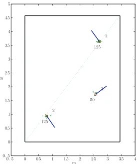
0. 5 0 0.5 1 1.5 2 2.5 3 3.5 4 0. 5 0 0.5 1 1.5 2 2.5 3 3.5 4 4.5 5 125 1 125 2 50 3 m m
Figure 2.2: Rectangular environment: CE-MCL iteration
2.3.2 Evaluation Criteria
Two indexes of quality have been chosen to evaluate the correctness of the algo-rithm: the percentage of estimation failures and the entropy measurement of the particle set. The first one gives information about the reliability and the accu-racy of the solution, the second one, coming from the information theory [140], provides a measurement of the uncertainty for a given random, and it is defined as: H(χ) = n X i=1 pilog2( 1 pi )
where, pi is the probability of the i-th outcome for a given event χ. In this context, entropy can be properly applied to give an evaluation of the persistence of the diversity among particles.
2.3.3 Simulations
Simulations were performed to investigate the algorithm capability to carry on the multi-hypothesis. Fig. 2.2 shows a typical CE-MCL iteration step for the rectan-gular environment. Points (green) represent particles, whereas circles (red) are located at the center of the mass of each cluster and, segments (blue) describe the mean orientation for all particles within each cluster. Due to the environmental symmetries, at each time-step at least two subset of hypotheses are maintained, in particular the ones located at the extreme of a segment splitting the environ-ment in two equal parts. Further, such behavior seems to be reasonable as sensor data support both locations, nothing that the laser beam range is limited to 8 m.
2.3.4 Robot in Real Environments
The robot was put into three different indoor office-like environments: • Entire building floor.
• T-shaped hall. • Corridor.
The first and second environments, shown respectively in Fig. 2.3 and Fig. 2.5 have been exploited to test the algorithm capability to solve both the global localization problem and the kidnapped robot problem. On the other hand, the third environment, shown in Fig. 2.7, has been exploited to investigate the local algorithm capability to converge within each cluster.
Entire building floor
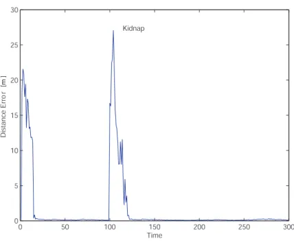
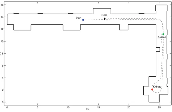
Fig. 2.3 shows a typical CE-MCL estimation result for the complex environment previously mentioned. Points (red) represent the most likely hypotheses at each time step, whereas the line (blue) represents the real robot path. In particular, S is the robot start point, K is the location at which the robot is kidnapped, R is the start point after the kidnap and finally, G represents the goal point of the robot. The algorithm has been able to find out a rough estimation of the robot
0 10 20 30 40 50 60 0 5 10 15 20 25 30 35 40 45 m m S K R G
Figure 2.3: Complex environment: CE-MCL estimation result
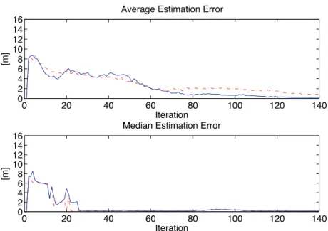
2.3 evidences the algorithm’s ability to realize when a kidnap occurs, thus re-localize the robot. The remaining noisy points, consequence of a temporary bad estimation, prove the algorithm’s tendency to explore the whole environment as well as to carry on the multi-hypotheses at each time step. Further, they might be easily removed, for instance relying on the kinematic model constraints of the mobile robot. The algorithm has been run several times in this environment to estimate the percentage of failures; the mean value settles around 30%, while the variance is ±4%. Fig. 2.4 shows the measurement of entropy for the experiment mentioned above. The red line represents the theoretical maximum entropy for the given set of particles, whereas the blue line describes the entropy during the algorithm execution, and the black line is its mean value. In order to maintain the diversity among the particle set, such value should be high. However, the algorithm should also be able to converge to the real robot location. For the CE-MCL algorithm, the mean value settles around an intermediate value, giving evidence of the algorithm’s aptitude to balance both needs.
0 500 1000 1500 2000 2500 2 3 4 5 6 7 8 9
Figure 2.4: Complex environment: CE-MCL entropy measurement
T-shaped hall
Fig. 2.5 shows a typical CE-MCL estimation result for such environment. The presence of structural ambiguities along with the noisiness of laser readings, due to the nature of glass, make the localization problem more difficult. Despite the fact that the accuracy of the estimation is lower than the previous experiment,
and the percentage of failures is markedly higher (mean value 40%, variance ±5%) the algorithm has been able to localize the robot, even under these critical conditions. Fig. 2.6 shows the measurement of entropy for this environment. As
0 2 4 6 8 10 12 14 16 18 20 0 2 4 6 8 10 12 14 16 18 m m
Figure 2.5: T-shaped environment: CE-MCL estimation result
in the previous experiment, the value settles around the median value, proving the algorithm’s ability to maintain the diversity among the particles set.
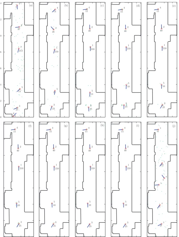
Corridor
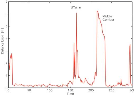
Fig. 2.7 shows a sequence of CE-MCL iterations for the corridor. This sequence of images describes the algorithm behavior between two resampling steps. In par-ticular, when the first resampling occurs (a), the algorithm recognizes six clusters (the last one is the collection of noisy points) with a visible dispersion for the el-ements within the environment. The following iterations point out the CE-MCL tendency to centralize the hypotheses around the center of mass of each cluster. Moreover, after few time-steps, clusters are coarsely located along a line crossing the corridor. This deployment underlines the algorithm tendency to maintain only the most likely hypotheses after a full exploration of the environment. Two aspects of interest have been considered to study the convergence of particles within each cluster: a measure of similarity and the state variables variance. From a mathematical standpoint, both the state space variables analysis and the measurement of entropy give evidence of these considerations. Fig. 2.8 shows a
100 200 300 400 500 600 700 800 900 1000 2 3 4 5 6 7 8 9 max entropy
Figure 2.6: T-shaped environment: CE-MCL entropy measurement
typical variance trend within a cluster for all three state variables: peaks indicate the resampling effect, whereas slopes give evidence of the algorithm aptitude to make particles converge within each cluster. Fig. 2.9 exhibits a typical measure-ment of entropy within a cluster: the trend is similar to the previous one due to the relationship among these concepts, when restricted to a single cluster. 2.4 Considerations
In this chapter an enhanced Monte Carlo Filter has been presented to deal with the localization problem: the Clustered Evolutionary Monte Carlo Filter (CE-MCL). This algorithm has been conceived to overcome the classical Monte Carlo Filter drawbacks. This goal has been achieved taking advantage of an evolu-tionary approach and a clustering method. In particular, the former has been exploited to quickly find out local maxima, whereas the latter, being dynami-cal, helps to obtain an effective exploration of the environment. The ability to provide a smart partition set of the research space along with the guarantee to converge within each subset, make the algorithm able to solve the localization problem and maintain the multi-hypotheses. Note that the combined use of clus-ter+genetic offers several interesting advantages. At local level, being the size of research space smaller, the localization of the best solution is faster and the probability to stall on a suboptimal solution is lower. At global level, being the clustering dynamical and data-driven, an implicit parallelization of the research is possible and a better coverage of the environment is obtained, focusing the
0 2 4 6 8 10 12 14 213 1 37 2 25 3 11 4 13 5 1 6 210 1 38 2 23 3 14 4 15 5 210 1 40 2 25 3 12 4 13 5 210 1 40 2 25 3 15 4 10 5 210 1 40 2 25 3 15 4 10 5 210 1 40 2 25 3 15 4 10 5 210 1 40 2 25 3 15 4 10 5 210 1 40 2 25 3 15 4 10 5 210 1 40 2 25 3 15 4 10 5 226 1 28 2 16 3 14 4 7 5 9 6 (a) (b) (c) (d) (e) (j) (i) (h) (g) (f)
Figure 2.7: Corridor-like environment: CE-MCL sequence of iterations
attention where the probability to find out the real robot pose is higher. Exhaus-tive analyses have been performed on the robot ATRV-Jr manufactured by the IRobot, with the employment of several environments, to prove the effectiveness of the proposed algorithm. In particular, two different kinds of experiments have
Figure 2.8: Corridor-like environment: CE-MCL variance
Figure 2.9: Corridor-like environment: CE-MCL entropy measurement
been considered: the first one has proved the algorithm ability to solve the global localization problem, even when a kidnap occurs; the second one has given evi-dence of the algorithm tendency to converge within each cluster and to guarantee an efficient exploration of the environment. Such analyses have shown the im-portant role of the dynamical spatial clustering to provide an effective partition of the research space on which apply the evolutionary action. Therefore, the CE-MCL can find out local-maxima, guarantee a convergence to the most likely hypotheses, maintain the diversity among particles and localize the robot.
A Spatially Structured Genetic Algorithm
In this chapter a novel approach based on spatially structured genetic algorithms is proposed. This approach takes advantage of the complex network theory for the spatial deployment of the population. In fact, modeling the search space with complex networks and exploiting their typical connectivity properties, results in a more effective exploration of such space. On the other hand, the introduction of spatial structures in evolutionary algorithms helps to create evolutionary niches. Since niches represent regions in which particular solutions are preserved, a nat-ural way to maintain the multi-hypothesis is achieved. The approach originally developed for the single-robot context has been successively extended to deal with the multi-robot context. A technique for integrating the information exchanged by robots anytime they meet is proposed with the aim of extending their sensory capabilities.
3.1 Theoretical Background 3.1.1 Complex Networks
Complex Networks are graphs of nodes or vertices connected by links or edges, currently used to describe many natural or artificial systems: the brain, for in-stance, can be modeled as a network of neurons, and the Internet as a complex network of routers and computers linked by several physical means. From the beginning, complex networks have been investigated by the graph theory com-munity, who proposed several models, such as regular and random graphs; since then several other communities have been interested in this topic. Today, a main research issue is to figure out the relationship between structural and dynamic properties of the networks.
Regular graphs, introduced to describe systems made of a limited number of nodes, were revealed to the research community to be inadequate with the appearance of large-scale networks. This has lead the community to focus their attention on random graphs. According to [120], once the probability p of having a connection among pairs of nodes is fixed, a random graph with N nodes and
about pN (N − 1)/2 links, can be obtained randomly selecting a pair of nodes and linking them with such probability p. This model has been extensively used since particular properties of complex networks, such as the small-world property or the scale-free one, have been discovered.
To better understand such properties, some basic concepts about complex networks have to be introduced: the average path length, the cluster coefficient and finally the degree distribution.
The average path length L of the network is the mean distance between two nodes, averaged over all pairs of nodes, where the distance between two nodes is defined as the number of the edge along the shortest path connecting them.
The cluster coefficient C of the network is the average of Ci over all nodes i, where the coefficient Ci of node i is the average fraction of pairs of neighbors of the node i that are also neighbors of each other.
The degree distribution of the network is the distribution function P (k) describ-ing the probability that a randomly selected node has exactly degree k, where the degree k is the number of links a node owns.
Watt-Strogatz Barabasi-Albertµ
Figure 3.1: Watt-Strogatz and Barab´asi-Albert models with 30 nodes
From a formal point of view, regarding these basic properties, several com-plex network models can be correctly defined. Regular graphs, for instance, are characterized by a high cluster coefficient, approximately C ∼= 3/4 and a large average path tending to infinity as N → ∞. Random graphs have a low cluster coefficient, approximately equal to the probability p defined above, and a short average path Laver ∼= lnN/(pN ). In [154] the Small-World model is proposed to better describe real systems. It shows properties of both the regular and random graphs, such as a high cluster coefficient and a short average path, underlining the fact that, in reality, the circle of acquaintances of people is not only restricted to their neighbors. In [15] the Scale-Free model is presented. This model, relying on the power-law degree distribution, overcomes the limitations of the previous ones through a hierarchical description of nodes. As a consequence, in a scale-free network preferential attachments are possible. This model, for instance, turns out to be very useful to describe airline routing maps.
Two examples of the above described networks are reported in Fig. 3.1; for a complete overview of complex networks the [153] is suggested.
3.1.2 Spatially Structured Genetic Algorithms
Spatially Structured Genetic Algorithms (SSGAs) represent a special class of Genetic Algorithms (GAs), which are described in Appendix B, where the pop-ulation is spatially distributed with respect to some discrete metric. SSGAs are characterized by different properties than standard GAs, such as the capability to preserve the diversity or to create evolutionary niches.
SSGAs can be properly described by exploiting the graph theory. In this context, given a population P ={p1, . . . , pn} and a graph G = (V, M), where V = {v1, . . . , vn} is the set of vertices and M = {(i, j) = 1 : ∃ link between i and j} is the incidence matrix, a Spatially Structured Genetic Algorithm can be obtained by defining an isomorphismF(·) from P to V so that:
F : P → V (3.1)
Therefore, a SSGA is a variation of a Simple Genetic Algorithm (described in Appendix B) where selection is performed by exploiting the topology of the graph underlying the population in spite of using the roulette wheel.
Note that, this formalization was already used to introduce the graph based genetic algorithms in [9]. Here, the idea was to prevent the loss of diversity by imposing geographical structure to the population to limit choice of crossover partners. Finally, a more comprehensive treatment of this class of genetic algo-rithms is given in [146]
3.2 The proposed spatially structured genetic algorithm over complex net-works
The proposed SSGA provides a framework for both single robot and multi-robot localization problem. It takes advantage of the complex network theory for the deployment of the population. Giving such a structure to the population leads to several interesting advantages, such as the capability to carry on the multi-hypothesis paradigm.
In this context, a chromosome encodes the state of the robot, represented through its position and orientation (x, y, θ). From an algorithmic standpoint, a SSGA reflects the classical SGA schema described in Appendix B with a spe-cialization regarding the structure of the population. In the initialization step, a population is randomly generated and its individuals are connected to obtain a complex network, typically small-world and scale-free. At each epoch k, the pop-ulation evolves dynamically, according with the kinematic model of the robot and the input applied, maintaining the topology of the network. Such a topology is exploited during the selection phase, which is trivially realized picking up all the
pairs of linked elements. In the reproduction stage the mating rules represented in Table 3.1 are used to choose the probabilistic transition operator.
To apply the mating rules, each individual is labeled with the tag high or low, computed by means of a comparison between the fitness of the individual itself and the average fitness of the population.
Table 3.1: Mating rules
Node 1 Node 2 Action Basic principles
Low Low Both self-mutate Mutation
High Low Node 2 is replaced with Elitism and
a Mutation of Node 1 Mutation
Low High Node 1 is replaced with Elitism and
a Mutation of Node 2 Mutation
High High The lower is replaced with Elitism and
the Crossover on the two Crossover
Regarding the probabilistic transition operators: crossover picks up two ele-ments and performs a convex combination of them with probability pcross, while mutation picks up an element and modifies its chromosoma, inversely propor-tional to its fitness, with probability pmutat.
3.2.1 Independent Evolution
Anytime a robot is moving and no other one is within its communication range, the only information available is the data coming from its sensors. Therefore, each robot performs an independent evolution computing a measure of similarity between data coming from a real robot and the expected one computed for a given hypothesis. Specifically, the fitness function of an individual i weights the compliance between the exteroceptive measurements (zk) retrieved by the robot and the ones (ˆzk) expected by the individuals itself
Φi(zk, ˆzk) = 1 L L X j=1 1 √ 2πσe −(zjk−ˆzj k)2 2σ (3.2)
where σ is the confidence of the sensor and L is the number of measurements considered. The pseudo-code in algorithm 3 shows a possible implementation schema for a generic step k of independent evolution for the proposed SSGA. 3.2.2 Cooperative Evolution
The same approach holds when considering multi-robot localization. In this case, although for each robot a population is initialized and lets evolve independently, a collaboration can be set-up any time when robots meet. The key idea is to integrate the observations coming from the components in such a way that the sensory system capability of each robot is extended. In order to achieve that, the relative position and orientation of the robots in the team are assumed available along with the sensor data, while the fitness function is augmented in the following
Algorithm 3: The proposed SSGA - iteration k
Data: Population of size n: {V = {pj,k}, M }, Φ(·), e(·) Result: V = {pj,k+1}
/* Average Fitness Evaluation */
Φaver=Pni=1Φ(pi,k)/n 1
/* Incidence Matrix Selection */
fori=1 to n do 2 forj=i to n do 3 if M (i, j) = 1 then 4
switchCompare({Φ(pi,k), Φ(pj,k)}, Φaver) do 5 caseHigh-High 6 if Φ(pi,k) > Φ(pj,k) then 7 pj,k = Crossover(pi,k, pj,k) 8 else 9
pi,k = Crossover(pi,k, pj,k) 10 end 11 caseHigh-Low 12 pj,k = M utation(pi,k) 13 caseLow-High 14 pi,k = M utation(pj,k) 15 caseLow-Low 16
pi,k = M utation(pi,k) pj,k = M utation(pj,k) 17 end 18 end 19 end 20 end 21 {pj,k+1} = {pj,k} 22 /* Kidnap Detection */
if Kidnap Condition then 23 Spreading Action 24 end 25 way Φi(zk, ˆzk) = 1 L L X j=1 1 √ 2πσe −(zjk−ˆzj k)2 2σ + R X r=1 1 Lr Lr X l=1 1 √ 2πσe −(zlk −ˆzlk)2 2σ (3.3)
where R is the number of the robot of the team in the viewing area and Lr the number of sensor of the r–th robot. The second addendum weights the compli-ance of the measurement of the team formation with respect to the formation replicated around the i-th individual. In this way the localization algorithm re-sults completely distributed and collaboration is possible even when robots move. Cooperation turns out to be fundamental in reducing the perceptual aliasing, as the more data available the higher the probability to converge to a single loca-tion. It is well known that a genetic approach helps to maintain a population of multiple hypotheses. In particular, SSGA, due to their convergence proprieties, usually maintain equally probable hypotheses and, in presence of sufficient and not ambiguous information, converge to a neighborhood of the solution. This fast takeover is related to the structure of the space of interactions and can be
exploited monitoring the formation of a single cluster.
Although the algorithm is able to solve the global localization problem with a proper random initialization, an additional strategy, able to perceive when a kidnap occurs, is required in order to spread the population over the search space again and then re-localize the robot. In this work, the fitness function Φ(·) and the edge function e(·), i.e., the fraction of potential mating couples (couples with different genotypes) over the network (the number of links) [9], are used to trigger the spreading action. The edge function gives an evaluation of the dispersion of the population. Specifically for a well-localized robot, a high percentage variation of the fitness along with a considerable dispersion of the population (a high value of the edge function), are reliable symptoms of a kidnap.
3.2.3 Computational Complexity
The analysis of the computational complexity is important to evaluate the ca-pability of an algorithm to run online. For this reason, a detailed theoretical investigation along with an empirical validation of the obtained results has been performed. The pseudo-code proposed in Algorithm 3 presents two nested loops in which the dominant operation is the fitness evaluation whose complexity for each element of the population is O(M), where M is the number of segments describing the environment. As a consequence, the overall complexity for this naive implementation results in O(M · N2), where N is the size of the popula-tion. However, a more effective implementation can be provided by observing that:
• The fitness value for each element of the population can be stored during the evaluation of the average fitness function (algorithm 3 - line 1).
• A mating rule is applied only when a link is available between two elements (algorithm 3 - line 4).
This way the complexity can be significantly lowered. In fact, pre-evaluating the fitness and storing it reduces the complexity of the dominant operation within the nestled loop to a constant factor O(1). On the other hand, the two loops can be replaced with a vector indexing all the couples with a link. Since for the considered topologies the number of links is proportional to the size of the population, i.e., (k−1)·N/2 with k node degree of each node, the over complexity of the algorithm is reduced to O(k · N · M) = (k−1)·N ·M2 .
The first element is the cost of scanning all the couples with a link, while the second is the cost of evaluating the fitness for the whole population.
3.3 Performance Evaluation
The proposed Spatially Structured Genetic Algorithm has been extensively in-vestigated in both simulated environment and with real robot data. Real