DIPARTIMENTO DI FISICA E ASTRONOMIA
Dottorato di ricerca in Astronomia
Ciclo XXVIII
Non-thermal emission in
High Frequency Peaked blazars towards
the Square Kilometer Array era
Relatore:
Chiar.mo Prof.
Gabriele Giovannini
Co-Relatori:
Dott. Marcello Giroletti
Dott.ssa Monica Orienti
Coordinatore:
Chiar.mo Prof.
Lauro Moscardini
Tesi di Dottorato di:
Rocco Lico
Settore Concorsuale: 02/C1 Astronomia, Astrofisica, Fisica della Terra e dei Pianeti Settore Scientifico-Disciplinare: FIS/05 Astronomia e Astrofisica
in the framework of the research activities
Introduction 1
1 The blazar family 7
1.1 Active Galaxies . . . 7
1.1.1 Radio-loud AGNs . . . 10
1.2 The blazar properties . . . 12
1.2.1 Variability . . . 12
1.2.2 Broadband spectral properties . . . 14
1.2.3 The blazar’s divide . . . 18
1.2.4 The blazar sequence . . . 22
1.3 High Synchrotron Peaked blazars . . . 24
2 Physical and geometrical properties of sources in relativistic motion 29 2.1 Doppler boosting . . . 30
2.2 Brightness asymmetries . . . 34
2.3 Brightness temperature . . . 35
2.4 Apparent transverse speed . . . 36
3 Observing instruments and techniques 39 3.1 Radio interferometry . . . 39
3.2 Towards the future: Square kilometer Array . . . 44
CONTENTS
3.3.1 Theγ-ray sky and the Fermi-LAT catalogs . . . 48
4 VLBA observations of Fermi-LAT sources above 10 GeV 51 4.1 The first Fermi-LAT catalog of sources above 10 GeV . . . . 52
4.2 Sample selection . . . 57
4.2.1 Observations and data reduction . . . 60
4.3 VLBI properties and detection rate . . . 64
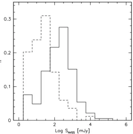
4.4 Flux density distribution . . . 68
4.5 High energy properties . . . 70
4.6 Proposed counterparts for unassociated sources . . . 71
4.7 Brightness temperature . . . 73
4.8 Summary . . . 74
5 Correlation analysis for the first Fermi-LAT catalog of sources above 10 GeV 77 5.1 Connection between radio andγ-ray emission in blazars . . . 77
5.2 1FHL blazars in the northern hemisphere . . . 79
5.3 Correlation analysis between radio andγ-ray emission . . . 87
5.3.1 The method of surrogate data . . . 88
5.3.2 Results . . . 90
5.4 Discussion . . . 95
6 Physical and kinematic properties of the HSP blazar Markarian 421 99 6.1 Observations . . . 101
6.2 Results . . . 103
6.2.1 Images . . . 103
6.2.2 Model fits . . . 103
6.2.3 Flux density variability . . . 111
6.2.4 Apparent speeds . . . 112
6.3 Discussion . . . 115
7 Polarization properties andγ-ray connection in Mrk 421 119 7.1 Polarization calibration . . . 120
7.1.1 Determination of uncertainties . . . 123
7.2 Fermi-LAT data: selection and analysis . . . 124
7.3 Results . . . 127
7.3.1 Images and morphology . . . 127
7.3.2 Radio light curves and evolution of polarization angle . . 130
7.3.3 Faraday rotation analysis . . . 134
7.3.4 γ-ray light curves from Fermi data . . . 137
7.3.5 Correlation between radio andγ-ray data . . . 139
7.4 Discussion . . . 141
7.4.1 Possible radio andγ-ray connection . . . 141
7.4.2 EVPA variation and magnetic field topology . . . 145
Conclusions 149
Introduction
In the class of Active Galactic Nuclei (AGN), blazars are the most extreme ob-jects. They show a pair of prominent relativistic plasma jets closely aligned with our line of sight, powered from the gravitational potential of a super massive black hole (with a mass up to∼ 109M
⊙), accreting matter and gas from the surrounding
medium. Their emission is mainly non-thermal and it is detected throughout the electromagnetic spectrum, with a typical two-humped spectral energy distribution (SED). Due to their peculiar geometry, these jet structures are detected at extreme cosmological distances thanks to the strong Doppler boosting effects produced by the bulk relativistic motion. For this reason they are among the most powerful objects in the Universe.
Understanding the details of the production mechanism and the fueling pro-cesses of the relativistic jets is crucial to understand the physics of the matter in extremely compact states, the physics of high energy plasma and the role of mag-netic fields. In recent years, the field ofγ-ray astrophysics has greatly developed, thanks to the advent of the Large Area Telescope (LAT) on-board the Fermi satel-lite, which detects γ rays in the energy range between ∼20 MeV and ∼300 GeV, and of ground-based Cherenkov telescopes which allow us to study very-high en-ergy (VHE, E > 0.1 TeV) γ rays. These instruments have clearly revealed that blazars dominate the census of theγ-ray sky.
Exploring the possible correlation between radio andγ-ray emission is a cen-tral issue to understand the blazar emission processes, and several works and ob-serving campaigns were dedicated to this topic (e.g. Kovalev et al. 2009; Ghirlanda
et al. 2010; Giroletti et al. 2010; Ackermann et al. 2011a; Mufakharov et al. 2015). However, while a strong correlation between radio andγ-ray emission in the energy range 100 MeV–100 GeV was clearly demonstrated (Ackermann et al. 2011a), the possible correlation radio-VHE still remains elusive and unexplored. Any possible physical implication based on the relation between the two bands has remained hidden, mainly due to the lack of an homogeneous coverage of the VHE sky. Currently, VHE observations of blazars are conducted by imaging at-mospheric Cherenkov telescopes (IACTs), which mainly operate in pointing mode with a limited sky coverage, and in general they observe sources in a peculiar state. All of these limitations introduce a strong bias in VHE catalogs, and it is difficult to assess any possible radio-VHE correlation.
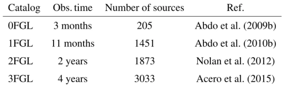
At present, the First Fermi-LAT Catalog of Sources above 10 GeV (1FHL, Ackermann et al. 2013), represents the best resource for addressing the connection between radio and hardγ-ray emission, approaching and partly overlapping with the VHE band. The 1FHL catalog is based on LAT data accumulated during the first 3 years of the Fermi mission. Since Fermi operates in sky survey mode, the 1FHL provides us, for the first time, a large, deep and unbiased sample which is ideal to gatherγ-ray data in the energy range 10-500 GeV.
Hard blazars are generally of the High Synchrotron Peaked (HSP) type, with the synchrotron SED component peaking at ν > 1015 Hz, characterized by low
Compton dominance, low synchrotron luminosity, and peculiar very long baseline interferometric (VLBI) properties: their parsec scale jets are less variable in flux density and structure than in other blazars, and in general the inferred Doppler factors are far from the extreme values required at higher frequencies. About 40% of 1FHL blazars are of HSP type and the investigation of their properties provides us with details about the blazar sequence (Fossati et al. 1998), and the interaction of VHE photons with the extragalactic background light.
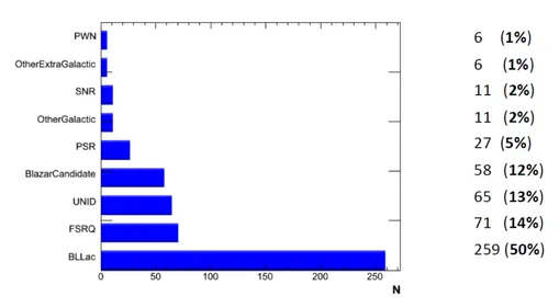
In this thesis work we will explore and discuss the properties of 1FHL sources, considering both blazars and the non negligible fraction of still unassociated
gamma-Introduction
ray sources (UGS, 13%). We perform a statistical analysis of a complete sample of hard γ-ray sources, included in the 1FHL catalog, mostly composed of HSP blazars, and we present new VLBI observations of the faintest members of the sample. The new VLBI data, complemented by an extensive search of the archives for brighter sources, are essential to gather a sample as large as possible for the assessment of the significance of the correlation between radio and VHE emission bands.
UGS constitute 13% of the 1FHL, and about the 30% of every other Fermi catalog. Are these UGS just unrecognized blazars or more exotic objects? Do they show the same radio vs. high energy γ-ray connection found for the other γ-ray sources? With the new VLBI observations of the present work we will be able not only to definitively confirm the blazar nature of some 1FHL sources, but we will propose a reliable association for some UGS with a high significance.
After the characterization of the statistical properties of HSP blazars and UGS, we use a complementary approach, by focusing on an intensive multi-frequency observing VLBI andγ-ray campaign carried out for one of the most remarkable and closest HSP blazar Markarian 421 (Mrk 421).
In general HSP blazars show a violent variability on short timescales, from the order of years to few days, that is sometimes accompanied by the ejection of superluminal blobs. This violent activity suggests that the central engine is not sta-tionary, and, due to the very short timescales involved, this behavior can be related to rapid changes in the magnetic field. For this reason, we investigate the inner jet structure of Mrk 421 on the finest possible linear scales: in radio, we can do this directly with parsec-scale imaging, by means of a one-year multi-frequency VLBI monitoring, both in total and in polarized intensity; inγ rays, we infer information on small spatial scales through the construction and analysis of a weekly-binned light curve. We constrain the geometry and kinematics of the jet by studying the evolution of shocks that arise in it and we estimate some important quantities and parameters such as the jet viewing angle, the Doppler factor and the
bright-ness temperature. Thanks to the electric vector position angles (EVPA) and the Faraday rotation analysis we obtain information about the magnetic field topol-ogy both in the core and in the jet region. Finally, we compare the information gathered from the radio and theγ-ray data.
From the study and results of the present thesis work it emerges how much important it is to achieve a higher sensitivity to understand the physical mecha-nisms occurring in hard γ-ray blazars. In general, faint Fermi-LAT sources are also faint radio sources. The weakestγ-ray sources detect by Fermi have 1.4 GHz flux densities of few mJy, and the unassociated ones are expected to be fainter.
The Square Kilometer Array (SKA), which is a new generation revolutionary aperture synthesis radio telescope, with its exceptional sensitivity (at µJy level) and large field of view, will be the ideal instrument to better characterize these sources and to disentangle among the low frequency candidate counterparts. In particular, the synergy between SKA and the new generation Cherenkov tele-scope Array (CTA), will provide us with the perfect chance to investigate the possible radio-VHE emission connection and to identify and reveal the nature of the unidentified Fermi high energy sources.
The thesis is laid out as follows: the first three Chapters are devoted to an intro-duction of the science topics and observing techniques: in Chapter 1 we introduce and describe the properties of AGNs in general and of blazars in particular; in Chapter 2 we describe some relativistic effects which play an important role in the observational properties of blazar jets; in Chapter 3 there is an introduction about the observing instruments and techniques used in this work: radio interferometry and VLBI technique, the Large Area Telescope on board the Fermi satellite and the new generation aperture synthesis radio telescope SKA.
Chapters 4 and 5 are focused on the 1FHL sample: in Chapter 4 we present our new VLBI observations for the faintest 1FHL sources; in Chapter 5 there are the results about the radio andγ-ray emission correlation analysis together with the correlation significance assessment.
Introduction
The last two Chapters deal with the one-year broadband monitoring of the HSP blazar Mrk 421: Chapter 6 contains results about the total intensity analysis of the multi-epoch multi-frequency VLBI monitoring; in Chapter 7 we report on the polarimetric parsec-scale analysis, theγ-ray light curve, and their connection. Throughout this work, we use aΛCDM cosmology with h = 0.71, Ωm = 0.27,
and ΩΛ = 0.73 (Komatsu et al. 2009). The radio spectral index is defined such that S (ν) ∝ ν−α and the γ-ray photon index Γ such that dNphoton/dE ∝ E−Γ. All
Chapter 1
The blazar family
1.1
Active Galaxies
About 1% of the galaxies in the Universe show features that are markedly different with respect to those observed in the “normal” ones. These galaxies have a typical luminosity that is L∼ 1047− 1048erg s−1, i.e. about three orders of
magnitude higher than what is found in a typical galaxy, and it cannot be solely attributed to the emission of stars, gas and dust. The huge amount of energy originates in the central compact region of these galaxies, called Active Galactic Nucleus (AGN), and the host galaxy is called active galaxy.
Under the name of active galaxies various sub-classes of objects are included (e.g. quasars, Seyfert galaxies, radio galaxies, blazars), which differ from each other in brightness, morphology, distance, variability and polarization degree.
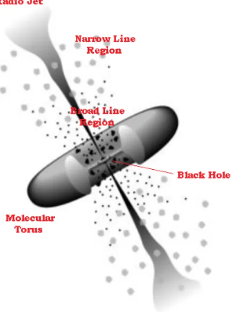
However, some features seem to be common to all the different AGN classes, and a standard unified model was built. The basic scheme of this model, as re-ported in Fig.1.1, foresees the presence of a super-massive black hole (SMBH, with a mass of∼ 106−10M⊙), which acts as a central engine. Due to the gravity of the SMBH, the surrounding gas falls towards the center, dissipating angular momentum due to viscosity and turbulent motions, and forms an accretion disk
Figure 1.1:Schematic representation of the current AGN paradigm. Image adapted from Urry & Padovani (1995).
around the central engine, extending for about 10−3pc (Krolik 1999). The accre-tion disk is responsible of the thermal emission in the optical-UV wavebands. In addition, above the disk, a hot corona forms, in which X-ray photons are produced by means of inverse Compton (IC) scattering of optical-UV photons coming from the disk.
Above the disk, at∼ 0.01−0.1 pc from the core, there is a region known as the broad line region(BLR), formed by moving and turbulent gas clouds which can reach electron densities of the order of 108−11cm−3. Being close to the black hole, these clouds have high rotational speeds (∼ 500 − 104km s−1) and produce broad
lines in the observed spectrum, because of Doppler effect. Beyond this region, between∼ 1−100 pc from the core, there is an optically thick dusty torus, which produces IR emission by reprocessing the optical/UV photons coming from the disk and re-radiating them at longer wavelengths.
1.1. Active Galaxies
Figure 1.2: Schematic representation of the broadband continuum spectral energy dis-tribution of AGNs. The main components are: the infrared bump, which is thought to be re-radiated emission from the dust torus; the Big Blue Bump (UV/Optical) from thermal emission from the accretion disk; and the X-ray emission from Comptonization of disk photons in a hot corona. Image from Elvis et al. (1994).
region of low-density clouds (electron densities of the order of 104−6cm−3), with
rotational speeds lower than∼ 103km s−1, producing narrow emission lines. This
outer region is known as narrow line region (NLR) and is responsible for the forbidden lines observed in the spectrum (i.e. emission lines that in environments with higher densities would be suppressed by collisional processes).
A schematic representation of the broadband continuum emission spectrum of AGNs, with the contribution from the different components, is shown in Fig. 1.2. It is clear how this unisotropic structure is highly directional (see Fig. 1.3): the observed spectrum and features strongly depend on the angle that this structure forms with the line of sight (Urry & Padovani 1995). In particular, when the molecular torus intercepts the line of sight, it can hide the emission of the internal regions (disk emission and emission lines produced by the BLR).
It should be noticed that this is a basic model. Although it could not take into account all the observational properties of the whole AGN class, it successfully
Figure 1.3: A cartoon of the AGN unified model from Beckmann & Shrader (2012). Depending on the viewing angle different type of objects are seen. Radio-loud and radio-quiet objects are represented in the top and in the bottom part of the image, respectively.
explains most of them. However, there are some clues indicating that also some intrinsic different properties are responsible of the AGN diversification. Some of the main discriminant parameters are thought to be the mass accretion rate onto the SMBH and the SMBH spin (e.g. D’Elia & Cavaliere 2001; Chiaberge & Marconi 2011).
1.1.1
Radio-loud AGNs
About 10% of the entire AGN population form bipolar and powerful jet struc-tures, originating in the central region along the rotation axis of the black hole (Peterson 1997). These jets, which can extend from a few pc up to several Mpc, are mainly made of relativistic plasma, whose particles are accelerated and, by interacting with the radiation field and the magnetic field, produce part of the ob-served spectrum. These sources are classified as radio-loud sources, which means that the ratio of flux densities in the radio at 5 GHz and in the optical B-band in the source rest frame is higher than 10 (Kellermann et al. 1989).
1.1. Active Galaxies
Table 1.1: FRI and FRII properties.
FRI FRII
log P1.4 < 1024.5Watt Hz−1 log P1.4 > 1024.5Watt Hz−1
diffuse jets highly collimated jets
no hot spots bright hot spots
edge-darkened edge-brightened
weak optical emission lines strong optical emission lines
Radio galaxies are the most common radio-loud AGNs. When we talk about radio galaxies, we intend extragalactic and spatially resolved radio sources, usu-ally associated with giant elliptical galaxies, whose broadband spectrum is dom-inated by non-thermal emission. Their structure includes two radio jets, and in the most powerful ones, bow shocks create extended and diffuse structures called
radio lobes.
The family of radio galaxies is further divided into two sub-classes, depending on the radio power and morphological features. The astronomers Fanaroff and Riley in 1974 noticed that when the radio power at 178 MHz of a radio galaxy is higher than∼ 1025Watt Hz−1Sr−1, there is a change in the source morphology.
The fainter radio sources are called Fanaroff-Riley Type I (FRI), whereas the more powerful ones are called Fanaroff-Riley Type II (FRII).
From a morphological point of view, in FRI radio galaxies jets appear symmet-rical, bright and diffuse, while in FRIIs there are well collimated, asymmetric and low-luminosity jets. In FRIIs the jet ends in a compact and bright region called hot
spot at the edge of the lobes (edge-brightened), while in FRIs hot spots are absent
and the lobes appear brighter in the inner part (edge-darkened). These differences may be related to the radiative efficiency of the accretion flow: in FRIIs the ac-cretion is more efficient than in the FRIs (Ghisellini & Celotti 2001). The main properties and differences between FRI and FRII radio galaxies are summarized in Table 1.1.
Radio-loud AGNs with their jet structures closely aligned to the line of sight form the class of the so called blazars. In these objects the Doppler boosting effect plays a major role and produces high variability throughout the electromag-netic spectrum, high degree of radio and optical polarization and high brightness temperature (see Sect. 2). Moreover, apparent superluminal motions of jet com-ponents can be detected with high angular resolution observations. Due to this peculiar geometrical configuration, blazars represent the most extreme AGN fam-ily and they are less than 5% of the entire AGN class.
Blazars are the main topic of this thesis and their properties will be extensively discussed in Sect. 1.2.
1.2
The blazar properties
The blazar family consists of two sub-classes: BL Lacertae objects (hereafter BL Lacs) and Flat Spectrum Radio Quasars (hereafter FSRQs). Historically, they are classified into FSRQs and BL Lacs on the basis of their optical properties: FSRQs show broad and strong emission lines in their optical spectra while the optical spectra of BL Lacs are almost featureless.
In this section we will describe the main properties of blazars.
1.2.1
Variability
The study of the variability plays an important role for understanding the source physical state and for estimating the size of the emitting regions.
Blazars are among the most variable extragalactic objects, both in amplitude and timescales. Before entering into discussion, we should remind that when we speak about variability we intend a sudden increase in the emission intensity with respect to a flat or a slowly variable background, followed by a gradual decrease to the initial value. These intensity variations, called outbursts, usually are not regular (no evidence of any systematic periodicity have been established so far)
1.2. The blazar properties
and occur over timescales that can range from several years to a few days. In some cases outbursts can be accompanied by structural changes in the source (e.g. Orienti et al. 2013; Jorstad et al. 2013).
After decades of efforts in the study of relativistic jets, many issues still remain elusive, as the jet launching mechanism and acceleration, the precise location of the high energy emitting region and the jet structure itself. Among the various scenarios proposed for explaining the observed variability, there is the so called "shock-in-jet" model (Marscher & Gear 1985) which foresees that a shock orig-inates from a disturbance in the nuclear region and expands downstream across the jet region, producing both radio and high energy emission. On the other hand, there are pieces of evidence of relativistic jets showing a transverse velocity struc-ture, in which the radio and the high energy emission originate in different regions (e.g. Ghisellini et al. 2005; Gabuzda et al. 2014).
With the argument of causality, from the observed variability it is possible to estimate the size of the emitting region. In other words, given a source of radiation of size ∆d, from an external reference system, it cannot be measured variability on time scales which are shorter than the time that the light would take to travel a distance equal to the size of the source (∆d < c∆t).
Extremely short variability timescales, and therefore small sizes, imply high brightness temperature (TB) values, within the synchrotron model framework. The
brightness temperature, which is a different way of expressing the radiated power, is defined as the temperature that a black body should have to radiate the observed brightness. We can write TBas a function of the source angular size (e.g. Piner et
al. 1999; Tingay et al. 1998):
TB= 1.22 × 10¹²
S (1+ z)
abν2 K (1.1)
where S is the flux density of the component measured in Jy, a and b are the full widths at half maximum of the major and minor axes respectively of the com-ponent measured in mas, z is the redshift, andν is the observation frequency in GHz.
The brightness temperature can also be written as a function of the variability timescale (e.g. Hovatta et al. 2009):
TB,var = 1.548 × 10⁻³²
∆Smaxd2L
ν2τ2(1+ z)1+α K (1.2)
whereν is the observed frequency in GHz, z is the redshift, dL is the luminosity
distance in meters, ∆Smax is the difference between the maximum and the
mini-mum value of the core flux density in Jy,τ is the variability timescale and α is the spectral index.
For small values ofτ, the observed TBcan reach high values, in some cases
ex-ceeding the IC process critical threshold value of 1012K (Kellermann &
Pauliny-Toth 1969). When the brightness temperature exceeds this limit, the Compton brightness dominates over the synchrotron brightness, and because of the rapid en-ergy losses due to inverse Compton effect the source quickly cools down (Comp-ton catastrophe).
On the other hand, by fixing TB ≤ 1012K in Eq. 1.1 it is possible to obtain a
lower limit for the angular size of the source. In some cases, from this estimation, it emerges that the diameter of the source should be much larger than the value obtained from the observed variability. This apparent inconsistency is explained in the context of relativistic theories presented in Sect. 2.
1.2.2
Broadband spectral properties
In Astronomy, when we deal with multi-frequency studies, the standard way to represent spectra is by means of the Spectral Energy Distribution (SED). It consists in representing log(νFν) vs. log(ν), where ν is the photon frequency and
Fν is the energy flux per frequency unit. In other words, we represent the source power per natural logarithmic frequency intervals with the big advantage of di-rectly showing the relative energy output in each single frequency interval.
From the analysis of several blazar spectra, a universal trend in the log(νFν) vs. log(ν) plane was identified, represented by two non-thermal components. This
1.2. The blazar properties
Figure 1.4: Spectral energy distribution of Mrk 421 obtained with two one-zone synchrotron-self-Compton model fits, by using different minimum variability timescales:
tvar = 1 day (red curve) and tvar = 1 hr (green curve). For further details see Abdo et
al. (2011).
can be seen in Fig. 1.4 where the SED of the blazar Markarian 421 (Mrk 421) is shown. Two broad humps cover the entire electro-magnetic spectrum from radio to γ rays, whose peaks can lay at different energies, depending on the physical properties of the object that we are considering.
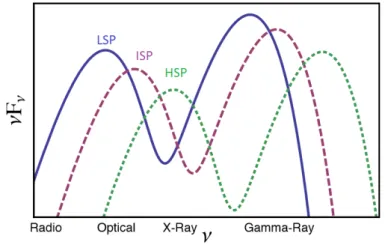
The low-frequency component, as suggested by the power law trend and the high degree of polarization observed in radio and optical bands, is due to syn-chrotron emission by relativistic electrons moving along the magnetic field lines. The synchroton hump peak (νS ynpeak) can be found in the spectral region extending from radio to soft X-ray energies, and it reflects the maximum energy at which particles can be accelerated (Giommi et al. 2012a). According to the conven-tion proposed by Abdo et al. (2010a), depending on theνS ynpeakposition, blazars are classified as: Low Synchrotron Peaked (LSP) withνS ynpeak < 1014Hz, Intermediate
Synchrotron Peaked (ISP) with 1014Hz< νS ynpeak < 1015Hz , and High Synchrotron Peaked (HSP) withνS ynpeak > 1015Hz (see Fig. 1.5). In general FSRQs are predomi-nantly LSP objects, while BL Lacs could be of all the three types.
The high-frequency component peaks from X-ray toγ-ray frequencies, in an energy range from keV to TeV. While there are many and stringent indications that the low-frequency component is due to synchrotron radiation, the origin of the high energy emission component is not so obvious. It is important to understand which kind of relativistic particles are responsible for the high energy component. There are two main families of models: the hadronic model, in which relativistic protons within the jet are the ultimate responsible for the observed emission, and the leptonic model, in which leptons play a dominant role.
According to hadronic models, protons within the jet interact with the sur-rounding photons, producing e±pairs, which by means of synchrotron processes, produce the high-frequency emission represented by the second hump in the ob-served spectrum (e.g. Mannheim 1993). However, being protons more massive than electrons, the acceleration efficiency is lower and they have longer cooling times. Moreover, protons require magnetic fields of the order of tens of Gauss to produce the observed emission.
On the other hand, leptonic models explain the high energy emission through IC scattering between relativistic electrons in the jet (the same ones responsible for the synchrotron emission) and surrounding low energy photons.
To date, no definitive indication has been found to discern between these two scenarios. However the following observational pieces of evidence favor the lep-tonic model for the high frequency emission:
• the similar trend of the two non-thermal humps points out that the parti-cles responsible for the high energy emission are the same producing the synchrotron emission at lower frequencies;
• in some objects, when one of the two peaks is higher or lower, the same behavior is then reflected in the other one;
• for a variability in the low frequency component, a subsequent instability in the high energy component is usually observed.
1.2. The blazar properties
Figure 1.5: Blazar classification according to the synchrotron peak (νS ynpeak) position in the Spectral energy distribution: Low Synchrotron Peaked (LSP) withνS ynpeak < 1014Hz, Intermediate Synchrotron Peaked (ISP) with 1014Hz< νS ynpeak < 1015Hz , and High Syn-chrotron Peaked (HSP) withνS ynpeak> 1015Hz.
This observational evidence is naturally explained by leptonic models, which easily reproduce the multi-frequency observed properties, while it is more difficult to conciliate them with hadronic models. Moreover, the TeV emission is better explained within the leptonic scenario: being the electrons less massive, it is easier to accelerate them by shocks to such high energies.
Regarding the scattered photons involved in the IC process, they may be the same photons produced by synchrotron emission within the jet (Synchrotron Self Compton model or SCC, Maraschi et al. 1992), or photons from external sources such as the accretion disk, the BLR and/or the dusty torus (External Radiation Compton Model or ERC, Dermer et al. 1992; Sikora et al. 1994; Ghisellini & Madau 1996; Sikora et al. 2008).
The density of the radiation field plays an important role in the physics of these peculiar objects: both components of the spectrum move to lower frequen-cies when the brightness of the radio source increases (see Fig. 1.5). Basically, all electrons are accelerated at similar energies. However, in the most powerful
sources (i.e. the most luminous) the photon density is higher, therefore relativistic electrons cool more efficiently, and as a consequence, the emission shifts to lower frequencies (Ghisellini et al. 1998).
From the above mentioned SSC model, in which the high energy emission is produced by IC scattering of the synchrotron photons, another important prop-erty emerges. The peak frequency of the low energy (LE) synchrotron component is related to the magnetic field intensity and the energy distribution function of electrons. On the other hand, the peak frequency of the high energy (HE) inverse Compton component is related to the radiation field intensity and the energy distri-bution function of electrons. Therefore, in the jet we expect that the ratio between the brightness of the LE and HE components reflects the ratio between the energy density of the radiation field and of the magnetic field.
1.2.3
The blazar’s divide
In this section we focus our attention on the main differences between the two blazar sub-groups, trying to understand if they are intrinsically different objects or if their differences are only apparent.
According to the optical classification of FSRQs and BL Lacs, for practical reasons, a threshold rest-frame equivalent width (EW) of 5Å was adopted to sep-arate the two classes (Stickel et al. 1991). However no evidence of any bi-modal broad line EW distribution was ever found; of course there are also transition objects. By analyzing the properties of blazar spectral energy distributions, Ghis-ellini et al. (2011) proposed a refined method to classify the objects belonging to the two families, based on the luminosity of the BLR measured in Eddington units.
Blazar optical emission spectra are the result of a mix of three emission com-ponents: a non-thermal component coming from the jet, a thermal component originating in the accretion disk and in the BLR, and the host galaxy light. These three components are represented in Fig. 1.6 by red, blue and orange lines,
respec-1.2. The blazar properties
Figure 1.6: Spectral energy distribution for the FSRQs 3C 279 (left panel), and the BL Lac object BL Lacertae (right panel). Color lines represent the three main contributions to the blazar SEDs: non-thermal emission from the jet (red line), emission from the disc and from the BLR (blue line), and emission from the host galaxy (orange line). The two vertical grey lines denote the optical observing window (3800-8000 Å). For additional details see Giommi et al. (2012b).
tively, for the FSRQ 3C 279 and BL Lacertae.
Aside from the presence or not of emission lines in the optical spectra, there are other distinctive properties which characterize these two sub-classes. In the following we summarize the main differences:
• Redshift distribution: BL Lacs are closer than FSRQs (Fig. 1.7). BL Lacs are usually found at a redshift z . 0.6; this value is obtained by consider-ing those objects for which a redshift estimation is possible (about 50% of known BL Lacs completely lack any detectable feature in their optical spec-tra). On the other hand, FSRQs usually lay in the redshift range z ∼ 1 − 2, and in some cases they are detected up to z∼ 5.5 (Giommi et al. 2012b). • Cosmological evolution: FSRQs show a strong cosmological evolution,
while BL Lacs do not show any sign of such strong evolution (see e.g., Caccianiga et al. 2002). In particular, in the X-ray band, BL Lacs do not
Figure 1.7: Redshift distribution of a sample of 1676 FSRQs (black solid line) and 537 BL Lacs (red dashed line) in the third edition of the BZCAT catalog (Massaro et al. 2009).
show evolution at all or they show negative evolution (Padovani et al. 2007; Rector et al. 2000); i.e. in the past they were less numerous (and luminous) than now.
• Distribution of the synchrotron peak in SEDs: for FSRQs the synchro-ton hump always peaks at frequencies . 1014.5Hz, while for BL Lacs it
is shifted to higher frequencies, reaching in some cases values as high as 1018Hz.
• γ-ray photon index Γγ distribution: FSRQs tend to cluster at the softest
index values (i.e. Γγ > 2) while BL Lacs tend to have the hardest values (i.e.Γγ < 2).
• Integrated power: FSRQs are more luminous than BL Lacs. FSRQs have integrated power L∼ 1046−48erg s−1, while for BL Lacs L. 1046erg s−1. These properties are summarized in Table 1.2.
The main blazar distinctive features are well explained in terms of beamed emission (Blandford & Rees 1978), originating in a relativistic jet closely aligned
1.2. The blazar properties
to the line of sight, with Lorentz bulk factor (Γ) in the range 5-20 (Urry & Padovani 1995). This hypothesis implies a large number of “parent” objects (the so called parent population), i.e. objects which are intrinsically identical to FSRQs and BL Lacs, respectively, but misaligned with respect to the line of sight. To look for the parent population, a good method consists in comparing the extended radio emission, which, being far from the central regions, is not affected by the jet orientation and relativistic effects are less important.
In this framework, the most plausible candidates as the BL Lac parent pop-ulation are the FRI (low-luminosity) radio galaxies while for FSRQs the most plausible parent objects are represented by FRII (high-luminosity) radio galax-ies. Therefore, in this picture, FSRQs and BL Lacs represent the beamed fraction of FRII and FRI radio galaxies, respectively. For example, by selecting two com-plete samples of BL Lacs and FRI radio galaxies at 5 GHz, Padovani (1992) found similar values for the extended emission for both samples.
Moreover, in support of the beaming model, it was found that the predicted luminosity functions for the beamed sources, given the luminosity functions of the parent populations, are in good agreement with observations (Padovani & Urry 1992; Padovani et al. 2007).
Some authors (e.g., Vagnetti et al. 1991; Böttcher & Dermer 2002) proposed an evolutionary connection between the two blazar sub-classes. In this picture FS-RQs evolve into BL Lacs, in which the emission lines are masked by a strongly en-hanced optical continuum. Other authors (e.g, Ostriker & Vietri 1990) suggested that BL Lacs could be gravitational microlensed FSRQs, with their continuum emission strongly amplified by stars in a foreground galaxy. In both scenarios BL Lacs and FSRQs are considered to be the same objects.
However, by selecting and analyzing two complete samples of FSRQs and BL Lacs, Padovani (1992) ruled out the microlensing hypothesis as the main mech-anism responsible for the blazar’s divide. Moreover, an evolutionary connection between two blazar sub-classes was not in agreement with the results of the same
Table 1.2:FSRQs vs. BL Lacs - differences.
Property BL Lacs FSRQs
Optical spectrum no or weak emission lines strong emission lines
Typical redshift z< 0.6 z> 1
Cosmological evolution weak or negative strong and positive
Integrated power L. 1046erg s−1 L∼ 1046−48erg s−1
Synchrotron SED peak > 1015Hz . 1014.5Hz
Extended radio emission FRI like FRII like
SED photon energy GeV/TeV MeV/GeV
γ-ray photon index Γγ < 2 Γγ > 2
work. Padovani (1992) showed that the emission lines in BL Lacs are intrinsi-cally weak. Therefore they are not quasars whose emission lines are masked by a strongly amplified optical continuum, and argued that BL Lacs and FSRQs do not have any direct connection but represent the manifestation of similar relativistic phenomena, occurring in radio galaxies with different intrinsic power.
1.2.4
The blazar sequence
At the end of the 90s, Fossati et al. (1998) made a statistical study of the two blazar sub-classes by selecting a sample of 126 blazar objects. They built and analyzed the SEDs for all the selected objects and looked for any regularity in their trend. This was an essential step to better understand the nature of blazars and they found important outcomes.
Fossati et al. (1998) divided the selected sources into radio luminosity bins, av-eraging data belonging to the same bin. By looking at the SED trends, they found that the peak frequencies of the LE and HE components correlate, and their posi-tion depends on the radio/total power: when the radio/total power increases, both the LE and HE peaks shift to lower frequencies. This is represented in Fig. 1.8.
1.2. The blazar properties
Figure 1.8: Average spectral energy distributions for a sample of 126 blazars. The overlaying curves represent the analytic approximations obtained according to the one-parameter-family definition described in Fossati et al. (1998).
Another relevant finding of this work is that the luminosity ratio for the two peaks (LpeakHE /LLEpeak), also known as Compton dominance, increases with the bolometric luminosity.
According to the spectral classification of blazars, we note that LSP objects are more luminous, with the LE and HE humps peaking at IR-Optical and MeV-GeV, respectively, while HSPs are less luminous, with the LE and HE humps peaking at UV-X and GeV-TeV, respectively. ISP objects have intermediate properties. The
Table 1.3: FSRQs vs. BL Lacs - Blazar sequence properties.
Property FSRQs BL Lacs
Radio power high low
LE peak IR IR-X
HE peak keV-MeV MeV-TeV
Compton dominance high low
main properties are summarized in Table 1.3.
This is an important result because, for the first time, by using a single pa-rameter (the luminosity), all blazar objects are unified in a unique sequence. The blazar sequence trend was confirmed by Donato et al. (2001), who added hard X-ray spectra, and by Meyer et al. (2011), who analyzed the multi-wavelength (MWL) spectrum of several hundred blazars. However, some authors argue that the blazar sequence could be an apparent effect due to an observational bias (e.g., Padovani et al. 2007). To date, observations are in agreement with the blazar se-quence model, as well as the detection and discovery of BL Lac objects of HSP type emitting up to TeV energies.
1.3
High Synchrotron Peaked blazars
Blazars with the synchrotron hump peaking in the X-ray band are classified as high frequency peaked (HSP,νS ynpeak > 1015Hz) objects, and they are good
candi-dates for being TeVγ-ray emitters. Indeed, among the 60 currently known TeV blazars (as reported in TevCat1), about the 77% (46/60) of them belong to the HSP class.
A peculiar feature of HSP objects is that at TeV energies they display a very fast variability, on timescales of the order of few minutes, as reported by several works (see e.g., Aharonian et al. 2007; Sakamoto et al. 2008). Various attempts were made to explain the fast variability (e.g., Barkov et al. 2012; Nalewajko et al. 2011; Begelman et al. 2008), and all of them claim the presence of high bulk Lorentz factors (≥25) for the γ-ray emitting plasma in the relativistic jet structures. Moreover, high values of the bulk Lorentz factors and Doppler factors are necessary to model their SED (e.g., Tavecchio et al. 2010).
In general, and in agreement with the anti-correlation between νS ynpeak an Lγ described by the blazar sequence, at radio wavelengths the HSP blazars are
1.3. High Synchrotron Peaked blazars
atively low luminosity sources. Thanks to the VLBI technique (Sect. 3.1) it is possible to directly image their parsec scale structure, and to study their kine-matic properties by means of multi-epoch VLBI observations. A relevant finding, arising from numerous kinematic analysis (e.g., Piner & Edwards 2014; Blasi et al. 2013; Lico et al. 2012; Giroletti et al. 2004b), is the detection, within their jets, of slowly moving features (< c), which in some cases are consistent with being stationary. The absence of superluminal features seems to be a distinctive characteristic of HSP blazars. Moreover, in HSP blazars, the measured bright-ness temperature reaches values which require modest bulk Doppler and Lorentz factors in their parsec-scale radio jets. This is in contrast with the high values for the Doppler and Lorentz factors required from theγ-ray data. This aspect is known as Doppler factor crisis, and may indicate that radio and γ-ray emission originate in different regions with different Lorentz factors. Based on this multi-emission-region assumption, several multi-component models were proposed, e.g. models which foresee either the presence of spine-layer structures (e.g., Ghisellini et al. 2005), or the presence of mini-jets within the main one (e.g., Giannios et al. 2009), or a deceleration occurring in the jet (e.g., Georganopoulos & Kazanas 2003). All of these models invoke the presence of velocity structures within the jet. Such velocity structures may produce distinctive observable features, such as limb brightening or transverse electric vector position angle (EVPA) distribution, which were clearly detected in many works (e.g., Giroletti et al. 2004b, 2008; Piner et al. 2009, 2010; Blasi et al. 2013; Lico et al. 2014).
HSP blazars are not only ideal to investigate the particle acceleration mech-anisms in some of the most extreme environments in the Universe, but they also offer a precious contribution to obtain indirect constraints on the so-called Ex-tragalactic Background Light (EBL). After the cosmic microwave background (CMB), the EBL is the most dominant cosmological radiation field in the Uni-verse, containing the diffuse radiation that stars and galaxies have emitted since they formed. The EBL contains information about the radiative history and the
Figure 1.9: Schematic view of the propagation process ofγ rays from active galaxies through the extra-galactic background radiation. Image credit: HESS Collaboration.
energetic budget of the Universe. It is a fundamental tool to study and understand, for example, the star and galaxy formation and evolution, the contribution of the obscuring dust, the cosmological parameters, and the high-energy-astrophysics phenomena. However, direct measurements of the EBL are difficult, mainly due to the strong foreground contribution from the zodiacal light and the light from stars in our Galaxy.
HSP objects provide us with an indirect method for investigating the EBL properties. VHE photons produced by HSP blazars interact with the EBL photons via the pair production processγV HEγEBL → e+e−(Gould & Schréder 1967; Huan
et al. 2011) and as a consequence, the observed VHE emission spectra of blazars appear softer than the intrinsic one. Therefore, by assuming a theoretical limit on the hardness of the intrinsic spectrum, it is possible to determine a limit on the
1.3. High Synchrotron Peaked blazars
maximum level of EBL absorption and to obtain information on its density (e.g., Orr et al. 2011). This process is depicted in Fig. 1.9.
It is worth mentioning, that TeV γ rays produced by HSP blazars can also be used to probe the intergalactic magnetic field (IGMF). This can be done by exploiting the fact that the positrons and electrons, produced by the interaction of TeV photons with the EBL, are deflected by the IGMF and can inverse-Compton scatter the photons of the CMB and EBL up to GeV energies. These secondary high energy photons produce a halo around the central source, whose angular size directly depends on the IGMF strength (Taylor et al. 2011).
Chapter 2
Physical and geometrical properties
of sources in relativistic motion
When a source is in motion with respect to the observer frame, it is necessary to consider some relevant geometric properties. In particular, for a source in rel-ativistic motion it is important to take into account some effects provided by the Theory of Relativity to properly interpret the physical scenario.
A fundamental role is played by the Doppler effect, which can intensify or dim the value of some physical parameters, depending on whether the source is approaching or receding. For an approaching source the intensity of the radiation appears amplified, the variability appears faster and the polarization is higher. On the other hand, for a receding source the brightness could be so attenuated that becomes undetectable. This is the case of blazars, with their relativistic jets closely aligned with the line of sight: only the approaching jet is detected, while the receding one (also known as counter-jet) usually is not visible.
2.1
Doppler boosting
In this section, we investigate the effects of the relativistic motion on some fundamental physical parameters, by considering a source (e.g. a jet), which is approaching in the observer direction, forming an angleθ with respect to the line of sight, at a speed v = βc. The frequency at which the radiation is emitted is indicated asνe.
In the observer frame, the frequencyνeneeds to be corrected for the relativistic
Doppler effect: νo = νe γ(1 − β cos θ) = δνe (2.1) The factor: δ = γ(1 − β cos θ)1 . (2.2)
is called relativistic Doppler factor, where γ is the Lorentz factor defined as γ = (1 − β2)−12).
When the source is approaching, i.e. β > 0 ⇒ (1 − β cos θ) < 1, the observed frequency (νo) appears to be higher (blueshifted thanνe). The opposite effect is
observed forβ < 0 (redshift).
We adopt the model in which the approaching speed is positive, thereforeδ > 1 when β > 0, and νo > νe for a source moving in the observer direction. If the
involved speeds are not relativistic, i.e. β ≪ 1 (v ≪ c) and γ ∼ 1, the Doppler factor assumes its classic expressionδ → (1 + β cos θ). In Fig. 2.1 it is shown the Doppler factor trend vs. θ for different γ values. It is clear that for β → 1 and θ → 0 the Doppler factor can assume high values. Therefore, what we observe and measure could be different from what is the intrinsic value of the source.
To relate the absolute brightness emitted in the source frame (Lem) to the one
observed in the observer frame (Lobs), we must take into account the following
2.1. Doppler boosting
Figure 2.1:Doppler factor trend as a function of the viewing angle. The different curves
• Energy transformation.
According to Eq. 2.1, in the observer frame the energy of photons will be
hνo = hδνe. For this, Lobsdiffers of a factor δ with respect to Lem:
Lobs ∝ δ · Lem (2.3)
• Time transformation.
When we consider an approaching source, the time intervals in the observer frame (dto) will appear shorter than those measured in the source frame
(dte). In fact, for the observer dtois a proper time and it will appear dilated
by a factorγ, i.e. dt0 = γdte. Furthermore, being the source approaching
to the observer, between the first emitted photon and the last one the source moved (approached) ofγvdtecosθ (see Fig. 2.2):
dt0= γdte−
γdtev cosθ
c = γdte(1− β cos θ) = dte
δ (2.4)
Therefore, there is a further variation of a factorδ for Lobs with respect to
Lem:
Lobs ∝ δ · Lem (2.5)
• Angle transformation
We also need to take into account the transformation of the solid angle, centered on the source, from which the observer receives the radiation. Be-cause of the relativistic aberration effect, the solid angle dΩo within which
the observer receives the radiation, through a unitary area (supposed to be circular), will differ from the emission solid angle in the source frame dΩe:
dΩo =
dΩe
δ2 (2.6)
This means that, if the source emits radiation within a solid angle dΩe, for
the observer it will be concentrated in a solid angle dΩo, which is a factor
2.1. Doppler boosting
the emission is isotropic, this implies a variation of a factorδ2 for L
obs with
respect to Lem:
Lobs∝ δ2· Lem (2.7)
By taking into account all the above mentioned effects, we obtain:
Lobs = δ4· Lem (2.8)
From Eq. 2.8 it emerges how, for an approaching source approximately moving along the line of sight at a relativistic speed, the brightness can be highly overes-timated due to the high value of the Doppler factor (relativistic boosting effect).
An important consequence of this effect is the so called Doppler favoritism. It is a selection effect for which, for example, faint sources are included in flux-density limited catalogs even if their intrinsic flux flux-density would be too faint to reach the catalog threshold.
When the monochromatic brightness Loss(νo) is considered, i.e. the energy
emitted per unit of time in a unitary frequency interval (in erg s−1Hz−1cm−2), we have:
Lobs(νo)dν0 = Lem(νe)dνe· δ4 (2.9)
and, being dν0 = dνe· δ, we obtain:
Lobs(νo)= Lem(νe)· δ3 (2.10)
If we deal with a synchrotron spectrum, where L(ν) ∝ ν−α, the previous equation becomes:
Lobs(νo)= Lem(νo)· δ3+α (2.11)
The term δ3+α can be written as δ4 · δ−(1−α), where the second factor is the K
correction.
A useful quantity in Astronomy is the flux density S (ν), defined as the amount of energy received per unit of time and frequency interval, through a unitary sur-face:
S (ν) = L(ν)
where L(ν) is the monochromatic luminosity and d is the distance of the source. The flux density is measured in Jansky (Jy)1 units. This quantity is distance de-pendent, therefore it does not represent an intrinsic property of the source. For this reason, another quantity often used is the surface brightness B(ν), defined as the ratio between the measured flux density and the solid angle under which the source is seen:
B(ν) = S (ν)
dΩ (2.13)
Since both the flux density and the solid angle depend on the distance square, their ratio does not depend on the distance.
2.2
Brightness asymmetries
As described in Sect. 1.2, blazars have two relativistic jets ejected from a cen-tral and compact region (core) in opposite directions, closely aligned with the line of sight. The approaching jet is called jet, while the receding one is called
counter-jet. By considering that the jet (J) and the counter-jet (cJ) are propagating
in opposite directions with respect to the observer frame, they have velocities+v e−v, respectively, and their Doppler factors will be:
δc =
1
γ(1 − β cos θ) ; δcJ =
1
γ(1 + β cos θ) (2.14)
According to Eq. 2.11 the flux density for the approaching jet (SJ) will be higher
than the counter-jet flux density (ScJ) by the quantity:
SJ ScJ = R = ( 1+ β cos θ 1− β cos θ )3+α (2.15) However, these considerations are applied to isolated components moving away from the source nucleus. When we consider almost continuous structures, like jet structures, we use the surface brightness Bν instead of the flux density Sν. By taking into account that the length of each jet (ℓ) for the observer is ℓoss =
2.3. Brightness temperature
ℓ×δ, together with the previous considerations made for the synchrotron emission (§2.1), it is easy to derive that the measured brightness is δ2+α times higher than that which would be measured if the source was stationary. Therefore, the ratio between the jet (BJ) and the counter-jet (BcJ) brightness, will be:
BJ BcJ = R = ( 1+ β cos θ 1− β cos θ )2+α (2.16) In other words, the jet brightness will be higher than the one of the counter-jet of a factor R. For large values of γ and small angles, R can become so high, that the counter-jet is not detected. Thanks to this effect, by assuming that both the jet and the counter-jet have the same intrinsic power, the knowledge of R allows us to make an estimation of bothβ and θ. In Chapter 6 we will apply this method to the case of the blazar Mrk 421.
2.3
Brightness temperature
An apparent inconsistency, which can be easily explained within the frame-work of the above mentioned relativistic effects, is the detection of high energy photons together with high values for the brightness temperatures. According to Eq. 1.2, when the variability timescaleτ assumes small values, TB can easily
overcome the critical value of 1012 K (see Sect. 1.2.1). However, if we assume that the radiation is moving in the observer direction at a relativistic speed, the variability time scale appears shorter, therefore the size of the emitting region is underestimated. On the other hand, the luminosity appears amplified, therefore the brightness temperature may be overestimated even of several orders of mag-nitude.
According to Eq. 2.4, the variability time in the observer frameτobsis related
to the intrinsic variabilityτintby:
The size r of the emitting region will be:
r . cτint= cτobs· δ (2.18)
where c is the speed of light. With all these ingredients, we can now relate the intrinsic brightness temperature TBintto the observed one TBobs:
TBint≈ TBobs· δ−(3+α) (2.19)
2.4
Apparent transverse speed
In this section we describe how apparent superluminal motions, often detected in relativistic jets, can be explained in terms of geometrical effects.
Figure 2.2: Geometrical representation of a source located in A in motion towards B, forming an angleθ with the line of sight.
As illustrated in Fig. 2.2, we consider a source located in A, approaching the observer with a speed v, and forming an angleθ with the line of sight. The source emits photons while it is moving from A to B. When the source emits a photon while it is in B, the radiation emitted when the source was in A has already traveled the distance AD = c∆t. The time difference (∆tapp) in the arrival of the two
2.4. Apparent transverse speed
photons (the one emitted in A and the one emitted in B) in the observer frame will be: ∆tapp = AD− AB′ c = c∆t − v∆t cos θ c = ∆t(1 − β cos θ) (2.20)
where ∆t is the interval time in the source frame and β = v/c. In the observer frame the source apparent transverse speed (vapp) will be:
vapp =
BB′
∆tapp
= ∆t(1 − β cos θ)v∆t sin θ = v sinθ
1− β cos θ. (2.21) Therefore we have: βapp= vapp c = β sin θ 1− β cos θ (2.22)
For suitable values of β and θ, βapp > 1, and apparent superluminal motions
can be detected. In more detail, by making the derivative of Eq. 2.20, we obtain that vapp reaches its maximum value (vmax) for cosθ = β, and for sinθ = 1γ. By
replacing these values in Eq. 2.20, we get:
vmax= γ · v (2.23)
From Eq. 2.23, it is clear how the vappcan appear superluminal when the source
Chapter 3
Observing instruments and
techniques
3.1
Radio interferometry
The angular resolution of a telescope is defined as the ratio between the ob-serving wavelength and the aperture diameter. Therefore, for a given wavelength, to achieve a higher spatial resolution it is necessary to use a large aperture. At radio frequencies this is a key point, because for increasing the resolution ex-tremely large apertures are required. For example, for a telescope operating in the optical emission band, to achieve an arcsecond resolution an aperture of few meters is required, while to achieve the same resolution at radio wavelengths we need an aperture of several kilometers. Of course, the construction of a radio tele-scope with such a large aperture is not feasible, mainly because of mechanical and structural problems.
The technique of interferometry help us to overcome this problem. The main idea is to use two or more radio telescopes (radio interferometer), separated by a distance called baseline, which simultaneously collect the electromagnetic radia-tion, like a diffraction grating. In other words, a radio interferometer represents
a high-resolution single virtual radio telescope with a diameter equivalent to the maximum baseline length.
The voltages, produced in each antenna of a radio interferometer by the inci-dent radio waves, are multiplied and time averaged by a device called correlator, producing the interference pattern. Analytically, an interferometer measures the signal spatial coherence function:
V(u, v) = V0e−iϕ ∝ ∫ +∞ −∞ ∫ +∞ −∞ B(x, y)e2πi(ux+vy)dx dy (3.1) where V0 andϕ represent the amplitude and the phase terms of this complex
function, known as fringe visibility, which is the Fourier inverse transform of the sky brightness distribution B(x, y). The amplitude term gives us information about the source flux density while the phase term gives information about the source structure and position in the sky.
All of the amplitude and phase terms sampled over all baselines form the fringe visibility, which is represented in Cartesian coordinates u (West-East axis) and v (North-South axis). In practice, u and v are the baseline lengths, projected in a plane which is perpendicular to the line of sight, the so called (u, v) plane. The number of antennas of a radio interferometer and their displacement are an essen-tial requirement to obtain a good coverage of the (u, v) plane. A big advantage is provided by the fact that the projected baseline lengths vary with time because of the Earth rotation, increasing the frequency sampling (Earth rotation aperture synthesis).
At present one of the main radio interferometers is the Karl G. Jansky Very Large Array (JVLA) in Socorro (New Mexico, USA), which consists of 27 radio antennas, each one with a diameter of 25 m, spread out along three 21 km arms of a Y-shaped track (see Fig. 3.1). The 27 antennas of the array can be arranged in different configurations with a maximum antenna separation of about 36 km. The JVLA mainly operates in a frequency range ranging from L-band (∼1-2 GHz) to Q-band (∼40-50 GHz), reaching an angular resolution of the order of 0.05 arcsec
3.1. Radio interferometry
Figure 3.1: Overall view of the JVLA radio interferometer. Image courtesy of NRAO/AUI.
at 43 GHz.
During the 90s, one of the most important continuum radio survey at 1.4 GHz was realized by using the JVLA, producing a catalog of sources which covers the sky north of Declination -40◦(about 82% of the celestial sphere), known as NRAO VLA Sky Survey (NVSS). The NVSS catalog contains about 2 million discrete sources with a flux density stronger than∼2.5 mJy, with a 45 arcsecond angular resolution.
In the JVLA radio interferometer all antennas are physically connected and this is a limitation for the maximum achievable baseline, which limits the angular resolution. It is possible to extend the radio interferometry technique by simul-taneously using radio telescopes situated in very distant regions of the Earth’s surface. This technique is known as Very Long Baseline Interferometry (VLBI), and allows us to reach an angular resolution down to sub-milliarcsecond.
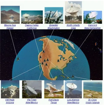
At present, one of the largest VLBI array is the Very Long Baseline Array (VLBA, Fig. 3.2), situated in USA, consisting of 10 identical radio antennas, each one with a diameter of 25 m, with baselines from ∼200 km (Los Alamos - Pie Town baseline, with both stations situated in New Mexico) up to∼8600 km (Mauna kea, Hawaii - St. Croix, Virgin Islands baseline). The VLBA operates in
Figure 3.2: Representation of the VLBA telescopes. Image courtesy of NRAO/AUI.
a frequency range from 1.2 GHz) to 86 GHz, reaching an angular resolution of the order of 0.12 milliarcsec at 86 GHz.
Othe major VLBI arrays are the European VLBI Network (EVN), with sta-tions in Europe, Asia, South Africa and Arecibo, and the Long Baseline Array (LBA) in the southern hemisphere.
To obtain an even higher angular resolution, a radio telescope in Earth orbit can be used, providing greatly extended baselines (Space VLBI). At present the Russian satellite RadioAstron is orbiting around Earth and together with some of the largest ground-based radio telescopes form baseline extending up to 350,000 km.
3.2. Towards the future: Square kilometer Array
Figure 3.3: Artist impression of the low-frequency sparse aperture array to be built in Australia (upper panel), of the mid-frequency (middle panel) and high-frequency (lower panel) arrays, to be built in Africa.
3.2
Towards the future: Square kilometer Array
The Square Kilometer Array (SKA) is a new generation revolutionary aperture synthesis radio telescope, that will combine signals from a network of antennas distributed over more than 3000 kilometers, producing a radio telescope with a collecting surface up to one square km and a very large field of view.
Ten countries (Australia, Canada, China, India, Italy, New Zealand, South Africa, Sweden, the Netherlands and the United Kingdom) are full members of the SKA international organization and around 100 organizations in about 20 coun-tries are collaborating for the scientific and technical development of the project.
The SKA will operate over a frequency range from 70 MHz up to 25 GHz, di-vided into three frequency bands: low-band from 70 to 300 MHz, mid-band from 0.3 to 10 GHz, and high-band from 10 to 25 GHz. The sensitivity improvement will be of about two orders of magnitude (reaching theµJy level) with respect to the current radio telescopes, and the expected survey speed improvement will be of about 4 orders of magnitude. A key feature of the SKA telescope is the capabil-ity to simultaneously observe multiple sky regions, by means of multiple indepen-dent beams, by increasing the telescope survey speed. The multi-beam capability will also increase the total field of view, which, at frequencies below 1 GHz, will reach several tens of square degrees. For all of these reasons, the SKA project will develop innovative technology for receiving systems, signal transport and computing. The SKA is a very ambitious and demanding project that will provide the development of new technologies, e.g. large field of view, multi-beam, high speed in data acquisition, computation, and a strong industrial return.
SKA will help astronomers to address numerous and fundamental astrophysi-cal questions such as the origin and evolution of the Universe, the formation and evolution of black holes, galaxies and large-scale structures, the origin of mag-netic fields and the nature of the dark energy. All of the main astrophysical topics investigated by SKA are represented by five key science projects: Galaxy
Evo-3.2. Towards the future: Square kilometer Array
lution, Cosmology and Dark Energy; Probing the Dark Ages; The Origin and Evolution of Cosmic Magnetism; Strong Field Tests of Gravity Using Pulsars and Black Holes; The Cradle of Life.
The two sites chosen for hosting SKA are the Western Australia’s Murchi-son Shire (hosting the low frequency array) and the South Africa’s Karoo region (hosting the mid and high frequency dishes), which, being among the most re-mote regions on Earth, are suitable for radio observations thanks to very low radio frequency interferences (RFI). The realization and the development of the SKA project is organized into two main phases, expected to be accomplished between 2018 and the late 2020s. For the phase 1, the low-frequency instrument, con-sisting of sparse aperture arrays with more than 500 stations, will be built in the Australian site (SKA1-low), while the mid-frequency instrument, possibly oper-ating at frequencies up to 20 GHz, will be built in the African site with an array of 200 dishes (SKA1-mid). With the phase 2 there will be the full realization of the telescope arrays in both sites, with one million of low frequency antennas and about 2000 high and mid frequency dishes. The design of the SKA low, mid and high-frequency arrays is shown in Fig. 3.3.
The VLBI capability of SKA can be implemented at the early stages with the SKA1-mid, by including it within the existing VLBI networks (SKA-VLBI). With a sensitivity down to µJy and an angular resolution down to the milliarcsecond, the SKA-VLBI will be an ideal tool, for example, for studying low luminosity AGNs and it will allow us to shed light on the details about the physics of the jet formation and the relation with the accretion processes. Thanks to the high-resolution SKA-VLBI polarimetric observations it will be possible to investigate the magnetic field structure close to the jet base, which is crucial for understanding the jet launch mechanisms and the related processes (Blandford & Payne 1982). Both as a stand-alone interferometer and as a VLBI sensitive element, SKA1 will have a fundamental impact on the study of AGNs in synergy with high energy observations (Agudo et al. 2015; Giroletti et al. 2015; Paragi et al. 2015).
Figure 3.4: Fermi satellite sketch, with the LAT (top yellow area) and the GLAST
(bot-tom) instruments.
3.3
The Fermi satellite
The Fermi Gamma-ray Space Telescope was launched on June 11, 2008 on an elliptical orbit at an altitude of about 565 km, with an inclination of 25.6◦ with respect to the Earth’s equator (Atwood et al. 2009). Fermi is the successor of the Energetic Gamma Ray Experiment Telescope (EGRET), on board the Compton Gamma Ray observatory (CGRO), which operated from 1991 to 2000 (Thompson et al. 1993). The Fermi satellite was intended and designed to mainly operate in survey mode. It covers the full orbit in about 96 min, and every ∼3 hours (two orbits) it scans the entire sky.
On board the Fermi satellite there are two scientific instruments: the Large Area Telescope (LAT) and the Gamma-ray Burst Monitor (GBM, Fig. 3.4). The LAT is the primary instrument. It is a pair conversion telescope which detectsγ rays in the energy range between∼20 MeV and ∼300 GeV, with a field of view of 2.4 sr, and an angular resolution1< 0.15◦for E >10 GeV (Atwood et al. 2009). As
illustrated in Fig. 3.5, the Fermi-LAT is made by a 4×4 array of towers, consisting of a tracker, in which γ rays are converted into charged pairs electron/positron, and a segmented calorimeter, which measures the electron-positron pairs energy.
1Single photon angular resolution (on-axis, 68% space angle containment radius) for