Alma Mater Studiorum - Universit`
a di Bologna
SCUOLA DI SCIENZE
Dipartimento di Fisica e Astronomia
Corso di Laurea in Astrofisica e Cosmologia
Kinematics modelling of molecular
gas in NGC 3100
Tesi di Laurea Magistrale
Presentata da: Francesco Fragnito Relatore: Chiar.mo Prof. Gabriele Giovannini Correlatore: Dott.ssa Isabella Prandoni Dott.ssa Rosita Paladino
Sessione I
This Thesis work was done as part of the research activity of
the Italian ALMA Regional Centre and of the Istituto di
Radioastronomia - Istituto Nazionale di Astrofisica (INAF) in
A Nicola e Filomena, insegnanti di professione e di vita.
Contents
Abstract 13
1 Introduction 15
1.1 Scientific Background . . . 15
1.1.1 AGN classification and radio galaxies . . . 16
1.1.2 AGN feedback and feeding . . . 20
1.2 The case of NGC 3100 . . . 23
1.2.1 The Southern radio galaxy sample . . . 23
1.2.2 NGC 3100 available information . . . 26
2 ALMA 28 2.1 Interferometers: principles and concepts . . . 28
2.1.1 Single-dish response . . . 29
2.1.2 Aperture synthesis . . . 30
2.1.3 Calibration: from observed to real visibilities . . . 33
2.1.4 Imaging process . . . 33
2.2 Observing with ALMA . . . 35
2.2.1 Front End, IF and Local Oscillator . . . 35
2.2.2 Back End and Correlators . . . 36
2.2.3 Water Vapour Radiometer . . . 36
2.2.4 Antennas and performance in Band 6 . . . 37
3 NGC 3100: ALMA Observations and Data reduction 39 3.1 Observations . . . 39
3.2 Inspection and data calibration . . . 40
3.2.1 CASA . . . 40
3.2.2 Data import, inspection and flagging . . . 41
3.2.3 A priori calibration . . . 41
3.2.4 Data calibration . . . 43
3.2.5 Data examination . . . 45
3.3.1 Continuum image . . . 47
3.3.2 CO line Image . . . 49
4 NGC 3100: Data Analysis 51 4.1 CO line Moment Maps . . . 51
4.2 The CO as molecular gas tracer . . . 53
4.3 Comparison with dust and radio continuum . . . 55
5 Kinematics modelling of the CO disk 59 5.1 Tilted-ring model . . . 59
5.1.1 Fitting algorithms: an overview . . . 63
5.2 NGC 3100 models . . . 65
5.2.1 Model assumptions . . . 65
5.2.2 TiRiFiC models . . . 69
5.2.3 3D-Barolo models . . . 74
5.2.4 Moment 1 maps of the models . . . 87
Conclusions 90
List of Figures
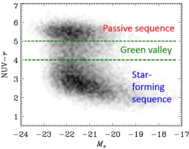
1.1 Bimodality in the color distribution of local galaxies. . . 16
1.2 The unification model for AGNs. . . 18
1.3 Bondi accretion power versus the jet power. . . 22
1.4 CO(2-1) APEX spectra for eight radio galaxies of the Southern Sample. . . 25
1.5 Observations of NGC 3100. . . 27
2.1 Normalized 1-D antenna power response for a 12-m antenna . 29 2.2 Normalized 1-D antenna power response for a 12-m antenna . 31 2.3 uv-plane coverage for NGC3100 observation. . . 32
2.4 Atmospheric transmission PWV. . . 35
2.5 Schematic view of ALMA LO and IF system. . . 36
2.6 Band 6 zenith transmission for PWV. . . 37
2.7 Typical Tsys at zenith for Band 6. . . 38
3.1 Antennas configuration. . . 40
3.2 WVR corrections. . . 42
3.3 Tsys table corrections. . . 43
3.4 Model calibrator. . . 44
3.5 Solutions for amplitude and phase as a function of time. . . . 45
3.6 Corrected visibilities of J1037-2934 and NGC3100. . . 45
3.7 Corrected visibilities of J1037-2934. . . 46
3.8 CO(2-1) double-horned line of NGC 3100. . . 47
3.9 NGC 3100 continuum image. . . 48
3.10 NGC3100 continuum image self-calibrated. . . 49
3.11 NGC3100 CO(2-1) line channel map. . . 50
4.1 Integrated intensity map (moment 0). . . 52
4.2 Integrated velocity map (moment 1). . . 53
4.3 ALMA moment 0 map and continuum. . . 54
4.4 Moment 0 map over the B-I HST dust image. . . 56
4.6 Continuum image of ALMA and VLA. . . 58
5.1 The bending model. . . 60
5.2 The orientational parametrization of 3D-Barolo. . . 61
5.3 TiRiFiC and 3D-Barolo model construction and fitting . . . . 64
5.4 Inclination of the model. . . 67
5.5 Velocity field of a rotating disk with additional non-circular motion. . . 68
5.6 Moments 1 of NGC 3100 created by Barolo. . . 68
5.7 TiRiFiC rotational model. . . 70
5.8 TiRiFiC non-circular model. . . 71
5.9 TiRiFiC rotational model channel maps. . . 72
5.10 TiRiFiC non-circular model channel maps. . . 73
5.11 TiRiFiC models PV diagrams. . . 74
5.12 3D-Barolo rotational model parameters. . . 76
5.13 3D-Barolo non-circular model parameters. . . 77
5.14 Surface brightness produced by Barolo. . . 77
5.15 3D-Barolo rotational model channel maps. . . 78
5.16 3D-Barolo local non-circular model channel maps. . . 79
5.17 3D-Barolo azimuthal non-circular model channel maps. . . 80
5.18 3D-Barolo local non-circular model channel maps. . . 81
5.19 3D-Barolo azimuthal rotational model PV diagrams. . . 83
5.20 3D-Barolo local rotational model PV diagrams. . . 84
5.21 3D-Barolo azimuthal non-circular model PV diagrams. . . 85
5.22 3D-Barolo azimuthal non-circular model PV diagrams. . . 86
5.23 Moments 1 of TiRiFiC models. . . 87
5.24 Moments 1 of azimuthal 3D-Barolo models. . . 88
5.25 Moments 1 of local 3D-Barolo models. . . 88
List of Tables
1.1 General properties of the Southern Sample radio galaxies. . . . 24 1.2 APEX-1 CO(2-1) line measurements of the Southern Sample. . 26
Sommario
Questa tesi `e parte di un progetto cha ha come obiettivo effettuare uno studio completo di differenti componenti galattiche (stelle, gas freddo e caldo) nei nuclei di galassie radio-loud di tipo early-type e ricercare segni cinematici di feeding/feedback che possano essere associati in modo causale alla presenza di getti radio. Per questo scopo `e stato selezionato un campione di undici galassie a z < 0.03 dalla survey Parkes 2.7-GHz, osservate tramite spettro-scopia ottica dal VLT/VIMOS (per la componente stellare e di gas caldo) e dall’interferometro ALMA (per la componente di gas molecolare). In parti-colare, la tesi `e incentrata sulla cinematica del gas molecolare nel centro di una delle sorgenti del campione: NGC 3100, una radiogalassia di tipo FRI ospite di una galassia lenticolare a redshift z = 0.0088.
NGC 3100, da osservazioni effettuate dal radiotelescopio APEX a 230 GHz, mostra una riga spettrale del CO(2-1) a doppio corno consistente con la presenza di un disco in rotazione (Laing et al. in prep). La regione pi`u interna di NGC 3100 `e stata quindi osservata nella Banda 6 di ALMA durante il Ciclo 3.
Come parte di questa tesi, i dati ALMA sono stati ridotti ed `e stato ottenuto un data cube con un beam di 0.73 arcsec2 dove `e chiaramente de-tettata una riga del CO(2-1) a 230 GHz, che mostra una struttura rotante a forma di anello.
Inoltre, analizzando i dati del continuo di ALMA si possono osservare le regioni pi`u interne dei getti radio della galassia, che sono perfettamente consistenti con le osservazioni effettuate con VLA a 5 GHz e 8.5 GHz con una simile risoluzione spaziale. Un’analisi completa dell’emissione in riga del CO(2-1) `e stata effettuata attraverso una mappa d’intensit`a integrata (momento 0 ) ed una mappa di velocit`a integrata (momento 1 ). E stata` quindi trovata una massa di gas molecolare pari a M = 1.85 ± 0.4 × 10⁸M
, consistente con ci`o che si `e trovato con APEX. La mappa del CO `e stata quindi confrontata con la distribuzione della polvere (da un’immagine B-I in assorbimento) nelle regioni pi`u interne della galassia ospite. Ci`o ha portato ad una soddisfacente sovrapposizione tra le strutture detettate in entrambe
le immagini.
Il disco di gas molecolare mostra una cinematica complessa, con alcuni warp nel campo di velocit`a.
`
E stata quindi effettuata una modellizzazione del disco attraverso due software: TiRiFiC e 3D-Barolo. Un confronto tra i risultati dei due pro-grammi `e risultato utile per comprendere la cinematica del gas. La modelliz-zazione ha infatti confermato le assunzioni iniziali circa l’inclinazione (∼ 60◦) e il position angle (∼ 230◦) del disco. Ci`o ha permesso di produrre e con-frontare, infine, campi di velocit`a puramente rotazionali e campi di velocit`a con moti non circolari.
Abstract
This thesis is part of a project aimed at providing a comprehensive study of different galaxy components (stars, warm, cold gas) in the core of radio-loud early-type galaxies, and look for kinematical signatures of feeding/feedback loops that can be causally related to the presence of radio jets. For this purpose a complete, volume limited (z < 0.03) sample of eleven radio galaxies in the Southern sky was selected from the Parkes 2.7-GHz survey. This sample is the target of VLT/VIMOS integral-field-unit optical spectroscopy (warm gas and stellar components) and ALMA CO line imaging (molecular gas). This thesis inquires into the kinematics of molecular gas in the centre of one of the sources in the sample: NGC 3100, a FRI radio galaxy hosted by a S0 galaxy at redshift z = 0.0088.
NGC 3100 was observed with APEX at 230 GHz and showed a CO(2-1) line profile (double-horned) consistent with the presence of a rotating disk (Laing et al. in prep). The inner region of NGC 3100 was then imaged with ALMA at Band 6 during Cycle 3.
As part of this thesis, ALMA data was reduced and a data cube was obtained with a beam of 0.73 arcsec2, where a CO(2-1) 230-GHz line was clearly detected. The line is organized in a ring-like rotating structure.
The ALMA radio continuum data, on the other hand, revealed the inner part of the radio jets, entirely consistent with those imaged at similar reso-lution with the VLA at 5 GHz and 8.5 GHz. A full analysis of the CO(2-1) line emission was made through the integrated intensity map (moment 0 ) and the integrated velocity map (moment 1). The mass of the molecular gas resulted in M = 1.85 ± 0.4 × 10⁸M
, consistent with what found with APEX. The CO map was compared with the distribution of dust (from B-I absorption image) in the inner region of the host galaxy. A nice overlap was found for the structures detected in both images.
The molecular gas disk shows a complex kinematics, with some warps in the velocity field.
Two programs were used to model the disk: TiRiFiC and 3D-Barolo. The comparison of their results was helpful to better understand the kinematics
of the gas. The modelling confirmed initial guesses about the inclination (∼ 60◦) and the position angle (∼ 230◦) of the gas disk, and allowed us to derive purely rotational velocity fields as well as fields including non-circular motions.
The thesis is organized in five Chapters:
• In the first Chapter the scientific background is briefly presented as well as the Radio Galaxy NGC 3100.
• In the second Chapter an introduction to radio interferometry and the ALMA telescope is given.
• The third Chapter is focused on the ALMA data reduction of NGC 3100 continuum and CO(2-1) 230-GHz line emission.
• In the fourth Chapter the analysis of the ALMA data is presented, together with a comparison with radio continuum (VLA) and dust absorption images.
• In the fifth Chapter the TiRiFiC and 3D-Barolo modelling programs are presented and their results are discussed.
Chapter 1
Introduction
1.1
Scientific Background
Large-scale properties and scaling relations of early-type galaxies (ETGs) that compare surface brightness, velocity dispersion and stellar mass (e.g. Faber-Jackson, M − σ relation) provide important information in order to trace the fossils of galaxy formation processes, as ETGs are old evolved galax-ies, that generally present limited star formation and dust content.
The Sloan Digital Sky Survey (SDSS; York et al. 2000) has given a significant contribution in the understanding of formation of local ETGs, based on the statistically significant bimodality in the galaxy colour distri-bution. Local galaxies can be separated in two distinct groups: the so-called “blue cloud”, mainly constituted by star-forming disk galaxies, and the “red sequence”, constituted by massive and passive ETGs; a minor fraction of galaxies can be found in the so-called “green valley”. This bimodality has been interpreted as the result of galaxy evolution. Galaxies grow with time due to ongoing star formation and move toward the high-mass end of the blue cloud and then rapidly move to the red sequence (Figure 1.1). A mechanism that efficiently suppresses episodes of intense star formation and expels gas from the system is needed in order to allow this rapid transition (e.g. Faber et al. 2007). Several mechanisms have been invoked: active galactic nucleus (AGN) feedback (in the form of quasar winds), supernovae winds, gravita-tional gas heating or shock heating in massive halos.
On the other hand, dissipationless dry mergers of red sequence galaxies are thought to be responsible for the formation of the most massive ETGs (e.g. Oser et al. 2010), while heating from radio jets (jet-induced feedback) is thought to be responsible for suppressing star-formation in ETGs, and mantaining them on the red sequence (i.e. “red and dead”). Indeed, ETGs
host a wide range of kinematically decoupled components, central stellar disks, and other peculiarities (e.g. Emsellem et al. 2004). The suppression of star formation in ETGs and the formation of sub-structures may well be connected and both related to AGN feedback and fueling cycles.
Figure 1.1: UV-optical color magnitude diagram showing the bimodality in the color distribution of local galaxies between star-forming galaxies (blue cloud) and passive galaxies (red sequence) with the transitional green valley. Data from the z < 0.22 GALEX/SDSS sample (Salim et al. 2007).
A comprehensive study of the various gas phases, as well as the stellar and dust components in a representative sample of massive, radio-loud ETGs (in which jets are currently active) could provide a crucial comparison to existing studies of radio-quiet ETG samples (e.g. AT LAS3D; Cappellari et al. 2011; Young et al. 2011; Alatalo et al. 2013; Davis et al. 2011, 2013a). It will enable a better understanding of the feeding of AGNs, and will isolate the role played by jet-induced feedback (likely dominant in local, massive ETGs) in the overall formation and evolution of ETGs.
Throughout this work distances and luminosity have been computed as-suming a CDM cosmology, where:H0 = 70kms−1M pc−1, ΩM = 0.3 and Ωλ = 0.7.
1.1.1
AGN classification and radio galaxies
The term Active Galactic Nucleus (AGN) generally indicates an extremely energetic phenomenon in the nucleus, or in the central region, of a galaxy.
The basic structure of an AGN is composed by:
• A central black hole (BH) with mass ranging from 106M
up to109−10M , probably spinning at some level.
• An accretion disk formed by matter attracted by the gravitational po-tential of the BH.
• A corona sorrounding the accretion disk and particularly active in emit-ting X-ray light.
• A region filled by small clouds distant less than one parsec from the BH. This is the so-called Broad Line Region (BLR). It absorbs ∼ 10% of the radiation from the disk and re-emits it in the form of emission lines with typical velocity dispersions of ∼ 3000kms−1.
• An obscuring torus located at several parsec from the BH, that re-processes part of the nuclear radiation and re-emits it in the infrared band.
• A more distant region (∼ 100pc) where less densely diffuse clouds are moving with characteristic velocities of ∼ 300 − 500kms−1 named Nar-row Line Region (NLR).
Figure 1.2: The unification model for AGNs. Blazars are RL AGNs for which the jets are close to LoS. They are divided in BL Lacertae objects (BL Lac) and Flat Spectrum Radio Quasar (FSRQ). If the orientation angle is ∼ 30o (both NLR and BLR are visible), a RQ quasar (QSO), a Steep Spectrum Radio QSO (SSRQ) or a Seyfert 1 galaxy is observed. At larger angular offsets, the BLR is hidden by the torus, and we observe Narrow Line Radio Galaxies (NLRG) or Seyfert 2 galaxies. Perpendicular to the jet axis, the full extent of the jets (when present) can be seen.
The emission lines coming from the BLR are usually originated by permit-ted transitions, the most relevant belonging to Balmer and Lyman Hydrogen series. The NLR emits both forbidden and permitted lines, the most evident among the former being the lines produced by ionized Oxygen and Neon.
A basic classification scheme divides AGN in loud (RL) and radio-quiet (RQ) depending on their radio properties. Radio-loud AGNs show two collimated jets of plasma feeding extended lobes or a halo, both emitting in the radio continuum. Radio-quiet AGNs show weak or no large scale jets.
According to the Unification Model (Antonucci, 1993; Urry & Padovani, 1995) the observed AGN properties depend on the inclination of the system with respect to the line of sight (LoS) to the observer. When the observing angle is large, the torus hides the emission from the inner parts of the system
including the BLR. Only the NLR is visible and the object is classified as a Type 2 AGN. When the AGN is viewed at intermediate inclination the inner regions becomes visible together with the NLR, and the AGN is classified as a Type 1 object. RL AGNs whose jets point toward us are called Blazars; when the jets point elsewhere they are called Radio Galaxies (RG). A schematic representation of the classification is shown in Figure 1.2, where different terminology is used depending on whether the AGN is RL or RQ.
Radio Galaxies typically show the following components:
• Radio Lobes, extended structures with almost elliptical shape and sym-metrical locations with respect to the central object. The distance of the lobes spans from few tens of kpc up to 1 Mpc and their luminosity usually decreases going from the edges to the centre.
• Hot Spots, regions with little extension and higher luminosity compared with the lobes. The hot spots usually marks the end point of a well collimated jet for a high power radio galaxy.
• Core, central compact component that usually gives little contribution to the overall radio emission. Its contribution is typically larger in low power radio galaxies.
• Jets, elongated and narrow structures typically starting from the core. Their end is marked by the hot spots where the material, expelled from the core and funnelled by the jets, hits the surrounding medium. The appearance of the jets depends on their radiative efficiency. A well collimated jet does not show large radiative losses, and virtually all the energy is channelled toward the hot spot, while a radiative efficient jet loses a large amount of its energy on its way and is generally associated to weak or no hot spot.
Fanaroff & Riley (1974) divided the radio galaxies in two classes, known with the names of FRI and FRII, looking at the morphology of the large-scale radio emission. FRI sources appear brighter toward the centre (edge-darkened), while FRII are brighter at the edges (edge-brightened). Further-more, they noted that the two classes are characterized by different luminosi-ties. Sources with luminosity Lradio ≤ 2 × 1025W Hz−1sr−1are often (but not always) FRI, while brighter sources are often FRII. The two morphological types clearly show different behaviour in their optical spectra (Laing et al. 1994, Buttiglione et al. 2010). The FRI radio galaxies hosts typically exhibit optical spectra with absorption lines and/or low ratios of O[III]/Hα < 0.2
. Following the classification of Laing et al. (1994) these galaxies are clas-sified as Low Ionization Emission Line Radio Galaxies (LERGs). On the other hand, FRII host galaxies appear as a mixed class: they can show ei-ther FRI-like spectra or strong high ionization emission lines characterized by O[III]/Hα > 0.2 (High Ionization Emission line Radio Galaxies, HERGs).
Observational evidence is growing that LERGs constitute a different type of AGNs that does not fit into the unification model and a distinct mode of accretion onto the supermassive black hole (SMBH) exists (advection-dominated, ADAFs, or radiatively inefficient accretion flows, RIAFs). These types of AGN are often capable of launching two-sided jets and lack a dust torus. The geometrically-thin accretion disk is either absent, or is truncated in the inner regions and it is replaced by a geometrically-thick structure in which the inflow time is much shorter than the radiative cooling time (Heckman & Best, 2014).
1.1.2
AGN feedback and feeding
SMBHs are thought to play a principal role in regulating star formation in galaxies across cosmic time. The process by which this occurs is known as AGN feedback and it takes place through an interaction between the energy and radiation released by black hole accretion and the gas in the host galaxy. Two major modes are identified, differentiated by the nature of the en-ergy outflow near the black hole. The first is the so-called radiative mode. This feedback takes the form of quasar-driven winds that expel gas from the galaxy centre. It is typically associated with black hole accreting close to the Eddington limit. The second mode is the so-called kinetic mode, also known as jet mode. In this case the energy is released in form of collimated jets that wipe out the intra-galactic medium on their way and heat the surrounding gas. It tends to occur in massive galaxies embedded in hot gas halos (Fabian 2012). In particular, radio-emitting jets are common in massive elliptical galaxies at the centre of galaxy clusters and lead to the formation of cavities in the intergalactic medium (IGM) surrounding them. The radio jets are thought to heat the gas in the so-called cool-core clusters, preventing further cooling and thereby suppressing star formation. This should also prevent further fueling of the BH and eventually lead to the switch off of the radio jets. However, many details are missing and the mechanisms by which jetted AGN are fuelled and the way in which this forms part of a feedback loop are not yet fully understood.
Two principal accretion modes are invoked for the AGN feeding: the cold accretion (accretion of cold circumnuclear gas) or accretion from hot keV
atmosphere (Bondi accretion). We have seen that RGs can be divided in the two classes of HERGs and LERGs. These two classes are characterized by different accretion rate onto the central SMBH. The first class, radiative mode AGN, accrete at ≥ 1% of the Eddington limit. In the second class, jet mode AGN, the accretion rate and the radiative output from the AGN are both much lower (Heckman & Best, 2014).
Allen et al. (2006) have found that the rate of accretion of the X-ray emitting gas at the accretion radius (the radius within which the gravitational potential of the central black hole dominates over the thermal energy of the surrounding X-ray emitting gas) can be written as (Bondi, 1952):
˙
MBondi = 4πλ(GMBH)2csρ
where ρ is the density of the gas at the accretion radius, MBH is the central black hole mass, G is the gravitational constant, cs is the adiabatic sound speed of the gas at the accretion radius and λ is a numerical coefficient that depends upon the adiabatic index of the accreting gas. For an efficiency η, the maximum power released from the black hole system is
PBondi = η ˙MBondic2.
They found a correlation between the Bondi accretion rate and jet power for LERGs and proposed that accretion in these systems may occur directly from the hot phase of the IGM (Figure 1.3). Indeed, the kinetic power of the jets was computed through the estimates of the energy E required to create observed cavities in the X-ray emitting gas by the jets and the life time of these cavities tage:
Pjet = E tage
.
Subsequently, Hardcastle et al. (2007) confirmed that the energy required to power non-thermal emission from LERGs could be provided by Bondi accretion. This is not the case for HERGs where an extra component is needed to sustain the observed jet powers. The most plausible candidate for this extra-component is cold gas brought to the center through mergers (cold accretion).
Figure 1.3: The logarithm of the Bondi accretion power versus the logarithm of the jet power. Both the quantities are in units of 1043erg s−1. The dashed lines shows the bestfitting linear-plus-constant model.
Even though enough energy can be provided by accretion of hot gas at the Bondi rate, this does not prove that LERGs are powered in this way. The reason is that the mass of material actually reaching the black hole may be significantly lower than the Bondi estimate, as spherical symmetry must break down at some radius.
Russel et al. (2013) re-examined the relationship between the jet power and the Bondi accretion rate. The results indicate weaker evidence for a correlation between Bondi accretion and jet power. He suggested that cold gas fuelling could be a likely source of accretion power in these objects, even if he could not rule out Bondi accretion, which could play a significant role in low-power jets.
This gas may cool from the hot phase, as in the ‘cold feedback’ or ‘chaotic cold accretion’ models (Pizzolato & Soker, 2005; Gaspari et al., 2013), but could also come from stellar mass loss, interactions or mergers. Some support for the idea that at least the most powerful LERGs are fuelled by accretion of cold gas comes from the direct detection of dust and cold molecular gas in these systems (de Ruiter et al., 2002; Lim et al., 2003; Leon et al., 2003; Prandoni et al., 2007, 2010; Oca˜na Flaquer et al., 2010). But the presence of large masses of molecular gas is not direct evidence of fuelling. Dust in radio galaxies is often localised in well-defined disks on small scales (≤ 2.5 kpc). Similarly, the observed CO line profiles often show the double-horned pro-files characteristic of rotating disks. Very few high-resolution images of CO emission are available, but Okuda et al. (2005) made interferometric obser-vations of the radio galaxy 3C 31 and showed that the CO, which coincides spatially with the dust disk observed in HST images, is in ordered rotation. If the cold gas is in stable orbits, as suggested by Okuda et al. (2005), then the accretion rate may be relatively low. In other galaxies, the molecular gas appears to be outflowing (or more generally interacting with) the radio jets or lobes. The incidence of these different types of molecular gas distribution in typical radio galaxies (as opposed to extreme cases) is not known. The key instrument for such an analysis is ALMA. However, very little is currently known about cold gas in the southern radio galaxies that can be observed at high elevation with ALMA. For this reason a complete volume-limited sample of radio galaxies in the Southern hemisphere has been selected for systematic CO observations.
1.2
The case of NGC 3100
1.2.1
The Southern radio galaxy sample
The Southern radio galaxies sample was selected from the Parkes 2.7-GHz survey. This survey collects 191 RGs located in the declination range −17o < δ ≤ 40o with a radio flux-density limit of 0.25 Jy at 2.7 GHz and an optical magnitude limit of mV ≤ 17.0 (Ekers et al. 1989). The two selection criteria applied to select the Southern radio galaxies sample were:
• association of the source with an Elliptical or S0 galaxy • host galaxy redshift z < 0.03
The eleven selected sources have all low or intermediate radio powers and a FRI radio morphology.
Table 1.1: General properties of the Southern Sample radio galaxies. From col. 1 to col. 3: radio source name, host galaxy name and redshift. In col. 4 and 5: the radio flux density at 1.4GHz and corresponding radio power. In col. 6, the FR type. In col. 7 and 8: the apparent and absolute magnitudes in K band. Then, in order of columns: velocity dispersion, optical dust morphology, dust temperature and mass from IRAS obsevations. The optical dust information come from: (a) Bettoni et al. (2001); (b) Lauer et al.(2005); (c) Colbert et al. (2001); (d) Sandage & Brucato (1979), (e) Govoni et al. (2000).
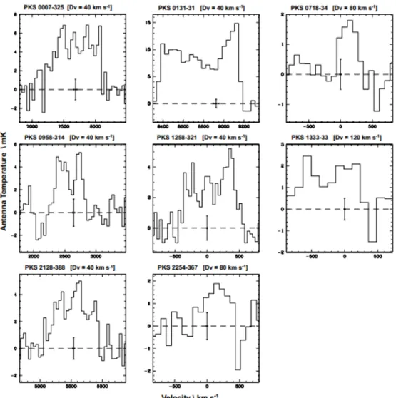
The main characteristics of the Southern Sample galaxies are listed in Table 1.1. Emission in the CO(2-1) transition at 230 GHz rest frequency was investigated for ten of the eleven sources with the APEX single dish telescope (Prandoni et al. 2010; Laing et al. in prep). The 27 arcsec APEX Half Power Beam Width probes the presence of molecular gas in the inner 2.7-16.2 kpc of the host galaxies (depending on redshift). This allows a direct comparison with the dust structures on similar scales imaged with HST, when available (Lauer et al. 2005). All sources were detected at either 40 or 80 km−1 velocity resolution. In Figure 1.4 are shown eight CO(2-1) APEX spectra (of the ten obtained) discussed in Laing et al. (in prep.).
Figure 1.4: CO(2-1) APEX spectra for eight radio galaxies of the Southern Sample. Dv is the velocity channel width. The vertical and horizontal er-ror bars at the systemic velocity (Vsys) indicate the RMS on the Antenna
Table 1.2: APEX-1 CO(2-1) line measurements of the Southern Sample. (a ) Sources studied by Prandoni et al. (2010), (b ) Source studied by Horellou et al (2001)
For the majority of the sources the CO lines show double horn or flat pro-files, consistent with ordered rotation. The Southern Sample RGs typically show large linewidths (≥ 500kms−1), and the derived molecular masses span a range between 107−9M (see Table 1.2).
1.2.2
NGC 3100 available information
Nine of these radio galaxies were followed up with ALMA during cycle 3. In this thesis I present the ALMA data analysis for one of them: NGC 3100 (RA(J 2000) = 10 : 00 : 40.8; DEC(J 2000) = −31 : 39 : 52).
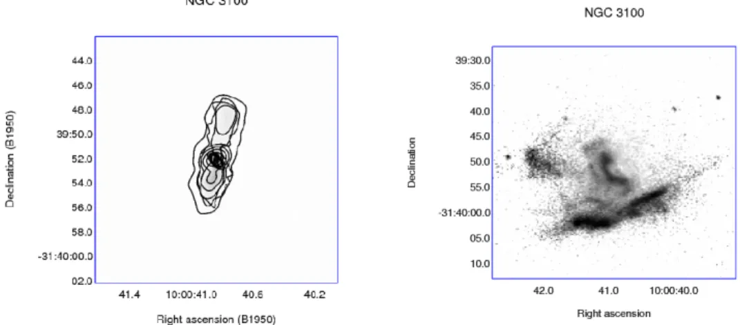
NGC 3100 is FRI radio galaxy (left panel of Figure 1.5) hosted by a S0 galaxy at redshift z = 0.0088 corresponding to a luminosity distance DL= 40.9 M pc.
Figure 1.4 shows that NGC 3100 (PKS 0958-314) is characterized by a double-horn CO profile on a scale of (at least) ∼ 5 kpc (see Table 1.2), consistent with the presence of a rotating disk. In addition NGC 3100 shows a patchy dust morphology (right panel of Figure 1.5).
Figure 1.5: Observations of NGC 3100. Left : 5 and 8.5 GHz VLA radio continuum image showing a twin radio jet. Right: NGC 3100 optical B-I image showing the central diffuse dust.
NGC 3100 can be spectroscopically classified by using the standard [OIII]λ5007/Hβ versus [N II]λ6583/Hα BPT diagnostic diagram (Baldwin, Phillips and Terlevich 1981) and its following revisions (Kewley et al. 2001, Kauffmann et al. 2003, Kewley et al. 2006). In such a diagram galaxies which are likely to be dominated by an AGN can be separated from galaxies dominated by star formation. In addition Seyfert galaxies can be distin-guished from Low Ionization Nuclear Emission Regions (LINER) galaxies. In this manner, Dopita et al. (2015) identifies NGC 3100 as a LINER with very low extinction, but with deep NaD absorption. As such, NGC 3100 belongs to the LERG class.
Chapter 2
ALMA
The Atacama Large Millimeter/submillimeter Array (ALMA) is an aperture synthesis array operating in the millimeter and submillimeter regime. It is located on the Chajnantor plain of the Chilean Andes, 5000 m above sea level, where the site offers the best weather conditions required to observe in (sub)mm wave range.
In September 2011, the telescope started its Early Science period with a reduced number of antennas, frequency bands, array configurations and observing modes. ALMA consists of two principal arrays:
• 12-m Array, composed by fifty 12-meter antennas, that can be arranged in different configurations with baselines from 15 m up to 16 km.
• Atacama Compact Array (ACA), composed by twelve 7-m antennas (with 9 to 30 m baselines) plus four 12-m single-dishes, designed to solve the so-called zero-spacing problem (See Section 2.1.2).
The ALMA observations used for this thesis have been taken during Cycle 3, with the 12-m array. The basics of Interferometry and the main charac-teristics of ALMA will be illustrated in this Chapter.
2.1
Interferometers: principles and concepts
Interferometry is an observational technique used in millimeter/radio and visual regime, based on the principle of interference of incoming electro-magnetic waves. It involves coherent arrangement of sky signals received by separated antennas pointed to the same object. The signals are interfered, al-lowing the sampling of sky brightness distribution on an angular scale smaller than what is possible with the single antennas composing the array.
2.1.1
Single-dish response
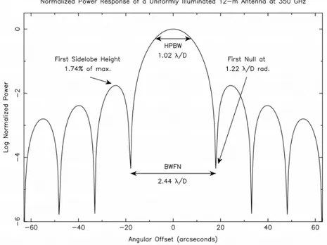
According to the Fraunhofer diffraction theory, it is possible to consider the electromagnetic (EM) power of wavelength λ from a point-like source at infinity arriving at an antenna of diameter D essentially as plane-parallel wavefronts along its axis. The diffraction pattern in the aperture of an an-tenna is related to the power distribution through a Fourier transform. This results into the so-called power pattern, or beam. It represents the response in the focal plane of the antenna to EM signal (Figure 2.1).
The on-axis central Gaussian-like feature is called primary beam or main-lobe and it has a Half Power Beam Width (HPBW) of ∼ λ/D, where λ is the wavelength of the incident wave and D is the diameter of the antenna. Sidelobes at off-axis angles may be identified. They are related to summed EM interference, decreasing with increasing angular off-set. The distance between nulls is defined Beam Width at First Nulls (BWFN) with a value of 2.44λ/D. Half the BWFN of the primary beam, 1.22λ/D, is the Rayleigh resolution of the antenna, the minimum angular distance between two objects for which they can be seen as separated. The beam is affected by various effects that may corrupt the measured power, such as surface imperfections or diffraction from other antenna components.
Figure 2.1: Normalized 1-D antenna power response for a 12-m antenna uni-formly illuminated at 300 GHz. The power is in log units to emphasize the sidelobes. HPBW measured from actual 12-m ALMA antennas is ∼ 1.13λ/D.
The actual ALMA antennas were constructed to provide the best response with a nearly gaussian primary beam and low sidelobes with HPBW values of ∼ 1.13λ/D for the 12-m antennas. This value is the so-called Field of View (FoV):
F oV ∼ 1.13λ/D [radians] The total power received by each antenna is defined as:
Prec = 1 2Ae Z 4π Iv(θ, φ)PN(θ, φ) dΩ
where Ae is the effective area of the antenna, θ and φ are the sky coor-dinates, Iv(θ, φ) the directional function of the sky brightness distribution and PN(θ, φ) the normalized antenna power pattern. The value 1/2 is due to to the fact that the receiver is generally sensitive to only one mode of polarization.
The effective area of antennas differs from their geometric area (π(D/2)2) by a factor ηA= Ae Ageom ≤ 1
2.1.2
Aperture synthesis
As shown, the resolution of a single-dish observation increases with λ, and decreases with the diameter D of the antenna. In particular, radio/(sub)mm observations have typically poor resolution, as the value of λ is much larger (compared to optical observations) while the maximum antenna diameter D is limited by technique.
For this reason, interferometry, or aperture synthesis, is used to improve angular resolution of the system. An interferometer is composed by two or more antennas, whose signals are combined.
Each pair of elements is spaced by a distance b called baseline (Figure 2.2). The power response of the antennas of a pair is time-averaged and cross-correlated by the correlator. The multiplication of the voltage patterns from element pairs is the resulting power pattern of the interferometer.
Figure 2.2: Interferometer consisting of two antennas, spaced by a physical distance b. The antennas are both pointed towards a sky location s0, distant
θ from the meridian.
As two antennas observe the same object with a delay given by τ = bs0/c, where s0 is the position observed by the antennas and c is the light-speed, it is applied an artificial delay to the signal received by the first antenna before correlating the signals. At this point, the correlator multiplies and time-averages the signals coming from the two receivers and measures the so-called quantity complex visibility, V (x, y).
The complex visibility is the Fourier transform of the sky brightness dis-tribution B(x, y) (Cittert-Zernike theorem):
V (u, v) =
Z Z
B(x, y)e2πi(ux+vy)dxdy = V0eiφ
B(x, y) =
Z Z
V (u, v)e−2πi(ux+vy) dudv
where u and v components (in λ units) are the projection of each baseline onto the observed sky-plane in E-W and N-S directions, the x and y spatial components (in radians) are the position in the sky plane. The visibility V gives information about source brightness and phase centre through its amplitude V0 and its phase φ.
Figure 2.3: uv-plane coverage for the NGC3100 Cycle 3 ALMA observation. The integration time is 44min; u and v are in meter unit.
The uv-plane as visibility distribution gives information about sky bright-ness distribution on the sampled angular scales.
The sky sampling carried out from a pair results in a brightness distribu-tion on a scale inversely propordistribu-tional to its length (∼ λ/b for the 1-D case). The short baselines sample larger scale and the longer ones sample shorter scale. Observing shorter or longer wavelengths sample smaller or larger an-gular scales, respectively. Different antennas pairs allow to sample different scales, corresponding to different points in the uv-plane (Figure 2.3). The baselines projection plane is affected by the Earth’s rotation that changes the position of the uv points, allowing to sample more scales.
Interferometer properties
As seen for the single-dish, the FoV in aperture synthesis represents the angular sensitivity pattern on the sky of each element in the array. In this case it is also named primary beam keeping the same physical definition
F oV ∼ 1.13λ/D [radians]
The angular resolution of an interferometer, called synthesized beam, can be written as:
θres= k λ Bmax
where k is related to visibilities weighting and Bmax is the longest baseline in the array.
Baselines shorter than the diameter of an antenna are impossible to be produced. This introduces the so-called zero-spacing problem: regions of the uv-plane related to distances closer than the minimum baseline cannot be sampled. For this reason, there is a maximum angular scale structure that an interferometer recovers, the Maximum Recoverable Scale (MRS):
θM RS ≈ 0.6 λ Bmin
[radians]
where Bmin is the minimum baseline of the array configuration.
2.1.3
Calibration: from observed to real visibilities
Instrumental and atmospheric effects corrupt the visibilities obtained with an interferometer. For this reason, calibration is needed to correct such effects and to recover the real visibilities from the observed ones.
The Hamaker-Bregman-Sault Measurement equation expresses the rela-tionship between observed and real visibilities for a baseline between antenna i and j :
Vijobs(ν, t) = GijVijreal(ν, t) + noise where Vobs
ij represents the observed visibilities, Vijreal represents the corre-sponding real ones and Gij are the gain factors and represent the combination of all the corruption factors related to the baseline ij.
The gain factors can be decomposed into time-dependent and frequency-dependent components, which are assumed to be infrequency-dependent from each other:
G = B(ν)J (t)
where B(ν) represents the frequency-dependent components and J (t) repre-sents the time-dependent components.
The measurement equation is solved by observing one or more calibrator sources with known properties to determine the different gain factor. Once solutions are found, the gain factors are stored in calibration tables and applied to the observed visibilities of the science target (See Section 3.2.4).
2.1.4
Imaging process
The observed visibilities of a target are ideal visibilities sampled only in discrete points of the uv-plane. This can be expressed as:
where V (u, v)meas are the observed visibilities,V (u, v)true are the ideal visi-bilities and S(u, v) is the so-called sampling function, an 1-result indicator function (S(u, v) = 1 where data are taken, S(u, v) = 0 where no data are available).
The measured sky brightness distribution is obtained by computing the inverse Fourier transform of (1), achieving the so-called dirty image:
Imeas = F T−1(Vmeas) = F T−1(S) ⊗ F T−1(Vtrue)
where Imeas is the measured sky brightness distribution, and the inverse Fourier transform of the sampling function is called dirty beam.
The incomplete spatial frequency sampling produces aliased features in the resulting image. The CLEAN algorithm is an iterative method which makes a deconvolution of the dirty image from the dirty beam to minimize these effects. It proceeds as follows (considering Hogbom algorithm):
• Initializes the residual map to the dirty map, and the Clean component list to an empty value;
• Identifies the pixel with the peak of intensity (Imax) in the residual map, and adds to the clean component list a fraction of Imax = γImax, (γ ∼ 0.1, 0.3);
• Multiplies the clean component by the dirty beam and subtract it to the residual map;
• Iterates until stopping criteria are reached: |Imax| < multiple of the rms (when rms limited); |Imax| < fraction of the brightest source flux (when dynamic range limited);
• Multiplies the clean components by the clean beam, which is an ellip-tical Gaussian fitting of the central region of the dirty beam, and add it back to the residual (restore).
During the imaging process it is possible to modify the weight of the visi-bilities considering the weighting function W(u,v). It permit to change image resolution and sensitivity. The true density distribution of the visibilities in the uv-plane is given by natural weighting (W (u, v) = 1/σ2(u, v), where σ is the noise variance of the visibilities) that maximizes sensitivity and produces a larger synthesized beam. Uniform weighting gives higher resolution and lower sensitivity by removing the dependencies of spatial-scale sensitivity on the density of sampled visibilities (W (u, v) = 1/δ2
s(u, v), where δ is the den-sity of visibilities in a uniform region of the uv-plane). Briggs weighting is a compromise between the two. It uses the robust parameter that varies from natural to uniform.
2.2
Observing with ALMA
Signals are processed by ALMA antenna instruments through specific steps. After the parabolic dish has collected the signal, this is reflected to the focal plane to be down-converted at the Front End, where the cooled receivers are located. Then, the Back End digitizes the analog signals and sends them to the Correlator, which correlates the signals from each antenna pair. Finally, signal and weather data are sent to the Operation Support Facility, located at 2900 m, where they are quality-checked and archived.
2.2.1
Front End, IF and Local Oscillator
The receivers are located in the secondary focus of the Cassegrain antennas, always kept at a temperature of 20◦C. The ALMA front end can accom-modate up to 10 receiver bands, which cover wavelengths from 10 to 0.3 mm (30-950 GHz) and located in corrispondence to atmospheric transmis-sion windows (Figure 2.4). In Cycle 3, Band 3, 4, 6, 7, 8, 9, and 10 were available.
Figure 2.4: Atmospheric transmission curves at Chajnantor Plateau (ALMA site) for different amounts of precipitable water vapour. The horizontal colored bars represent the frequency ranges of the ALMA bands.
The ALMA front end consists of a large cryostat, which is kept at T = 4K. It contains the mixer, IF (Intermediate Frequency) and LO (Local Oscillator)
electronics of each band. The receiving systems are sensitive to orthogonal linear polarization.
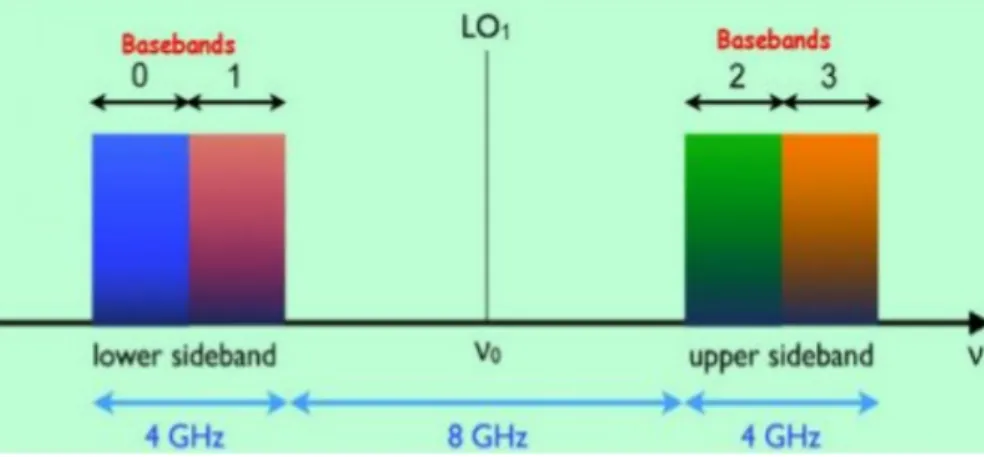
The IF and LO systems down-convert the sky frequencies to frequency bands of 0-2 GHz each. This work is realized in different stages. The first one splits the signal in the so-called upper sideband (USB) and lower sideband (LSB) in order to convert it to 4/8 GHz IF bands. The second down-conversion creates 2 GHz Basebands (BBs) that are allocated in USB and/or LSB. The spectral signal is divided into different spectral windows (SPWs), obtaining bandwidths up to 1.85 GHz. Then, the correlator operating mode will choose the number of channels in which the SPWs will be divided again, depending on the requested spectral resolution (Figure 2.5).
Figure 2.5: Schematic view of ALMA LO and IF system.
2.2.2
Back End and Correlators
The observed signals are down-converted, sampled, quantized in digitizers and then transferred to the correlator, which calculates cross-correlations and auto-correlations for each antenna pair and produces complex visibilities.
Correlators have two work modes: Time Division Mode (TDM) and Fre-quency Division Mode (FDM). The first one, TDM, provides wide bandwidth and low spectral resolution in continuum observations, while FDM allows a high spectral resolution. For this reason, for spectral-line observations the FDM is preferred .
2.2.3
Water Vapour Radiometer
The water vapour radiometer (WVR) observes the variations in the water vapour distribution in the troposphere that affect the observations. Phase
fluctuations (phase noise), which degrade the measurements at millimetric and submillimetric wavebands, are the effect of this variations. The WVR measures and estimates the amount of precipitable water vapour (PWV) along a given LoS to give the right phase corrections for each baseline. WVR measurements are taken on 1-second timescale to carefully sample the actual variations in the atmosphere. WVR is implemented on each 12-m antenna, but not on 7-m antennas (the compactness of the ACA baselines makes phase noise negligible).
2.2.4
Antennas and performance in Band 6
The observations analyzed this thesis were taken in Band 6. In the following we give an overview of the system and instrumentation in this Band.
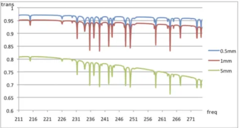
Band 6 covers the frequency range 211-275 GHz. It possesses dual side-band receivers, with the two sideside-bands available simultaneously, an IF fre-quency range of 5-10 GHz and a bandwidth of 7.5 GHz. This Band is affected by several narrow atmospheric absorption lines, most of which are from O3 (Figure 2.6).
Figure 2.6: Band 6 zenith transmission for PWV=0.5, 1 and 5 mm. Frequency is in GHz.
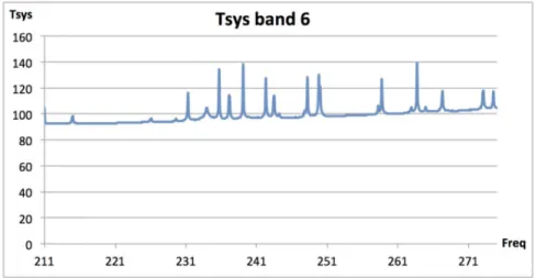
Figure 2.7: Typical Tsys at zenith for Band 6 with 1.262 mm PWV, based on
measured values of the receiver temperatures.
The system temperature Tsys is defined as (e.g. Jewell et al. 1997, ALMA memo series):
Tsys =
(1 + g)[Trx+ TA(sky)] ηeτ0sec z
where g represent the ratio of the gain response between the image and the signal, Trx is the receiver noise temperature (of the order of 50 K over most of Band 6), TA(sky) is the antenna-based temperature of the sky, η is the antenna efficiency, related to the maximum antenna gain and to the antenna power pattern, τ0 is the zenith optical depth of the atmosphere, sec z is the zenith secant which gives an estimate of the airmass at the observing elevation. The Tsys at Band 6 for PWV of 1.262 mm is shown in Figure 2.7.
Chapter 3
NGC 3100: ALMA
Observations and Data
reduction
This Chapter describes the ALMA observations obtained for NGC 3100 dur-ing Cycle 3 and the various step of the data reduction. The software used for data reduction and following analysis is CASA (Common Astronomy Soft-ware Application), version 4.7.0.
3.1
Observations
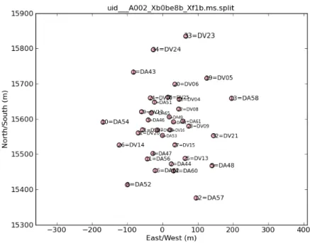
The observation of NGC 3100 was taken with the 12-m array in Band 6 (∼ 230 GHz) on March 22nd 2016 from 00:47:15.4 to 01:31:55.5 (UTC) with a total observing time of 44m 40s. 36 antennas were available and the array configuration had a maximum baseline of 460 m and a minimum baseline of 16 m. This corresponds to 0.65 arcsec of resolution and 10 arcsec of maximum recovered scale. Figure 3.1 shows the antenna configuration.
The used spectral configuration covered the frequency range 227 – 231 GHz and 240 – 244 GHz, divided in 4 SPWs:
• 3 SPWs of 128 channels with a total bandwidth of 2 GHz and a channel width of 15.6 MHz (∼ 20 km/s)
• 1 SPW of 1920 channels with a total bandwidth of 1.87 GHz and a channel width of 0.98 MHz (∼ 1.3 km/s)
Figure 3.1: Antennas configuration. Distance is in meter; dots represent an-tennas.
The radio quasar J1037-2934 was used as bandpass, phase and flux cali-brator. The amount of PWV range from 1.06 to 1.3 mm during the obser-vations and the Tsys is ∼ 80 K, on average.
3.2
Inspection and data calibration
3.2.1
CASA
Calibration, imaging and initial analysis of NGC3100 data were performed using CASA. This package has been developed to reduce interferometric data from modern radio telescopes such as ALMA and the upgraded VLA (or JVLA). It has a C++ core with an iPython interface. Its tasks and tools permit to deal with data from radio telescopes and to convert them in a so-called Meaurement Set (MS). The MS has a table-based structure with main and sub-tables, in which all the information is contained.
The principal MAIN table is divided in three columns. The raw visibilities are contained in the DATA column, the calibrated and model visibilities are stored in the CORRECTED and MODEL columns, respectly. At the end of the calibration, these three columns are completely filled.
3.2.2
Data import, inspection and flagging
Raw data from ALMA were transformed in MS through CASA task impor-tasdm. The so-called “a priori flagging” is applied on this MS. This editing removes data without specific inspection scan by scan. Data are identified and labelled based on the following reasons:
• Shadowing: depending on the elevation of the target, some antennas may obscure the ones behind them along the LoS, by reducing the effec-tive collecting area. This flagging recognizes and labels the visibilities affected by shadowing.
• Pointing: during the observation some scans are taken to verify the accurancy of pointing, which must be more accurate at high frequencies. These data are not used.
• Atmosphere: as for pointing, some scans are used to calibrate the at-mospheric effects during the observation.
• Autocorrelation: this is the result of the correlation of the signal of each antenna with itself. This flagging is necessary because noise due to systematic errors is amplified in autocorrelations and only cross-correlations between antennas are actually used.
3.2.3
A priori calibration
ALMA observations have to take into account two important factors related to the atmosphere and to the system noise: water vapour content and system temperature. In fact, the phase of visibilities are affected by the fluctuations in the troposphere, weather conditions and internal noise.
Fluctuations in the amount of PWV introduce a delay in baseline signals on short timescale (∼ 1 s, see Section 2.2.3) that needs to be removed. This can be done thanks to the WVR mounted on each antenna that measures the amount of PWV during all the observation. In Figure 3.2 the effect of the WVR corrections antenna by antenna is shown.
Figure 3.2: WVR corrections. The plots show the phase of the calibrator as function of time in SPW 3 in one polarization, for each antenna. Blue values are before WVR corrections, green values after them.
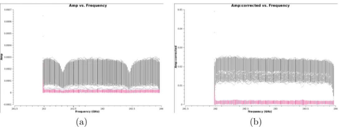
As seen in Section 2.2.4, the data are affected by the opacity of the atmosphere, by the antenna external temperature and by system noise. The corrections are taken into account through the Tsys calibration table. In Figure 3.3 it is possible to see how atmospheric effects on the visibilities were corrected by applying the Tsys table. In particular, it is possible to notice that the attenuation in correspondence of atmospheric lines disappear, and that the overall amplitude of the signal is rescaled.
(a) (b)
Figure 3.3: Tsys table corrections for SPW 2. (a) Visibilities amplitude vs
frequency without applying the Tsys correction table. (b) The same with Tsys
calibration table applied. Black lines are calibrator visibilities, while purple ones are NGC3100 visibilities.
After applying the WVR and Tsys tables, the MS was splitted in a new MS where only the target data are retained. Then, a new inspection of data allowed to identify possible corruptions in time and frequency. In particular, the edge channels of each SPW show high noise level during all observation. For this reason, the flagging of these channels was required.
3.2.4
Data calibration
The setjy task of CASA sets amplitude and phase for the flux calibrator, which is a source with known flux. This information is recorded in the MODEL column of the MS.
For the quasar calibrator J1037-2934, it was assumed a non-thermal model spectrum following
S = S0( ν νrest
)α
where S0 = 0.77J y is the specified flux density, α = −0.57 is the spectral index and νrest = 234GHz is the rest frequency.
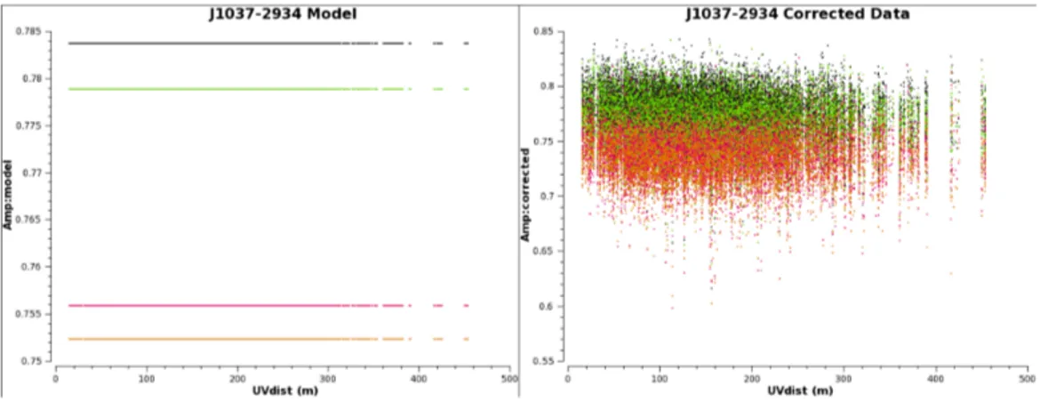
Figure 3.4 (left panel) shows the model (amplitude vs uvdist) for all SPWs. The model results flat, because the calibrator is a point-like source, and the amplitude changes for each SPW, because the model spectrum con-siders their different central frequencies.
Figure 3.4: Model (on the left) and corrected data (on the right) for J1037-2934. Amplitude vs. uv distance. Different colors correspond to different SPWs.
The Bandpass frequency-dependent gains B(ν) correct for amplitude and phase as a function of frequency, and are computed averaging in time. For this reason, the bandpass calibrator visibilities are firstly corrected by a time-dependent table to avoid phase corruptions on short timescales for each channel. Besides, this gives statistically significant solutions and it prevents from signal decorrelation. A gain factor table that contains short time-dependent solutions is found and it is applied “on the fly” to bandpass visibilities. The bandpass solutions, stable in time, are computed by an all-scan time integration to maximize the SNR. The bandpass calibrator is usually a quasar (QSO), where spectral lines are absent, and it is observed at the beginning of the run. In this case the same calibrator was used for flux and bandpass calibation (J1037-2934).
The gain factor table that contains long time-dependent solutions J (t) was found, using again J1037-2934 as calibrator. The source was regularly observed during the run, keeping it at the phase centre (so that it will have phase 0) in order to correct for atmosphere corruptions acting on phase and amplitude as a function of time.
These solutions are obtained using the CASA task gaingal.
Figure 3.5 shows two tables of gaincal solutions for amplitude and phase, respectively . The first one was obtained averaging the two polarizations, the second one was obtained for each polarization.
(a) (b)
Figure 3.5: Solutions for (a) amplitude and (b) phase as a function of time. Each plot corresponds to a different antenna.
3.2.5
Data examination
The final result of data calibration can be seen in Figure 3.6, where the calibrator and the source are plotted in black and purple, respectively. As explained, the radio quasar J1037-2934 has been observed in different scans. The first scan of the calibrator is the longest because it was used for bandpass calibration. The others are intended for phase calibration.
(a) (b)
Figure 3.6: Corrected visibilities of J1037-2934 and NGC3100. (a) The phase of visibilities as function of time, averaged for all channels. (b) The amplitude of visibilities as function of time, averaged for all channels. The calibrator is in black, NGC3100 is in purple.
Figure 3.7 shows the calibrator amplitude and phase as a function of frequency. It can be noticed that the spread of the 1290-channels SPW is wider, both in amplitude and phase.
(a) (b)
Figure 3.7: Corrected visibilities of J1037-2934. (a) Phase of visibilities as function of frequency, time-averaged. (b) Amplitude of visibilities as function of frequency, time-averaged. Plots are colourized by baselines.
Figure 3.8 shows the target NGC 3100 in the 1920-channel SPW. A double-horned line at the centre of the SPW is detected . The line is ob-served at ∼ 228.5 GHz, corresponding to the CO(2-1) emission line (νrest = 230.5 GHz) at redshift z=0.0088. The shape of the line suggests gas rotation.
Figure 3.8: Corrected amplitude visibilities of NGC 3100 in SPW 3 as a func-tion of frequency, time averaged. A double-horned line is detected in the centre.
3.3
Imaging
After the calibration, the data reduction continued through the imaging process.
3.3.1
Continuum image
A continuum image was obtained setting the clean mode to msf (Multi Frequency Synthesis) averaging all line-free channels. The central channels of SPW 3, from 228 to 229 GHz (where CO line is detected), and some channels of SPW 2 (high noise) were not considered for continuum imaging. The obtained image has a beam of 0.9800×0.7100, a RM S ∼ 0.1 mJ y beam−1 and a flux peak of 0.025 J y beam−1.
The continuum image shows a jet starting from the centre of NGC 3100 and extending towards the South direction (Figure 3.9). The northern jet seen with the VLA (See Figure 1.5) is not detected.
Figure 3.9: NGC 3100 continuum image. Resolution is 0.2 arcsec, noise level on the images is 0.1 mJ y beam−1. Contours from 4σ to 20σ with 10 levels.
Since this thesis is mainly focussed on the analysis of the CO line data cube, no efforts were attempted to obtain a better continuum image. Never-theless, a more accurate continuum image of NGC 3100 was obtained through self-calibration by Ruffa et al. (in prep.). Self-calibration is a technique to refine the target source calibration. Instead of an external calibrator, a model of the target is used to calibrate itself.
Figure 3.10 shows the new continuum image where both jets are now detected.
The previous continuum image in Figure 3.9 was able to show only the southern jet, because of its high level noise (∼ 0.1 mJ y beam−1). The self-calibration improves the RMS to 0.025 mJ y beam−1 and it makes both jets well visible.
Figure 3.10: NGC3100 continuum image self-calibrated. Both jets are detected. Resolution is 0.14 arcsec, noise level on the images is 0.025 mJ y beam−1. Contours from 4σ to 20σ with 5 levels.
3.3.2
CO line Image
A line image can be obtained using the task clean in channel/velocity mode in order to get an image cube (data cube), containing a defined number of 2-D images along the frequency/channel axis.
After having applied the CASA task uvcontsub to subtract the contin-uum flux from data, a channel image was obtained using natural weighting and setting the spectral resolution to ∆ν ∼ 10 M Hz (∼ 13 km/s). The re-sulting beam is 1.0100×0.7300; the noise level measured on an empty channel is ∼ 0.5 mJy beam−1. Figure 3.11 shows that the double-horned line spectrum turns into a ring in the channel map. In particular, the ring has blueshifted emission in the north region and redshifted emission in the south region with respect to the system velocity of 2592 km/s.
Figure 3.11: NGC3100 CO(2-1) line channel map. Spectral resolution is ∆ν ∼ 10 M Hz (∼ 13 km/s), noise level is ∼ 0.5 mJ y beam−1. Contours from 4σ to 20σ with 5 levels.
The integrated intensity map of the line (moment 0) and the integrated velocity map (moment 1) were extracted from this map (See Chapter 4). Moreover, this is the map used as input for the modelling of the velocity field of the molecular gas discussed in Chapter 5.
Chapter 4
NGC 3100: Data Analysis
This thesis is focussed on the analysis of the CO properties of NGC 3100, but important information on the interpretation of the results may come also from comparisons with radio continuum and dust emission.
4.1
CO line Moment Maps
A data cube can be most easily thought of as a series of image planes stacked along the spectral dimension (See Section 3.3.2). It is possible to collapse the cube into a moment image by taking a linear combination of the individual planes I(xi, yi, νk): Mm(xi, yi) = N X k νkm(xi, yi)I(xi, yi, νk)
where xi, yiindicate the i−th pixel of the plane of frequency νk. The moments are computed using a threshold which defines the range of pixel values of the data cube to include in the resulting map.
The integrated intensity map (moment 0) M0 can be written as:
M0 = N
X
k
I(xi, yi, νk)
and roughly represents the amount of gas present in each pixel as derived by summing the contributions from all spectral planes (column density).
The map was produced with a threshold of 4σ, and a noise level of ∼ 0.3 J y beam−1km s−1 is measured (Figure 4.1).
Figure 4.1: Integrated intensity map (moment 0). The RMS noise level is ∼ 0.3 J y beam−1km s−1. The wedge at the bottom shows the scale of the
map in J y beam−1km s−1. Contours from 4σ to 20σ with 5 levels.
The moment 0 map clearly shows the ring-like structure, already noticed in the channel maps. The major and minor axes of the ring are ∼ 8×4 arcsec2 or 1.5×0.75 kpc2. The ring appears inhomogeneous and even disrupted along the minor axis. Some additional emission is present outside the ring. This emission appears significant (> 4σ) and shows some correspondence with dust structures (See Section 4.3).
The integrated velocity map (moment 1) M1 is defined as:
M1 =
PN
k νkI(xi, yi, νk) M0
and represents the velocity field of the gas. It gives important information about the velocity range spanned by the gas and on the presence of velocity structures (i.e. the presence of preferred velocities at given positions).
Figure 4.2: Integrated velocity map (moment 1). The range of velocity is ∼ ±200 km/s around the Vsys = 2592 km/s. The threshold is set at 4σ.
The moment 1 map was derived with a 4σ threshold and is presented in Figure 4.2. The gas is distributed in a rotating disk that can be roughly divided in two parts: an upper blueshifted part and a lower redshifted part (See Section 3.3.2). The velocity spans a range of ∼ ±200 km/s around the systemic velocity (2592 km/s). However, some velocity irregularities seem to be present, perhaps indicating non-circular motions (See Section 5.2.4).
4.2
The CO as molecular gas tracer
The molecular gas mass in galaxies is dominated by molecular hydrogen, H2, but its strongly forbidden rotational transitions make it very difficult to directly detect it, unless shocked or heated to very high temperatures. For this reason, the emission from other molecules is usually used to trace the H2 in galaxies (Carilli & Walter 2013). The carbon monoxide (CO) is
the most abundant molecule in the interstellar medium (ISM) after H2, and emits strong rotational transition lines (occurring primarily through collisions with H2). Then, it can be considered as a “good” tracer of the molecular hydrogen.
The CO luminosity, LCO, is usually used to compute the total molecular gas mass (dominated by H2). It can be calculated from the CO moment 0 map. For NGC 3100 the integrated CO(2-1) line flux density was measured by summing the contributions from the five regions shown in Fig 4.3. This results in SCO = 42.82 ± 9.04 J y km s−1.
Figure 4.3: The five regions considered the measurement of the line flux den-sity. a) in green, 11.48 arcsec2; b) in red, 6.12 arcsec2; c) in blue, 0.4 arcsec2; d) in magenta, 0.64 arcsec2; e) in yellow, 1.28 arcsec2
Then, the luminosity LCO can be derived as integrated source brightness temperature following Solomon & Vanden Bout (2005) equation:
LCO = 3.25 × 10⁷( SCO J y km s1)( νobs GHz) −2( DL M pc) 2(1 + z)−3 [K km s−1pc2]
where νobs = 228.77 GHz is the observing frequency, z = 0.0088 is the red-shift and DL= 40.9 M pc is the luminosity distance. The resulting CO lumi-nosity is
The CO luminosity-H2 mass conversion equation is taken from Bolatto et al (2013):
M (H2) = αLCO M
where α is the so-called H2 mass-to-CO luminosity conversion factor, defined as the ratio of the total molecular gas mass in M to the total CO line luminosity. Different source populations have different values of α, because α is strictly dependent on the molecular gas conditions, such as its density, temperature and kinetic state.
For NGC 3100 we used α = 4.3 M [(K km s−1pc2)−1]. The resulting mass is M = 1.85 ± 0.4 × 10⁸M
, that is consistent with the mass computed from APEX observations (M = 1.5 ± 1.1 × 10⁸M
, Laing et al. in prep), re-ferring to a central 5 kpc region. This means that CO is mostly concentrated in the detected 1.5 × 0.75 kpc2 ring.
We notice that the conversion factor userd by Laing et al. was XCO = 2.3 × 1020cm−2(K km s−1)−1, where XCO is the conversion factor used to derive the molecular mass directly from the integrated fluxes. This value is very close to XCO = 2 × 1020cm−2(K km s−1)−1 , the value corresponding to α = 4.3 M [(K km s−1pc2)−1] (Bolatto et al. 2013).
4.3
Comparison with dust and radio
contin-uum
Figure 4.4 shows the dust absorption B-I image overlapped with the CO moment 0 map (red contours).
The CO ring-like structure nicely overlaps the inner semi-circular dust feature, suggesting the latter traces the same rotating structure. The other small detected CO regions do also tend to overlap with dust structures, sug-gesting the CO would trace the dust on much larger scales, but is not detected due to the fact that the present ALMA observations are not sensitive to scales larger than 10 arcsec (See Section 3.1).
Figure 4.4: Moment 0 map over the B-I dust image. Contours from 4σ to 20σ with 5 levels.
The radio jets from the central AGN can affect the CO line emission. They could be responsible for the partial disruption that affects the CO ring. This is supported by Figure 4.5, which shows that the radio jet axis approximately coincides with the minor axis of the CO ring.
Indeed the jets seem to fill the areas of the CO ring from which flux is lacking. If interaction is present between the jets and the CO gas, it follows that the jet axis is not perpendicular to the CO disk.
Figure 4.5: ALMA moment 0 map and continuum. Moment 0 in red, ALMA continuum in blue. Both contours start from 4σ to 20σ with 5 levels.
The ALMA radio continuum (230 GHz) is compared to three lower fre-quency observations from the VLA (5 and 8.5 GHz) in Figure 4.6.
Figure 4.6: Continuum image of ALMA and VLA. Contours for ALMA (black) observations start from 4σ to 20σ with 5 levels. Contours for VLA observations start from 5σ to 25σ with 5 levels at 5 GHz (red and green) and from 4σ to 20σ with 5 levels at 8.5 GHz (blue).
The emission at each frequency shows a very good matching. By com-paring the flux densities at the various frequencies, the spectral index of the various components can be inferred. As expected the core is flat, while the jets are steep (α = −0.7).
Chapter 5
Kinematics modelling of the
CO disk
To understand the kinematics and the morphology of the CO(2-1) rotating disk detected in NGC 3100, 3D models were built. The method chosen is the so-called tilted-ring model. Two softwares were used, TiRiFiC (Tilted Ring Fitting Code) and 3D-Barolo (3D-Based Analysis of Rotating Object via Line Observations) working with different algorithms. The modelling strategy of the two programs will be briefly described and the final results will be shown.
5.1
Tilted-ring model
The so-called tilted-ring model was developed for the first time for observa-tions of the neutral hydrogen (HI) emission-line (e.g. Rogstad & Shostak 1971) in the galaxy M83, to analyze the 2D velocity field in terms of a model consisting of hydrogen located in concentric rings rotating around the centre of the galaxy. The 2D tilted-ring model, also called bending model, is based on the assumption that the emitting material is confined to a disk and that the kinematics is dominated by the rotational motion (Rogstad et al. 1974). Each ring has a constant circular velocity Vrot(R), depending only on the distance R from the centre. The disk is therefore broken down into a number of concentric rings with different radii, that can have different inclinations, position angles and rotation velocities (Figure 5.1).
TiRiFiC and 3D-Barolo developed a more complex 3D tilted-ring model. In the 3D approach the full data cube is used to constrain the modeling (not only the 2D moment 1 maps). In addition instrumental effects are taken into account in the model through a convolution step. This has several
advantages; for instance it allows to remove artificial degeneracy between rotation velocity and velocity dispersion (e.g. line broadening). Unlike the 2D tilted-ring model, an analytic form for the fitting function in 3D does not exist and the model is instead constructed through Monte-Carlo extractions. Such techniques are known to be computationally expensive and they may converge to a local minimum of the function. In addition, a larger number of parameters is needed to describe the model with respect to the 2D case.
Figure 5.2: Geometrical parameters of the 3D disk model. The disk in the x0y0z0 space is projected into an ellipse in the xy plane of the sky. The inclination angle i is taken with respect to the plane of the sky, the position angle φ identifies the position of the major axis on the receding half of the disk and it is taken counterclockwise from the North direction
The 3D disk model is described by the following parameters (for each ring of radius R and width W , see Figure 5.2):
• spatial coordinates of the centre (x0, y0); • systemic velocity Vsys;