Application of multivariate statistical methods to the modelling of a flue gas treatment stage in a waste-to-energy plant

(1)

SCUOLA DI INGEGNERIA E ARCHITETTURA

Dipartimento di Ingegneria Civile, Chimica, Ambientale e dei Materiali

CORSO DI LAUREA MAGISTRALE IN INGEGNERIA CHIMICA E DI PROCESSO

TESI DI LAUREA in

Process Analysis for Energy and Environment

Application of multivariate statistical methods

to the modelling of a flue gas treatment stage

in a waste-to-energy plant

CANDIDATO Muratori Giacomo

RELATORE Ing. Antonioni Giacomo

CORRELATORE Ing. Dal Pozzo Alessandro

Anno 2017/2018 II sessione

(2)

(3)

Among all the flue gas components produced in Waste-to-Energy plants, acid air-borne pollutants such as sulfur dioxide, hydrochloric acid and other halogens hydrides (HF, HBr) have, depending on their toxicity and amount produced, the most rigorous emission standards provided by the European Parliament. Their removal is thus a key step of the flue gas treatment which is mainly achieved with the Dry Treatment Systems (DTS), technologies based on the direct injection of dry solid sorbents which is capable to subtract the acid from the gas stream with several important advantages and high re-moval efficiencies. However, the substantial lack of a deeper industrial knowledge makes difficult to determine accurately an optimal operating zone which should be required for the design and operation of these systems. The aim of this study has been there-fore the exploration, while basing on an essential engineering expertise, of some of the possible solutions which the application of multivariate statistical methods on process data obtained from real plants can give in order to identify all those phenomena which rule dry treatment systems. In particular, a key task of this work has been the seeking for a general procedure which can be possibly applied for the characterization of any type of DTS system, regardless of the specific duty range or design configuration. This required to overcome the simple mechanical application of the available techniques and made necessary to tailor and even redefine some of the available standard procedures in order to guarantee specific and objective results for the studied case. Specifically, in this so called chemometric analysis, after a pre-treatment and quality assessment, the process data obtained from a real working plant (Silea S.p.A., Valmadrera, Como, Italy) was analyzed with basic and advanced techniques in order to characterize the relations among all the available variables. Then, starting from the results of the data analysis, a linear model has been produced in order to be employed to predict with a certain grade of accuracy the operating conditions of the system.

(4)

(5)

Tra gli svariati composti volatili prodotti dai termovalorizzatori, gli inquinanti acidi come SO2, HCl e altri acidi alogenidrici(HF, HBr) hanno, data la loro tossicità e grandi quantità prodotte, i limiti di emissione più stringenti tra quelli previsti dal parlamento Europeo. La loro rimozione è quindi un passaggio chiave del trattamento dei fumi che si basa in gran parte sull’utilizzo di sistemi di trattamento a secco (DTS), cioè tecnologie basate sull’iniezione diretta di sorbente solido capace di sottrarre l’acido dalla corrente di gas con diversi vantaggi. Tuttavia, considerato anche il gran numero di possibili configu-razioni, sui DTS non è ancora stata raggiunta quella precisa ed approfondita conoscenza industriale che sarebbe necessaria per un’ottimale progettazione e funzionamento degli stessi. Lo scopo di questo studio è stato quindi, partendo da una fondamentale base ingegneristica, l’esplorazione delle possibilità che l’applicazione di metodi statistici mul-tivariati a dati ottenuti da processi reali possono dare per l’identificazione dei fenomeni che controllano il funzionamento di questi impianti. In particolar modo il lavoro si è concentrato sulla definizione di una procedura generale che possa essere applicata a pre-scindere dalla configurazione o dalla potenzialità dell’impianto e questo ha richiesto il superamento della semplice applicazione meccanica delle tecniche disponibili, rendendo anche necessario l’adattamento o la ridefinizione delle procedure in modo tale da garantire risultati specifici e oggettivi per il caso studio. Nello specifico, in questa cosidetta analisi chemometrica, dopo alcune valutazioni di tipo qualitativo, i dati di processo ottenuti da un impianto funzionante (Silea S.p.A., Valmadrera, Como, Italy) sono stati analizzati per mezzo di svariate tecniche in modo da poter caratterizzare le relazioni tra le singole variabili. Successivamente, partendo dai dati di questa analisi, un modello lineare è stato creato affinché possa essere impiegato per predire le condizioni operative del sistema.

(6)

1 Introduction 1

1.1 Waste to energy plants . . . 1

1.1.1 Acid gases . . . 2

1.2 Acid gas removal: Dry treatment systems . . . 3

1.2.1 The chemical process . . . 4

1.2.2 DTS configurations . . . 6

1.3 Aim of the study . . . 6

2 Material and method 7 2.1 Data pretreatment . . . 7

2.1.1 Data cleaning . . . 8

2.1.2 Data filtering . . . 8

2.2 Data analysis . . . 9

2.2.1 Quality of the data . . . 9

2.2.2 Preliminary evaluations . . . 11

2.2.3 Latent variable techniques: Principal Component Analysis . . . 13

2.3 Modeling . . . 16

2.3.1 Design of the model . . . 17

2.3.2 Empirical model from the literature . . . 19

2.3.3 Multiple linear regression . . . 19

3 Case study 21 3.1 Acid gas removal . . . 21

3.2 Process data . . . 22

3.2.1 Data pre-treatment . . . 23

3.2.2 Dataset subdivision . . . 25

4 Data analysis 27 4.1 Distribution and preliminary correlation analysis . . . 27

4.1.1 Discussion . . . 30

4.1.2 The inlet stream . . . 31

4.2 The reactor . . . 33

4.2.1 Applicability of the available conversion model . . . 33 vi

(7)

4.2.2 Filter reactivity potential . . . 34

4.2.3 Principal component analysis . . . 39

4.3 Discussion . . . 42

5 Modeling 43 5.0.1 The dependent variables . . . 43

5.0.2 The independent variables set . . . 43

5.0.3 Tuning and Validation . . . 44

5.1 HCL model . . . 45

5.1.1 Features tuning . . . 45

5.1.2 Results and discussion . . . 48

5.2 SO2 model . . . 50

6 Conclusions 53 A Supporting material 55 A.1 Case study . . . 55

A.2 Data analysis . . . 57

A.3 Modeling . . . 67

B Algorithms 71 B.1 Data cleaning and filtering . . . 71

B.1.1 Outlier detection . . . 71

B.1.2 Nan removal . . . 72

B.2 Empirical model fitting . . . 72

B.2.1 Empirical model . . . 72

B.2.2 Cost function . . . 72

B.2.3 Statistical fitting . . . 73

(8)

1.1 Scheme of a conventional waste incineration plant [1] . . . 2

1.2 Gas-solid shrinking core mechanism [2] . . . 4

1.3 Conversion model validation vs. literature bench scale data [5, Antonioni, 2011] . . . 5

2.1 Error examples: Outliers (red) and missing measure (yellow) . . . 8

2.2 Final process data after cleaning (red) and filtering (blue) . . . 9

2.3 Kurtosis comparison . . . 10

2.4 Time-series of two correlated variables . . . 12

2.5 Correlation scatterplot matrix . . . 12

2.6 Principal components in a two variables data set . . . 13

2.7 Loading plots: (a) Single PC (b) Bivariate . . . 16

2.8 Real trend of the data (black) and overfitting model (blue) . . . 18

2.9 PLS matrix representation . . . 20

3.1 DTS section of the Valmadrera plant . . . 22

3.2 Rayleigh probability distribution function . . . 24

3.3 Probability distributions: (a) rs (b) χ . . . 26

4.1 Total retained variance . . . 31

4.2 PC1 and PC2 bivariate loading contribution plot . . . 32

4.3 Inlet stream: PC3 loading contribution plot . . . 32

4.4 Model calibration vs. case study process data (1 day average) . . . 33

4.5 Case study instantaneous measures: (a) χHClvs. rs chart and (b) Process data vs. model prediction . . . 34

4.6 The bicarbonate accumulation at time t . . . 35

4.7 PCs absolute gain vs k . . . 36

4.8 Loading comparison for PC2 at k = 0 and k = 18 . . . 37

4.9 Loading comparison for PC1 at k = {0, 9, 18, 69} . . . 37

4.10 R2 of the monovariate regression of HClout on BICin . . . 38

4.11 Result of the varimax rotation . . . 40

4.12 PC2 mono variate contribution plots . . . 41 viii

(9)

5.1 Fitting performance vs N◦of features: (a) No range correction, (b) With

range correction . . . 45

5.2 Variables weights for the five features - eight variables PLS model . . . 47

5.3 Variables weights comparison . . . 48

5.4 Model prediction vs process data: (a) Outlet HCl flow [kmol/h], (b) HCl conversion . . . 49

5.5 Fitting performance vs N◦of features: (a) No range correction, (b) With range correction . . . 50

5.6 Variables weights for the five features PLS model . . . 51

A.1 Reconstruction of a 2 minutes and a 10 minutes windows . . . 55

A.2 Probability distributions: (a) rs and (b) conversions χ. Time series, rs (blue) and conversion χ (orange) : (c) second set and (d) zoom . . . 56

A.3 Probability distributions: (a) rs (b) χ . . . 57

A.4 First scatterplot matrix, 13 variables . . . 58

A.5 Inlet stream: PC1 loading contribution plot . . . 59

A.6 Inlet stream: PC2 loading contribution plot . . . 59

A.7 PC1 time series representation, moving average at 180 minutes . . . 60

A.10 Overall retained information at PC4, Total variation . . . 61

A.11 Model calibration vs. process data (1 day average)[6, Antonioni, 2014] . . . . 61

A.12 Total retained variance . . . 61

A.13 Loading contribution plots for the first four PCs . . . 62

A.14 Total retained variance . . . 62

A.15 PC1 mono variate contribution plots . . . 63

A.18 First trajectory mono variate loading contribution plot . . . 64

A.19 Second trajectory mono variate loading contribution plot . . . 65

A.20 T1 time series representation, moving average at 180 minutes . . . 65

A.21 T3 time series representation, moving average at 180 minutes . . . 66

A.24 T1 T3 and PC4 probability distributions . . . 67

A.25 PC2 probability distributions . . . 67

A.26 Fitting performance comparison on the CV set: three features vs five features 68 A.27 Features tuning: Fitting performance comparison on the V set . . . 68

A.28 Fitting performance of the final model on the T set: sample from Jul 27 to Jul 30 . . . 69

(10)

1.1 Daily average emissions concentration ranges (mg/Nm3). . . 1

1.2 Daily and half-hourly average emission limit (STP, standardized at 11 % oxygen in waste gas) . . . 2

1.3 Typical operational ranges for Temperature, stoichiometric ratios SR and reagent mass flow M [1]. . . 3

2.1 Eigenvalues and retained variance (example) . . . 14

2.2 Linear regression model . . . 19

3.1 Process variables and units . . . 22

4.1 Variables and their statistics parameters . . . 28

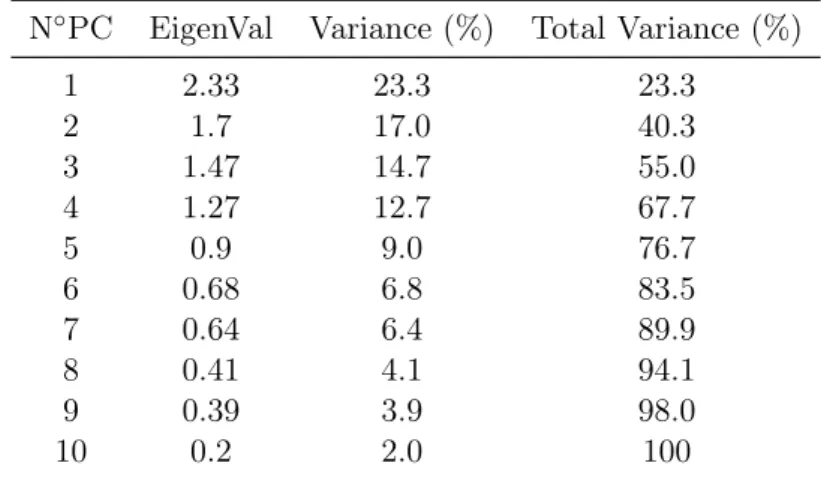
4.2 PCA results . . . 31

4.3 PCA results . . . 39

5.1 PC2 subset statistics . . . 44

5.2 R2 vs N◦of features . . . 46

A.1 Quality of the data and cleaning operation recap . . . 56

A.2 PCA results . . . 57

(11)

Introduction

1.1 Waste to energy plants

Volume and hazard reduction of the waste produced by human activities is funda-mental to lower the environfunda-mental, social and economic impact that an untreated waste could induce. Concerning this, incineration is part of a wide range of complex treatment processes that allow the overall management of the of wastes that arise in society. Incineration is a Waste to Energy (WtE) process that burn and decompose substances in waste in presence of oxygen while recovering energy and reducing thus the use of fossil fuels and the CO2 production. This allows to pursue the volume reduction of

waste together with the capture (and concentration) or destroying of potentially harm-ful substances such as the ones already present in the waste or the ones derived by the combustion process. Indeed, the waste incineration process transfers about the 80% of the burnt matter into the flue gas that is mainly composed of CO2 and water, together

with a mix of many other components, showed in the next table (Tab.1.1) as typical concentration ranges in waste flue gas.

CO TOC Dust HCl HF SO2 NOx Hg Cd PCDD/F

<10-30 1-10 1000-5000 500-2000 1-10 150-400 200-500 0.1-0.5 0.1-0.5 1-10

Table 1.1: Daily average emissions concentration ranges (mg/Nm3).

The atmospheric emission of these components is harmful for human health and ecosystem integrity and thus emission limits are provided from the qualified authorities. Each single pollutants in the flue gas have then to be reduced from the concentration of the combustion chamber to the required emission standards. This is done through a series of abatement stages that are called air pollution control (APC) systems and come right after the combustion chamber and before the emission in atmosphere. Commonly an APC train (Fig.1.1) starts with the removal of the fly ashes directly downstream the boiler, then the next steps are the neutralization of acid gases, the NO_x removal and a final polishing step aimed to remove all the left pollutants like mercury and low volatile organic compounds such as dioxins.

(12)

The European emission standards are given by the Industrial Emissions Directive (IED) of the European parliament[4, 2010/75/EU] together with the criteria for the de-termination of the best available technologies (BAT) which must be used for the APC systems to reach these standards.

Figure 1.1: Scheme of a conventional waste incineration plant [1]

1.1.1 Acid gases

Among all the flue gas components, depending on their toxicity and amount produced, acid airborne pollutants such as sulfur dioxide, hydrochloric acid and other halogens hydrides (HF, HBr) are the ones listed in the IED which have the most rigorous emission standards. HCl especially, is obtained from the decomposition of inorganic chlorides

and organic chlorine compounds (PVC etc.) that are highly present in wastes and,

without a correct abatement strategy, incineration would be its major emission source to the atmosphere. Air emission limit values concerning waste incineration plants are reported from the IED in table 1.2 as daily average emission limit and half-hourly average emission limit for the 97% of the overall operation time (B) and with a possible exceeding in emission in the 3% of the measures given in (A).

Emission limit (mg/Nm3) Daily A (100%) B (97%)

Hydrogen chloride (HCl) 10 60 10

Hydrogen fluoride (HF) 1 4 2

Sulphur dioxide (SO2) 50 200 50

Table 1.2: Daily and half-hourly average emission limit (STP, standardized at 11 % oxygen in waste gas)

(13)

1.2 Acid gas removal: Dry treatment systems

Acid gas removal can be pursued by several processes which are classified as wet, if the acid react with a neutralizing agent in liquid phase, or dry/semi-dry, if the neutralizing agent is a solid or a wet solid. Until 2000s the process standard for this type of application was the wet scrubbing but, since mid-1990s, dry treatments have been demonstrated to be cost-effective, easy to operate and to be maintained[1] and then have gradually substituted the more obsolete technologies.

In DTSs acid pollutants are subtracted from the gas stream through the reaction with some alkaline powders which can be divided in two main categories, the calcium based and the bicarbonate based system, which have different costs, reactivity and working conditions.

Slaked lime (Ca(OH₂)) is obtained through the calcination and hydration of the limestone (CaCO3) and due to its high availability and low cost it is the most used reagent in these

type of applications. Lime has lower reactivities than other types of reagents but some high porosity refined types are produced at higher costs through specific processes which guarantee higher reactivities. For Ca based systems the optimal working temperature window is between 120◦C and 160◦C, with a performance increase proportional to the decreasing of temperature, due to the effect that the higher relative humidity induces on the particle core, enhancing the reactivity.

Bicarbonate based alternatives are largely widespread and rely on the Solvay registered NEUTRECTM process, which employ Solvay synthesized sodium bicarbonate (NaHCO₃) as reagent. The latter, despite its higher reactivity, is more costly than the Ca based reagents but its final process residues can be regenerated and re-used. These systems, differently from the Ca alternatives, follow a classical kinetic increase from 140◦C to 300◦C, due to classical kinetic factors. Find in table 1.3 a comparison recap of different technologies.

T [◦C] SR (HCl) SR (SO2) M [kg/waste ton]

Wet systems

60-65 1.02-1.15 12-18

Dry systems

Ca based 120-160 1.1-1.5 1.3-3.5 20-30

NaHCO₃ 140-300 1.04-1.2 15-18

Table 1.3: Typical operational ranges for Temperature, stoichiometric ratios SR and reagent mass flow M [1].

(14)

1.2.1 The chemical process

Slaked lime is capable to neutralize acid gases with a single step reaction: Ca(OH)2(s) + 2 HCl(g) → CaCl2(s) + 2H2O(g)

Ca(OH)_2(s) + 2 HF_(g) → CaF_2(s) + 2H2O(g)

Ca(OH)2(s) + SO2(g) + 1₂O2(g) → CaSO4(s) + H2O(g)

Ca(OH)_2(s) + CO_2(g) → CaCO_3(s) + H2O(g)

The NEUTRECTM process follows instead two steps where firstly, at temperatures above 140◦C, NaHCO₃ releases CO₂ and water in a so called "pop corn effect" decom-position that gives a sodium carbonate (Na2CO3) powder which, given its high specific

surface, is much more reactive than the starting bicarbonate and can then neutralize the acid gas.

NaHCO_3(s) → Na₂CO_3(s) + CO_2(g) + 2H2O(g)

Na2CO3(s) + 2 HCl(g) → 2NaCl(s) + H2O(g)

Na2CO3(s) + 2 HF(g) → 2NaF(s) + H2O(g)

Na2CO3(s) + SO2(g) + 12O2(g) → NaSO4(s) + CO2(g)

Solid-gas reaction model

For all types of reagents the heterogeneous gas-solid reaction can be easily carried-on in one single step with fast operations but, differently by wet scrubbing, kinetics are much more un-promoted. The process follows in fact a so called "shrinking core mechanism" (Fig.1.2) where the acid gradually consume the sorbent particle and creates a product layer on it.

Figure 1.2: Gas-solid shrinking core mechanism [2]

The thickening of the gathering product layer slows down the fresh core reaction and does not allow the full depletion of the sorbent, making thus essential to account for a quantity of reagent which is bigger than the stoichiometric need, leading then to a larger reagent consumption and a higher production of final residues.

(15)

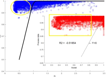
These complex phenomena have been studied[5, Antonioni, 2011] for the reactions of hy-drogen chloride and sulfur dioxide with sodium bicarbonate, leading to the production of a conversion model that is capable to predict the removal efficiency of acid gases as a function of the rate of solid reactant:

χ = rs

n_{− rs}

rsn_{− 1} (1.1)

As can be seen from the equation, the acid pollutant conversion χ is expressed as a function of two parameters:

• rs: is a dimensionless parameter correspondent to the ratio between the effectively dosed reagent and the one which is stoichiometrically needed. Starting from the reactions reported in the previous section it is possible to write it as:

rs = N aHCO3in

N aHCO3st

= N aHCO3in

HClin+ 2SO2in+ HFin

(1.2)

• n: is an adjustable parameter which is proportional to the removal efficiency of the system. This is a lumped parameter which gathers all the chemical phenomena occurring in the system and the operating conditions affecting the reaction (e.g. temperature, contact time, particle size etc.).

Figure 1.3: Conversion model validation vs. literature bench scale data [5, Antonioni, 2011]

The previous figure (Fig.1.3) refers to a model validation carried out on bench scale

data[7, Brivio, 2007] and it shows a very good agreement of the model equation with

exper-imental data, confirmed by a coefficient of determination R2 > 99% for both the HCl and SO2 predictions.

(16)

1.2.2 DTS configurations

Possible DTS configurations are several and highly customized depending on the amount and types of waste burnt. Acid gas removal is usually the first pollution control step after the furnace and for this reason the injection of the powders occurs right after the air pre-heating system and, in some cases, after a humidification pre-conditioning. Then, once the stream has been sprayed, it is sent to the de-dusting step, commonly performed through a cyclone or a fabric filter, which can work also for the removal of the particulate and flying ashes coming from the furnace. In case that fabric filters are used alkaline reagents settle on the membrane while creating a fixed bed where the gas pass through and the reactions keep going on, leading thus to an overall increasing of the abatement performance. Starting from this basic configuration it is possible to customize the system for example by changing the injection point or with the use of a humidification pre-conditioning system. Actual design trends push then toward the use of multiple stages systems that use both bicarbonate and slaked lime and which, if properly operated, have been demonstrated to require a lower amount of solid reactants than a single-stage process[5].

1.3 Aim of the study

Generally speaking DTSs can be considered simple and versatile plants which are cost-effective, easy to operate and to be mantained. This, together with the easiness of solid residues disposal and the absence of operating issues (such as the "rain-out" at the chimney), make DTSs the preferable solutions in most of the cases.

However, particularly in case of multiple stages solutions, these systems suffer of a sub-stantial lack of a deeper industrial knowledge[5] which makes difficult to determine ac-curately safe operating zones, leading then to the necessity to operate with high excess of reactants that leads naturally to a surplus production of residues and consecutive dis-posal costs. Actually, the reported model (eq.1.1) demonstrates its applicability for the prediction of the DTS conversion on large time averaged windows[5], but its single lumped parameter makes it not very flexible to briefly changing operating conditions and thus not capable to produce reliably instantaneous predictions. For this reason, even in light of the increasingly lower emission standards, the aim of this study is the exploration of some of the possible solutions which a chemometric analysis on real process data can give. Like all the chemical treatment processes in fact, air pollution control systems in WtE plants are equipped with process control instrumentation where data are measured at high frequencies in order to be employed in monitoring and control. These data however represent a great deal of information that by means of multivariate statistical methods can be extracted and employed to identify all the DTS ruling phenomena and try to produce a model which is capable to produce reliable instantaneous predictions.

(17)

Material and method

Chemometrics is the application of mathematical and statistical tools on a chemical system in order to characterize the mutual relations among the available measures and study the state of the system. Usually this approach is applied to on-purpose designed experiments that are performed on controlled conditions and where high precision data are collected with high reliability. In this specific case however, process data are not produced primarily for the chemometric analysis, so they must be checked and cleaned since they must follow specific requirements of type, ordering and quality. After this, the big quantity of correlated and redundant informations characteristic of the process derived measures makes necessary, in addition to the classical visual and basic statistical analysis, the use of advanced statistical techniques that allow a deeper elaboration and are capable to extract the essential informations from the dataset, allowing then to proceed with a final regression analysis aimed to the estimation of a model for the process. This model can then be employed to predict with a certain grade of accuracy the system state allowing then to optimize the operating conditions. In this chapter, techniques which have been demonstrated to be useful in this work are introduced without any claim to be exhaustive in the presentation of the broad range of methods which are effectively available.

2.1 Data pretreatment

All the measurements from DCS are available in large quantities, are subjected to many types of error and, in case that these inconsistencies are not detected and correctly removed, this will end easily in a misunderstanding of the data trends which can even make impossible the analysis and modeling. In particular it is possible to spot four types of error which are characteristic of sensor measurements:

• Outliers: by definition these are the measures which fall out from the normal measures trend and for this reason they can be easily spotted and removed; They take part to this type of error any zeros and unjustified peaks measures.

(18)

• Missing measures: measures holes in the process data consist usually in 10÷20% of the overall availability.

• Gross errors: are commonly related to a wrong calibration of the sensor and they are easily spotted and conceptually avoidable (e.g. measured inlet and outlet flow rate in an equipment don’t close the mass balance).

• Random error: this is the so called noise, it is unavoidable and hopefully small so that a proper filter is capable to remove it without affecting the real measure.

2.1.1 Data cleaning

Before to start the analysis and modeling of the data, previous mentioned wrong data must be identified and corrected such that the final results are consistent and conciliated each other. Usually, wrong data can be manually spotted through a visual control on the data charts (Fig.2.1) but in case of large quantities of data or for on-line applications a computational approach is necessary. Hence, it is essential to create some algorithms that allow to detect, remove and substitute wrong measures with values that are much more likely to be consistent with the surrounding measures and process constraints and thus help the next analysis to be more correct. Big windows of missing measures cannot be reconstructed reliably and for this reason they force the subdivision of the dataset in more subsets which anyway could turn out to be useful in the regression analysis for the creation of training and validation sets.

Figure 2.1: Error examples: Outliers (red) and missing measure (yellow)

2.1.2 Data filtering

Once data have been re-constructed it is then necessary to smooth out short-term fluctuations and thus remove the noise of the sensor through a filter that can have a more or less sophisticated approach.

The most simple filtering method is the moving average, where each measure is substi-tuted by the average of the previous or next (or both) measured n-terms. The larger is the width of window average, the stronger is the filter and thus the higher is the capacity to remove random errors but with an higher loss in information. Filtering works also as a polishing step to assimilate better into the data trend those measures that have been added during the cleaning phase to substitute some wrong measures.

(19)

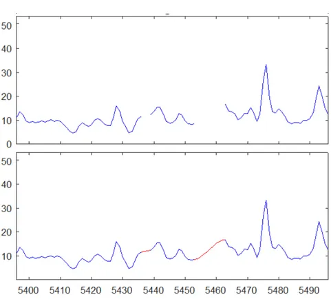
Find in the next figure (Fig.2.2) the effect of a moving average filter on the cleaned version of the previous example (Fig.2.1).

Figure 2.2: Final process data after cleaning (red) and filtering (blue)

2.2 Data analysis

High complexity of the process data can make very difficult to understand the back-ground of the observed phenomena. This, in addition to the availability of advanced modeling tools, could induce the analyst to pass directly to the modeling phase without trying to give a meaning to the starting observation, ending thus in models that, despite even outstanding results, cannot be explained. Data analysis includes all those tech-niques that, through a more or less deeper elaboration, allow to explore also the most complex systems so that it is possible to:

• Suggests hypotheses about variables correlations which, on an expertise base, can be demonstrated as causalities;

• Help to make assumptions;

• Support the selection of more advanced statistical techniques; • Provide a basis for further data collection;

In this specific case the main purpose of the analysis is to characterize the type and the influence of each variable on the system state and so can be considered successful if all the necessary statistical tools are correctly employed to characterize the system, understand what are the independent variables that truly affect its state and finally determine their type of influence on it.

2.2.1 Quality of the data

Chemometric analysis on real working systems finds an important advantage in the easy and the high availability of the data. The latter however are not produced intention-ally to be analyzed and, depending on their characteristics, it can be more or less easy to obtain meaningful results. Indeed, the most common techniques employed in the regres-sion analysis rely on the fact that each variable should vary enough so that it is possible

(20)

to study its variation related to the one of the other variables. This characteristic is not obvious for process variables which instead in some cases can assume almost constant values or are kept intentionally on specific set points by the control system. Moreover, it is common for many statistical methods to rely on the normal distribution of the ana-lyzed data and, in case this is not verified as it is common for process variables, the final result ends to be biased. Nevertheless, these are intrinsic and unavoidable circumstances and in these cases the only possible solution is the preliminary characterization of all the variables probability distribution so that, at the end of the analysis, it is possible at least to discern real poor result from the ones dependent on the bad conditioning of the dataset.

The probability distribution

The distribution of the variables measures can be evaluated either visually with his-tograms or through specific parameters called simple moments of the distribution. The first two moments, the mean µ and the standard deviation σ, are the basic parameters which define the Gaussian normal distribution that fits at the best way the variable set. While the first gives the absolute order of magnitude of the measure, the second quantify the dispersion of the variable set.

In case of a multi-variable dataset it is better to refer to the relative standard deviation σ∗ = σ_µ (called also coefficient of variation) which is a quantification of the scale of the variable and allows to compare different variables. Many mathematical and statistical tools are sensitive to the relative scaling of the variables and require to bring the whole dataset to a common scale by means of a so called normalization process. The most used normalization method is the standard scores evaluation where each variables sets is transformed through eq. 2.1 in order to have zero mean and standard deviation equal to one.

X∗ = X − µ

σ (2.1)

The skewness γ (3rd moment) and the kurtosis k (4rd moment) allow to characterize the deviation of the variable distribution from the normality.

(21)

The kurtosis k in particular is an important parameter which allows to estimate, for a given variability expressed by σ∗, if the probability distribution is more or less squeezed toward the mean. If a distribution is characterized by an high kurtosis it means that, related to a normal distribution which have the same σ, a bigger part of the measures are concentrated nearer to the center and a small part of those are, as a counterbalance, as much far from the mean as low it is their number. In process derived variables, assuming that true outliers have been fully removed, high kurtosis are usually characteristic of measures which are mostly constant but experience few justified measure peaks. This makes the measure disadvantaged in a correlation analysis on the base of its intrinsic lack of variability and even more depending on the next normalization. Indeed, the fact that the normalization procedure relies only on the first two moments neglecting the possible absence of normality, makes high kurtosis a detrimental factor in the analysis and, being formally equal in σ∗, the variables which are characterized by an higher kurtosis, and are thus more squeezed toward the center of the distribution, are subjected to a variance reduction which is higher than the one which should be really needed due to their true distribution.

2.2.2 Preliminary evaluations

The regression analysis starts with the application of basic techniques aimed to the preliminary evaluation of the possible correlations/causalities and to start making hy-pothesis and assumptions. This, in case of complex systems, is not intended to fully determine the system but is essential so that, once the data are analyzed with advanced techniques, it is possible to understand better the results. In particular, this phase is necessary to identify those correlations that, although they lies naturally in the dataset, are supposed to be irrelevant for the study and need to be clearly recognized in the next steps of the analysis in order to avoid misunderstandings.

Data visualization

The first preliminary step for the analysis of a complex system is the representation of the data. Effective visualization in fact makes complex data more accessible, yet understandable and usable. A human can distinguish differences in size, shape, position, orientation and color readily without significant processing effort and thus a correct visualization set up allow to perform particular analytical tasks. It is easy, once data are represented through an effective way, to make comparisons, spot correlations, support the selection of more advanced statistical tools and confirm or refute any other results.

In this perspective, process data time-series (Fig.2.4), captured over a period of time, are the first step to understand how operations affect that measure, vice-versa and also to spot possible correlations in case that two or more variables are superposed in the same chart.

(22)

Figure 2.4: Time-series of two correlated variables

Then, if some correlations are spotted, they can be further studied with correlation plots, that are bivariate representations which, in case of multivariate evaluations, are called scatterplot matrices (Fig.2.5). Many other representations are possible through histograms, bar charts and other advanced representation tools in order to rank and cat-egorize the effect of any real or on-purpose created variables or to quantify the frequency distribution of the latter.

Figure 2.5: Correlation scatterplot matrix

Correlation indexes

Despite the proved effectiveness, plot shapes are not always fully understandable and, as it is common for bivariate representation of process data, can appear messy and confused. For this reason in order to better detect possible correlations it could result necessary to associate visual representation to an absolute correlation index. The correlation between two measures is a statistics which express how much, if the first variable varies, the second is likely to vary itself. The most used parameters capable to quantify the grade of correlation among two variables (x, y) is the Pearson’s correlation coefficient, that represent how much the relation between x and y can be described by a linear function:

rx,y =

cov(x, y) σxσy

(23)

This statistics is parametric, meaning that it is preliminary assumed that the analyzed variables are normally distributed. Of course this is not generally the case for process variables and for this reason it is worth to use the Spearman correlation coefficient, which is non-parametric and assesses how well the relationship between the two variables can be described using a monotonic function:

ρx,y =

cov(rgy, rgy)

σrgxσrgy

Pearson and Spearman results ranges from -1 to 1 which implies respectively full direct or indirect monotonicity. In case that the value is zero it means there is no correlation.

2.2.3 Latent variable techniques: Principal Component Analysis

Chemical processes plant are heavily instrumented by sensors that measure variables at high frequencies. This makes available a large amount of data that, even though they can be considered a great resource, are characterized by a big quantity of correlated and redundant informations that even if relevant for some control systems may not affect significantly the whole process. For this reason a preliminary elaboration aimed to remove unnecessary informations and extract the essential ones is fundamental. A common approach to this so called "data mining" is to think the whole variables dataset as a n multi-dimensional space where each measure is represented on a different space dimension. In case that some correlation or redundancy exists, it is possible to state that the effective dimension of the space on which the process data vary can be reduced. Latent variables techniques (LVs) are some algebraic methods that allow to rearrange the multidimensional space to find, in order of importance, those new dimensions called latent variables, on which the information is maximized (Fig.2.6).

(24)

Different LVs approaches differ in the way the LVs are selected. After the determina-tion of a proper LVs set it is possible to operate a compression while choosing only the first (n − l) LVs that retain the largest amount of information. By this way problems of process analysis, monitoring, and optimization are greatly simplified and also multi-variate systems, that differently are difficult to be represented, can be visually explored. Moreover, a deeper analysis on the LVs and on the transformation matrices allows to perform a correlation analysis on the raw variables.

Principal Component Analysis (PCA) is a popular multivariate latent variable tech-nique that can be successfully applied to analyze and monitor continuous processes. Mathematically speaking, PCA relies on the eigenvector decomposition of the covariance matrix of the X dataset consisting of m measures of the n variables:

cov(X) = X

T_X

m − 1

The eigenvectors of cov(X), the so called principal components (PCs) and are usually

determined through a singular value decomposition. PCs are ordered depending on

the magnitude of the correspondent eigenvalue so that the first accounts for the space trajectory with the largest possible variance, and each succeeding component in turn, orthogonal to the previous, has the highest variance possible.

This basic approach is called covariance PCA but, in case that the X matrix is pre-liminary column-wise normalized to the standard scores, which is the most common case in process data which do not have a common scale, then all the raw variables are by def-inition characterized by unit variance. Then equation 2.2.3 coincides with 2.2.2, cov(X) is called correlation matrix and the technique becomes the so called correlation PCA. In this case algebraic and geometrical interpretation are the same but the normalization allows to focus the analysis on the correlations without any bias given by the dataset scale.

Choice of the number of PCs

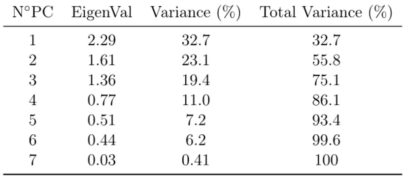
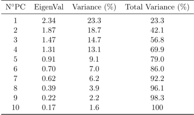
The size of each eigenvalue can be associated to the number of variables which have been lumped in that specific component. By following this definition it is possible then to calculate a PC percent retained variance as the ratio among the size of its eigenvalue and the overall sum of the eigenvalues. Then, if the singles retained variances (%RV) of each PCs are summed up in order, it is then possible to evaluate the cumulative retained variance (%CRV) (see the next example Tab.2.1).

PC Eigenvalue %RV %CRV 1 2.3 46.03 46.03 2 1.61 32.11 78.14 3 0.58 11.68 89.82 4 0.42 8.44 98.27 5 0.09 1.73 100

(25)

Once the retained variances have been calculated it is then possible to exploit the results to, firstly have an overall evaluation of the amount of the system redundancy and subsequently to select a suitable number of components that is capable to reproduce cor-rectly the system without loosing essential information. Most common selection methods are:

• The first method relies on the CRV chart where, as can be seen from the next figure, in case that the raw system was highly correlated and redundant, it is possible to spot a "knee" in the curve. This knee correspond to a serious drop in retained variance, as can be confirmed in the table (Tab.2.1), and thus the number of PCs correspondent to it is conventionally chosen as a reasonable number of dimensions capable to compress the system.

• The choice of the minimum number of the PCs can be done also through a cross validation. Here the principal components are firstly determined on a training set and then the Root Mean Square Error is calculated between the real variables of a validation set and their reconstruction (Eq.2.2) through a k specific number of PCs. The k number of PCs that gives the minimum error on the cross validation is then taken as reference.

• Two other possible "fast" methods define the last good component either as the last that have a retained variance bigger than 5% or the last which have the corre-spondent eigenvalue bigger than one.

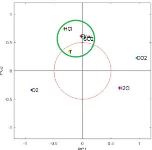
The loading analysis

The PCA procedure allows to represent the X dataset through the new space basis as follows:

X = t1pT1 + t2pT2 + ... + tkpTk + E (2.2)

Here p are the eigenvectors which correspond to the direction cosines of the orthogonal rotation associated to the PCA transformation and for this reason they have unity norm. If the eigenvectors are multiplied by the square root of their corresponding eigenvalue then they are called loadings and they are proportional to the standard deviation expressed by that trajectory. The coordinates t represent the projections of the X raw components in the new reference system and are called scores while E, the residual matrix, contains all the information rejected while compressing the dataset to a lower dimensionality.

(26)

The loadings and the scores are fundamental parameters that allow to analyze the system and characterize correlations among the starting raw variables. Indeed, each element of the loading vector represents the effective contribution of that raw variable on that principal component and this allows first to label that PC as dependent from a single phenomenon (e.g. a PC which is highly contributed by all the temperatures of the process can be labeled as the "process temperature" PC) and then allows to spot correlations among the raw variables depending on the fact that variables which contributes strongly to the same PC (see stars in Fig.2.7) are for sure correlated (or anticorrelated).

Figure 2.7: Loading plots: (a) Single PC (b) Bivariate

These evaluations can be facilitated with bivariate or 3D loading representation but, in case of high number of variables, it can still be difficult to interpret the contribution plot. In these cases, if two or more PCs appear to be strictly related depending on the mu-tual presence of important contributions of the same variables, it can be worth to perform a further rotation of that analyzed subspace in order to ease the final interpretation[18]. Among several types of rotations the most common is the orthogonal varimax one which works simply by maximizing the variance on the orthogonal axes of the analyzed sub-space.

2.3 Modeling

The last step of the chemometric analysis is the production of a mathematical model for the analyzed chemical system. Modelling procedures are divided in white or black box approaches depending on the amount of a priori information which is available. White-box models are created only on the base of predetermined information while black-White-box models returns a results but their functional form is neither known nor predetermined. Chemometric modeling is an hybrid approach between the two where, once a plausible structure for the model has been designed starting from the preliminary assumptions, the available data are used to train the model and fit its parameters.

(27)

2.3.1 Design of the model

The design of the model usually starts once the variables which affect most the state of the system and their specific influence on the latter are determined. Nevertheless, it can happen that the data analysis is not capable to clarify completely the roles of some variables and in this case the modeling phase need to assume also a validating purpose. Variables which have a specific role in the prediction of the system state are called predictors and, once they are arranged inside the model, they build, together with the constant parameters, its structure. A part from these, the model is defined also by its hyperparameters, constant values that define its structure and, whereas they are external to the model, cannot be estimated directly from the data. This is the case for example of the number of features in a linear regression or the exponents grade in a polynomial regression.

Modeling procedure

Once all the internal and external parameters have been individuated they need to be estimated so that the model is capable to reproduce reliably future data.

This is done through three steps:

1. Training: the parameters of the all the possible models solutions are statistically fitted by minimization of the prediction error on a so called a training data set. 2. Tuning: the performances of the different solutions are then compared by

evalu-ating their error on a new independent set called cross-validation set.

3. Validation: the solution that ensure the best performance on the cross-validation set needs finally to be tested on a third independent set called validation set in order to be sure that any over-fitting is avoided. The crucial point of this set is that it should never be used to choose among two or more solutions, so that the error on this set provides an unbiased estimate of the generalization error.

Modeling subsets

The previous listed process makes necessary the subdivision of the available dataset in order to check and counter-check all the assumptions on different and independent data series. A common rule for the dataset subdivision is that the training set is made up of the 60-80% of the available measures while the left part is divided among tun-ing and validations. This subdivision must be done consciously so that all the three independent sets are equally representative of the same dataset probability distribution because, differently, the performances on the singles dataset would not be comparable but dependent on the specific represented population.

(28)

Estimation of the model performance

During the training in order to minimize the prediction error or during the tuning and validations procedures, if two or more solutions are available and need to be compared or in case that some hypothesis need to be tested a tool for the estimation of the goodness of the model is necessary. This can be done with some indicators that have different characteristics:

• Coefficient of determination R2

This coefficient is largely used in the context of statistical models and accounts for the proportion of the variance of the real variable, taken from the dataset, which is predicted from the modeled variable:

R2 = 1 −SSres SStot = 1 − P i(yi− fi)2 P i(yi− ¯y)2

Where SS_res and SS_tot, defined as above, are respectively the residual sum of squares, which accounts for the model missed variance, and total sum of quares which accounts for the overall variance of the real predicted variable.

R2 gives an absolute estimation of the goodness of the model with a maximum of 1, which correspond to full prediction, decreasing values from 1 to 0 which stand for a decreasing capacities of prediction and values below 0 whcih mean that the model is not working.

• Errors

Mean Square Error (MSE), Root MSE (RMSE) and Mean Absolut Error (MAE) are all possible estimation of the mean distance among the real measures and the ones predicted from the model. Errors are sensible to the scale of the measure and allow only to compare different solutions.

(29)

Over-fitting is a common misfitting phenomenon (See Fig.2.8) which is spotted if the model is wrongly designed so that it produces optimal predictions on the training set but it predicts poorly new additional independent datasets such as future observations. This is common in those models where the number of features is over sized related to the effective variability of the modelled system.

2.3.2 Empirical model from the literature

Empirical models for the studied chemical system can be already available from the literature. In that case, if the features of the model can be estimated directly from the available dataset it is possible, through a statistical fitting procedure, to estimate its parameters. Then its performance can be evaluated through the mentioned methods and, in case of bad or misleading results, the model can be uploaded and further validated depending on available informations.

2.3.3 Multiple linear regression

If an empirical model is not available, among the broad range of multivariate mod-eling techniques, Multiple linear regression (MLR) is one of the most simple and easy interpretable models. It is a hybrid model where the structure is assumed to be linear a priori but the constant parameters are estimated from the process data:

Y = Θ0+ Θ1F1+ Θ2F2+ ... + ΘnFn

Table 2.2: Linear regression model

In the previous equation Θi are the model parameters while Fi are the so called

features of the model. Notice that Θ0 is a constant parameter called ’bias term’ which

does not refer to any feature. Partial least squares regression

Linear regression models that works with large numbers of variables are often sub-jected to over-fitting phenomena which, given that the model features should be the on-purpose selected predictors, cannot be solved with the discard of any of those, mak-ing then impossible to prevent this misfittmak-ing phenomenon.

This problem can be solved while taking advantage of the possible rotation of the dataset space in order to concentrate as much information as possible in the first k principal components which guarantee the model to not overfit the predicted variable. The key point of this linear modeling procedure, called Partial Least Square regression (PLS), is that the rotation is performed on the predictors variables space not only while pursuing the maximization of the variability on this space but also while maximizing the correlation of the the found PCs with the matrix of the dependent variables, which in case they are more than one are decomposed on their principal trajectories too.

(30)

Figure 2.9: PLS matrix representation

Formally, if X and Y are the independent and dependent variables sets represented on the raw reference system, then they can be re-written generically as X = T PT + E and Y = U QT + F . In case of PLS, T and U are the variables sets represented in the new compressed reference system which is chosen so that:

max[corr2(U, T ), var(U ) ∗ var(T )] (2.3)

Once this new "modeling conscious" reference system has been determined, the number of features of the model is chosen as an hyperparameter and all the discarded information is condensed inside the residual matrices E and F .

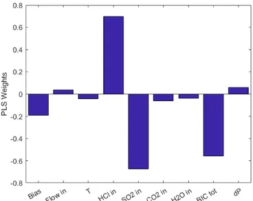
PLS produces very simple models that, if correctly validated, can give good results with a very low computational expense. Moreover, in addition to the system state predic-tion, the model features and parameters can be exploited for an integrative investigation of the dataset through the analysis of the loadings and of the θ weights referred to the starting raw variables, which quantify the grade of proportionality among that predictor and the system state.

The θ weights are obtained while considering that the PLS model written as Y = HQT (with Q the set of chosen PCs and H their respective weights) can be written equiva-lently as Y = XθT. From this equivalence θ is seen as the projection of Q on the raw system and can be written as θT = P QT, where P is the loading matrix compressed to the maximum k PCs spotted with the tuning of the model.

(31)

Case study

This work is based on the process data obtained from the Silea S.p.A. waste to energy plant located in Valmadrera, Como, Italy. All the reported plant specifications are obtained from [10]. The plant works on two lines (line 1 and line 3) which can treat respectively 6 waste ton per hour and 9.5 waste ton per hour, mainly divided in municipal waste and treated biomedical waste. Both lines are based on the same layout: furnaces with heating recovery systems and APC systems which are composed by a DTS, a NO_x removal section and then a final wet scrubbing section.

3.1 Acid gas removal

Acid pollutants are removed in both lines with a double reagent injection (Fig.3.2) but only one de-dusting stage. The first injection consists of a solid alkaline powder named DepurcalTM MG, a dolomitic sorbent where Ca(OH)₂, thanks to the properties of magnesium oxide (MgO), which actually does not take part to the neutralization reaction, can be sprayed directly inside the furnace at high temperatures (800-1400◦) without the relative drawbacks. The pre-treated flue gas with exhausted lime is then sent, after heat recovery, to the reaction tower of the DTS where activated carbon and bicarbonate powders are sprayed with a pneumatic transport. Here after a mean residence time of 2 seconds, treated stream is then sent to a fabric filter for de-dusting. Fabric filter in this case is constituted by several internal cells which works independently, allowing then to exclude one of them for maintenance without stopping the equipment. Singles cells cleaning is done instead during the operations with compressed air through pulse jet technique that uses full immersion valves. The reaction continues on the solid which accumulates on the membrane until the residues are removed, gathered in a heated hopper and carried to a storage silo. This work is aimed to the analysis of the bicarbonate DTS stage comprehending the plant section which starts after the pre-heating system and ends after the fabric filter.

(32)

Figure 3.1: DTS section of the Valmadrera plant

3.2 Process data

The chemometric analysis performed in this work is based on the availability of pro-cess data from line three. Here, in addition to many propro-cess variables measurement systems, three FTIR sampling points are positioned after the furnace (before the DTS reaction tower), after the fabric filter and before the chimney. The first (FTIR1) and second (FTIR2) in particular, which are reported in figure (Fig.3.2), are exploited in this work for the analysis of the inlet and the outlet composition to the bicarbonate DTS stage. FTIR instrumentation is capable to detect several different compounds composi-tions which are used by the Distributed Control System (DCS) to control the dosage of the reagents and then sent to the Emission Monitoring System (EMS). Other essential process data for this work are stored in the DCS and include the flue gas flow rate, its temperature, the bicarbonate feed flow rate and the pressure differential at the fabric filter, actually a measure of solid residues accumulation on the membranes, see the recap in the next table (Tab.3.1). All the available data have been sampled from 27/07/2015 h1.01 to 12/08/2015 h23.38, with a frequency of one minute, for an overall amount of sampling for each variable of 24419 measures.

T Gas NaHCO3 dP HCl SO2 HF CO NO2 CO2 O2 H2O ◦_C _Nm3/h _kg/h _kPa _mg/Nm3 _mg/Nm3 _mg/Nm3 _mg/Nm3 _mg/Nm3 _{% vol} _{% vol} _{% vol}

(33)

3.2.1 Data pre-treatment

This work has started with a preliminary analysis on the quality of available data. From a first evaluation it is clear that several measures are missing due to temporarily mis-functioning, voluntary stops or lack in the storage of the data. This is true espe-cially in case of FTIR measures which are characterized by several windows of missing numbers or zeros measures (spotted by the outlier seeking algorithm), which last from some minutes to even 6 hours. In particular in the analyzed period it is possible to spot: • A big series of very brief stops which are randomly encountered in both the FTIR

sensors.

• The periodical occurrence, each 646 minutes of windows of missing numbers of 9 minutes firstly in FTIR1 and then after 53 minutes of 10 minutes in FTIR2. Those are probably, due to the regular periods and windows length, an automatic reset or calibration.

• Starting from the 03/08/2015 h 09.30.00 to 06/08/2015 08.40.00 a series of long missing measures windows which occur alternatively or simultaneously in both the FTIR sensors. These are probably due to an unwanted stop and necessary fix or to a wanted maintenance on the instrumentation.

While the first two types of windows can be substituted with the reconstruction algo-rithm quite accurately, the long windows cannot obviously be reconstructed because of their width and for this reason the whole dataset between the 03/08/2015 h 09.30 to 06/08/2015 h 08.40 need to be discarded. This so created big hole in the data availabil-ity however may be exploited in a modeling perspective for the creation of the needed modeling subsets.

Outliers removal, reconstruction and filtering algorithms

After the selection of the dataset, its cleaning has been pursued through two main algorithms aimed to the detection and conversion of outliers in missing measures (NaN) and to the subsequently substitution of all the NaN values with a new value, consistent with the previous and the next terms. This procedure results to be necessary only on the

FTIR compositions measures since process data from the DCS (T, gas feed, NaHCO3

feed, dP) are highly accurate and do not seem to present anomalies.

The outlier removal is done in two main steps. Firstly, for each variable set, a statis-tical distribution of the measures is estimated and then, once the probability distribution function is available, it is possible to choose, either manually or through an algorithm, a tolerance factor which is the minimum probability for a measure to not be an out lier. In this case the tolerance factors has been chosen manually for each variable starting from a visual representation of the data. See the algorithm in appendix B.

(34)

Compositions measures, due to the high heterogeneity of the burned waste, are highly variable and usually present high and sharp peaks while, on the contrary, it is common for outliers to show up as zeros or very low unjustified measures. For this reason the probability distribution function is fitted as a Rayleygh function which, as can be seen from the next figure (Fig.3.2), is zero in zero and more tolerant on the high measures.

Figure 3.2: Rayleigh probability distribution function

The reconstruction of the data is then done through the scanning of the singles

variable sets. Every times the NaN removal algorithm found a an hole in the dataset it measure its width and it choose three variables before the starting and after the finish of the window. This data are then used to determine an interpolation curve (with interp1 Matlab function) that allows finally to calculate all the missing values as the ones which are more likely to joint the hole extremes. Nota bene that this algorithm is tailored on this specific dataset where it is known that data holes are rare and not nearer than three measures. This allows to estimate the interpolation curve without any check on the effective availability of three measures before and next the hole but, in a more general interpretation, the latter must be provided. See the algorithm in appendix B. Find in figure A.1 an example of data reconstruction.

Data filtering is finally applied on the data after the data reconstruction to remove

random errors. This is done through a moving average with a window width of 10

minutes, a good compromise between noise removal and the left true signal. Find in the table (Tab.A.1) a recap of the cleaning operations.

(35)

3.2.2 Dataset subdivision

Starting from what is stated in section 2.3 the dataset needs to be divided in three independent subsets that are equally explicative of all the possibles states of the systems. Nevertheless, this requirement follows a general modeling standard which, given that in this case the available data are time series not produced on purpose, cannot be precisely satisfied in terms of represented population if the three subsets are obtained by the simple splitting in consecutive time series.

In order to obtain the best possible subdivision a distribution analysis needs to be performed on such variables that are as most explicative of the process as possible. At this purpose the assembled variables defined in 1.2.1, the rs and the conversion, are supposed to be appropriate.

The dataset, as it is justified in 3.2.1, is already subdivided in two main subsets due to the missing of important informations from the 03/08/2015 h 09.30 to the 06/08/2015 h 08.40. Unfortunately, the distribution analysis on these two preliminarily subsets gives soon a first problem and, as can be seen from the figure (Fig.A.2) especially in the case of the conversion, the two subsets cannot be overlapped in terms of probability distribution. This misfitting, as it is clearer in the time series, is due to an anomaly in the second set, from the 10/08/2015 h22.36 to the 11/08/2015 h07.36, due to unusual low dosage of bicarbonate related to the amount which should be needed depending on the inlet amount of acid. Here in fact the rs persists stable under the unity for about nine hours and as a consequence the DTS experiences a substantial drop in conversion. After this phase a sharp peak in the rs is experienced, meaning that at that point the systems restart to work, it detects an anomalous amount of acid in the outlet and thus it feed an high amount of bicarbonate.

Concerning the modeling procedure this part of the dataset is not in compliance with the required standard and for this reason needs to be discarded. These so created subsets have the probability distributions represented in figure A.3. As it is clear subset 2 is still biased from some operations problems which do not allow to have a stable distribution of the rs and thus of the final conversion. After a detailed study these anomaly has been ascribed to a possible inconsistency among the measure of the fed bicarbonate, which is an input to the process, and the real dosed bicarbonate which, in case of malfunctioning of the dosing system can be different. Starting from this possible explanation subset 2 have been completely discarded with a final result which can be seen in figure 3.3 which represent three main subsets:

1. Training set: from 27/07/2015 h1.01 to 04/08/2015 h7.48 and from 06/08/2015 h 08.40 to 08/08/2015 h 11.29 correspondent to the 66.7% of the dataset.

2. Cross-validation set: from 08/08/2015 20.07 to 11/08/2015 h14.46 correspon-dent to the 22.3% of the dataset.

3. Validation set: from 11/08/2015 h14.47 to 12/08/2015 h 23.38 correspondent to the 11% of the dataset.

(36)

Figure 3.3: Probability distributions: (a) rs (b) χ

This so obtained distributions are, as expected, not perfectly comparable but this result is considered acceptable and the 66.7-22.3-11% dataset subdivision is perfectly within the standard ranges. However, further checks will be carried on once more ad-vanced results are available from the data analysis.

(37)

Data analysis

The data analysis starts after the assembling of the dataset based on some preliminary assumptions:

• All the non-acid outlet compounds (CO, NO₂, O₂, CO₂, H₂O) and the inlet CO and NO2 are irrelevant for the process and are then neglected.

• The oxygen, even if it takes part in the sulfur dioxide neutralization, it is usually neglected on the base of its high excess. In this case however it is maintained because it is an important estimator of some correlations trends hidden among the inlet variables which depends on the combustion process and need to be spotted and eventually ignored if irrelevant.

• The carbon dioxide is involved in the bicarbonate decomposition and it is then necessary to evaluate if its presence among the combustion products is relevant for the DTS performance.

• Water is involved in many of the process side reactions which, together with the moistening of the powder, could influence the DTS performance and need then to be analyzed.

• The temperature and the pressure differential have been selected from the available process database because they could represent a good information source to be exploited respectively in the reactor kinetic analysis and in the influence of the fabric filter on the whole abatement performance.

• All the left variables are supposed to be influential on the process.

4.1 Distribution and preliminary correlation analysis

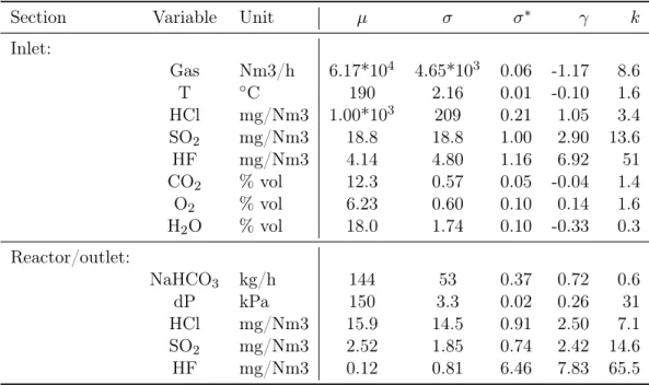
The left variables are supposed to be influent on the DTS system but needs to be analyzed through a distribution probability analysis in order to evaluate their measure quality, the amount of carried information and thus determine their capability to be correlated each other. In the next table (Tab.4.1) the mean (µ), absolute (σ) and relative standard deviation (σ∗) together with the kurtosis (k) are reported to assess the statistical distribution of each variable.

(38)

Section Variable Unit µ σ σ∗ γ k Inlet: Gas Nm3/h 6.17*104 4.65*103 0.06 -1.17 8.6 T ◦C 190 2.16 0.01 -0.10 1.6 HCl mg/Nm3 1.00*103 209 0.21 1.05 3.4 SO₂ mg/Nm3 18.8 18.8 1.00 2.90 13.6 HF mg/Nm3 4.14 4.80 1.16 6.92 51 CO2 % vol 12.3 0.57 0.05 -0.04 1.4 O₂ % vol 6.23 0.60 0.10 0.14 1.6 H₂O % vol 18.0 1.74 0.10 -0.33 0.3 Reactor/outlet: NaHCO₃ kg/h 144 53 0.37 0.72 0.6 dP kPa 150 3.3 0.02 0.26 31 HCl mg/Nm3 15.9 14.5 0.91 2.50 7.1 SO₂ mg/Nm3 2.52 1.85 0.74 2.42 14.6 HF mg/Nm3 0.12 0.81 6.46 7.83 65.5

Table 4.1: Variables and their statistics parameters

After a standard score normalization the mutual correlation can be visually analyzed through a scatter-plot matrix (Fig.A.4) and parametrically by means of bivariate corre-lation Spearman coefficients. Find in the next paragraphs the results and comments of these applied techniques.

Inlet gas flow

T HCl(in) SO2(in) HF(in) CO2(in) O2(in) H2O(in) NaHCO3(in) dP HCl(out) SO2(out) HF(out)

Gas(in) 0.32 0.21 -0.03 -0.06 0.01 -0.03 -0.04 0.17 0.28 0.07 0.07 -0.03

From a first visual inspection it is clear that the inlet gas flow measures lies generally on a squeezed band. The low variability, confirmed by the high kurtosis, is due to the process control operations and makes more difficult to spot correlations even with more advanced techniques.

From the correlations analysis it is possible to spot that the only clear but obvious effects are experienced on the pressure drop in the fabric filter and on the bicarbonate dosage in the reactor while all the left measures, in particular T and HCl_(in), are possibly related but need a further analysis.

(39)

Inlet acids

Gas(in) T HCl(in) SO2(in) HF(in) CO2(in) O2(in) H2O(in) NaHCO3(in) dP HCl(out) SO2(out) HF(out)

HCl(in) 0.17 0.06 1 0.20 0.23 -0.16 0.016 -0.22 0.45 0.11 0.18 0.13 0.13

SO2(in) 0 -0.16 0.20 1 0.49 0.18 -0.15 -0.08 0.30 -0.05 -0.48 0.13 0.01

HF(in) -0.06 -0.13 0.23 0.49 1 -0.07 0.09 0 0.14 -0.03 -0.23 0.06 -0.01

The three inlet acids compositions are analyzed together depending on their high mutual correlation, confirmed also by their obvious direct proportionality with the bi-carbonate dosage due to the control system based to one or all these three compositions. HCl, as it is confirmed from table 4.1, is present in larger quantities than the other two acids and its kurtosis confirm the visual impressions of a good variability.

On the contrary SO_2(in) and HF result from the distribution chart lower and squeezed, which is confirmed, especially in case of HF, by the very high kurtosis. This means that burnt waste is less rich in compounds which produce these kind of products but many peaks of concentration are experienced. As can be clearly spotted from the bivariate plots, while each single acid is obviously correlated with its outlet measure, HF_(in) and especially SO_2(in) demonstrate a strong anti-correlation with HCl_(out).

Other inlet variables

CO2(in) 0.05 0.13 -0.16 0.17 -0.07 1 -0.93 0.44 0 -0.09 -0.18 -0.13 0.21

O2(in) -0.07 0.16 0.02 -0.15 0.09 -0.93 1 -0.27 -0.07 0.07 0.14 0.14 -0.15

H2O(in) -0.04 -0.04 -0.22 -0.08 0 0.44 -0.27 1 -0.15 -0.14 -0.03 -0.08 0.23

Among these variables carbon dioxide and oxygen show the most eye-catching relation in the whole matrix plot and it is also clear that a linearity of these two takes place with the water inlet composition. All the three measures, accordingly to their distribution parameters and to the visual inspection, have a good variability. This results in many spotted possible relations that needs a further analysis.

Temperature and pressure differential in the fabric filter

T 0.31 1 0.06 -0.16 -0.13 -0.13 0.16 -0.04 0.03 0.15 0.16 0.07 -0.02 dP 0.28 0.15 0.11 -0.05 -0.03 -0.09 0.09 -0.14 0.04 1 0.09 0.02 0.12

The temperature, even though it is low variable, given its low k and γ can be con-sidered well conditioned. On the contrary, the pressure differential has a very high k and this can justify the poor results for correlation coefficients. In addition to the ones previous mentioned (dP vs Gas_(in) and T vs Gas_(in)) some other possible, but not clear, relations are experienced but not confirmed with many variables. The two variables do not demonstrate preliminarily an influence on the outlet acid but a further analysis is required.