An application of the extended Kalman filter to the attitude control of a quadrotor

(1)

POLITECNICO DI MILANO

Corso di Laurea Magistrale in Computer Engeneering Dipartimento di Elettronica, Informazione e Bioingegneria

AN APPLICATION OF THE EXTENDED

KALMAN FILTER TO THE ATTITUDE

CONTROL OF A QUADROTOR

Advisor: Prof. Matteo MATTEUCCI Co-Advisor: Dott. Andrea ROMANONI Co-Advisor: Prof. Marco LOVERA

Master thesis by: Leonardo ASCORTI, ID 745919

(2)

(3)

List of Figures

1 First prototypes of manned quadrotors. . . 19

2 The Parrot AR.Drone, a commercial smartphone-controlled quadrotor. 20 1.1 Model of the quadrotor with two Cartesian reference frames. . . 27

1.2 Visual representation of the Euler angles . . . 30

2.1 Pre-existing Simulink model. . . 46

2.2 Simulink model of the dynamics block.. . . 48

2.3 Simulink model of the control block. . . 48

2.4 Simulink model of the DC motors block. . . 49

2.5 Partial view of the updated Simulink model.. . . 51

2.6 Simulink model of a generic MEMS sensor. . . 52

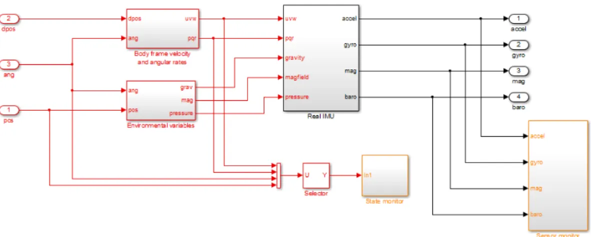
2.7 Simulink model of the IMU block. . . 53

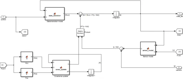
2.8 Simulink model of the continuous time EKF. . . 54

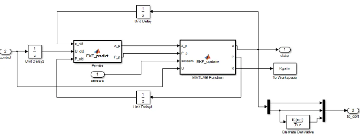
2.9 Simulink model of the discrete time EKF. . . 55

2.10 Simulink model of the discrete time EKF. . . 57

3.1 Hovering simulation . . . 62

3.2 Altitude variation: the desired trajectory (red) and the actual one (blue). . . 63

3.3 Altitude variation: state variables and estimates. . . 64

3.4 Linear movement: the desired trajectory (red) and the actual one (blue) of the pitch angle. . . 65

3.5 Linear movement: state variables and estimates. . . 65

3.6 Rotation around the Z axis: the desired trajectory (red) and the actual one (blue) of the yaw angle. . . 66

3.7 Yawing movement: state variables and estimates. . . 66

3.8 Complex trajectory: variables and estimates. . . 67

3.9 Continuous time ﬁlter performance with diﬀerent values of the mag-netic inclination. . . 69

3.10 Discrete time ﬁlter performance with diﬀerent values of the magnetic inclination. . . 70

3.11 Estimated linear velocity components with diﬀerent magnetic decli-nations. . . 71

(6)

3.12 Stability of the closed loop simulation using anti-aliasing ﬁlters of diﬀerent orders. . . 72 3.13 Trajectories of the state variables in closed loop: hovering. . . 74 3.14 Trajectories of the state variables in closed loop: linear movement

with altitude variation.. . . 76 3.15 Actual trajectory of the quadrotor in the case of two perpendicualr

segments. . . 77 3.16 Trajectories of the state variables in closed loop: two perpendicualr

segments. . . 78 3.17 Trajectories of the state variables in closed loop: diagonal movement

with altitude variations. . . 80 3.18 Hovering simulation with errors in the Kalman ﬁlter parameters:

con-tinuous time ﬁlter estimates. . . 82 3.19 Hovering simulation with errors in the Kalman ﬁlter parameters:

dis-crete time ﬁlter estimates. . . 83 3.20 Hovering simulation with errors in sensor axis misalignment

calibra-tion: continuous time ﬁlter estimates. . . 85 3.21 Hovering simulation with errors in sensor axis misalignment

calibra-tion: discrete time ﬁlter estimates. . . 86 3.22 Hovering simulation with errors in sensor biases calibration:

contin-uous time ﬁlter estimates. . . 87 3.23 Hovering simulation with errors in sensor biases calibration: discrete

time ﬁlter estimates. . . 88 3.24 Closed loop simulation of a complex trajectory with sensor calibration

(7)

List of Tables

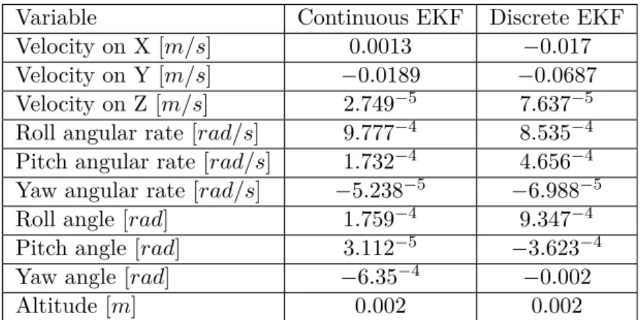
3.1 Default parameters used in the simulations. . . 60 3.2 Mean values of the estimated variables (hovering). . . 61 3.3 Mean value of the extimated roll angles with diﬀerent magnetic

incli-nations (discrete time EKF). . . 68 3.4 Drift values in hovering condition of the closed loop system after 10

seconds. . . 73 3.5 Coordinates of the end points of the diagonal trajectory. . . 79

(8)

(9)

Acknowledgements

I am very grateful to my advisor, prof. Matteo Matteucci, who supported me through all the stages of the development of my work, not only with great competence, but also with remarkable courtesy and patience. I would also like to acknowledge my two co-advisors, dott. Andrea Romanoni and expecially prof. Marco Lovera, his knowledge and experience in aerospace engeneering was fundamental for this thesis. A special thank goes to dott. Marco Bergamasco, who built the quadrotor that inspired this research during his PhD course.

(10)

(11)

Abstract

The focus of this thesis is the application of the extended Kalman ﬁlter to the attitude control system of a four-propellers unmanned aerial vehicle usually known as quadrotor.

The Kalman filter is a mathematical tool well suited for an algorithmic imple-mentation that estimates the state of a dynamic system influenced by random noise given a set of measurements which are also corrupted by random noise. If the system and measurement eqautions are linear functions of the state variables and the noises are both normally distributed, the filter can be proven to be an optimal estimator. In practice, the linearity conditions are often not satisfyed, but some rielaborations of the filter algorithm have been used for more than fourty years in many nonlinear applications with good results. The extended Kalman filter (EKF), used in this thesis, is one of the first and best known nonlinear filter versions.

A quadrotor is a helicopter lifted and propelled by four rotors. Small sized quadrotors are often used as UAVs (unamanned aerial vehicles) in research and am-ateur projects, because of the simple symmetric structure and relatively easy control law with respect to traditional helicopters. In this thesis, the extended Kalman ﬁlter is applied to estimate the state of the quadrotor from the noisy measurements of on board low-cost MEMS sensors. The estimated state is intended to be used by a control algorithm (not discussed in this work) to maintain the desired attitude during various maneouvers.

The EKF is implemented in Simulink in both continuous and discrete time, as an extension of a pre-existing model, which simulates the dynamics and control of a quadrotor. The performance and stability of the system is then analyzed with many test cases, from simple hovering to complex trajectories, both with open and closed loop control. The model is also tested for robustness in case of errors in the measurements of physical parameters and incorrect sensor calibration.

(12)

(13)

Estratto in lingua italiana

Lo scopo di questa tesi è l’applicazione del ﬁltro esteso di Kalman (abbreviato EKF) al sistema di controllo dell’assetto di un elicottero quadrirotore.

Il filtro di Kalman è uno strumento matematico, facilmente applicabile in forma di algoritmo, per stimare lo stato di un sistema dinamico perturbato da rumore sulla base di un insieme di misure anch’esse corrotte da rumore. Il filtro in pratica è in grado di compensare i due tipi di errore per ottenere una stima migliore di quella che potrebbe essere ottenuta conoscendo solo il valore delle misure o il modello del sistema dinamico. Nel caso in cui sia il sistema dinamico sia le equazioni che descrivono le misure sono funzioni lineari delle variabili di stato ed entrambi i rumori sono generati secondo distribuzioni gaussiane, è possibile dimostrare che il filtro di Kalman è uno stimatore ottimo. I sistemi reali difficilmente soddisfano queste condizioni, in particolare per quanto riguarda la linearità delle equazioni, tuttavia la ricerca in questo campo ha sviluppato varianti del filtro originale che forniscono risultati soddisfacenti (sebbene non ottimi in senso stretto) anche quando applicati a sistemi non lineari. In particolare, in questa tesi è utilizzato il filtro di Kalman esteso, uno dei primi algoritmi non lineari che negli anni è stato applicato a con successo in diversi scenari, tra cui la guida automatica di veicoli ha una particolare rilevanza.

I quadrirotori sono un tipo di velivolo senza pilota (UAV) a decollo e atterraggio verticale (VTOL) che ha suscitato notevole interesse tra i ricercatori negli ultimi anni, perché le leggi che ne governano il volo sono relativamente semplici rispetto a quelle degli elicotteri propriamente detti e anche la loro realizzazione ﬁsica è consi-derevolmente meno complessa, dato che essi non hanno parti meccaniche come pale inclinabili o ﬂap, ma si manovrano esclusivamente variando la velocitá dei quattro rotori e presentano comunque una buona agilitá di movimento. Tra le varie aree di ricerca che coninvolgono questi velivoli, ha particolare importanza lo sviluppo di algoritmi e leggi di controllo, sia per l’assetto sia per la navigazione.

In questa tesi, il filtro esteso di Kalman è impiegato per stimare lo stato del velivolo in base alle misure fornite dai sensori di tipo MEMS a basso costo presenti a bordo. Lo stato cos� stimato è poi utilizzato dal sistema di controllo (il cui funzio-namento non è discusso in questa sede) per mantenere l’assetto richiesto nel corso delle manovre di volo. Il modello completo del quadrirotore, dei sensori e del filtro di Kalman è implementato in Simulink e i risultati di diverse simulazioni con differenti

(14)

condizioni sono analizzati per studiarne le prestazioni, la stabilità e la robustezza agli errori.

Nel Capitolo 1 si ricava il modello matematico del sistema dinamico, sulla base di leggi ﬁsiche e aerodinamiche. Il modello prevede uno stato del sistema composto da dieci variabili:

• le velocità lineari lungo i tre assi cartesiani nel sistema di riferimento del velivolo;

• le velocità angolari attorno ai tre assi cartesiani nel sistema di riferimento del velivolo;

• l’orientamento del velivolo rispetto ad un sistema di riferimento esterno, espres-so in angoli di Eulero (rollio, beccheggio e imbardata);

• la quota rispetto al terreno.

Nello stesso capitolo si ricava anche il modello dei sensori, sulla base delle loro caratteristiche generiche. Questo modello comprende delle costanti che devono essere deﬁnite in sede di calibrazione. Da ultimo, i modelli del sistema e dei sensori sono linarizzati (calcolandone la matrice jacobiana), come richiesto dall’algoritmo EKF.

Il Capitolo 2 è dedicato alla descrizione del modello Simulink utilizzato per le simulazioni. Il modello è composto da una parte preesistente che rappresenta la dinamica del quadrirotore, l’algoritmo di controllo e il modello dei motori e da una parte realizzata nel corso di questa tesi, che modella i sensori MEMS e il filtro di Kalman. Per ragioni tecniche, il modello dei motori è stato poi escluso dal sistema utilizzato per le simulazioni. Il filtro di Kalman è implementato sia in versione a tempo continuo che a tempo discreto. La versione a tempo continuo, anche se non è implementabile su un velivolo reale, è utilizzata come termine di paragone per verificare le prestazioni del filtro discreto.

Nel Capitolo 3 sono presentati e analizzati i risultati di diverse simulazioni del modello. La prima serie di simulazioni riguarda le stime del filtro nel caso di tra-iettorie di volo seguite in anello aperto, cioè con il sistema di controllo che agisce sullo stato reale e non sull’uscita del filtro. In questo caso è possibile valutare le prestazioni confrontando la traiettoria stimata con quella effettivamente seguita, che è la migliore possibile data la legge di controllo. Si osserva inoltre il fatto che le pre-stazioni del filtro aumentano all’aumentare dell’inclinazione del campo magnetico e si fornisce una spiegazione del fenomeno. Il seguente gruppo di simulazioni contiene traiettorie in anello chiuso, cioè con il controllore operante sull’uscita del filtro. Si nota come la versione tempo continuo genera instabilità che possono essere risolte applicando un filtro passabasso, mentre la versione a tempo discreto è stabile a patto che il ritardo introdotto dal filtro anti-aliasing operante sui sensori sia sufficiente-mente piccolo. L’ultimo gruppo di simulazioni rappresenta il comportamento del sistema in caso di errori nell’impostazione dei numerosi parametri da cui dipende il filtro di Kalman. Si osserva che il filtro a tempo discreto è più robusto rispetto

(15)

a questi errori, ma che in ogni caso piccoli errori nell’impostazione dei parametri ﬁsici, come la massa del velivolo, conducono a grossi errori nella stima, mentre la tolleranza è maggiore nel caso di errori nella calibrazione dei sensori.

Il Capitolo4trae le conclusioni del lavoro, sottolineando i buoni risultati in caso di corretta impostazione dei parametri, ma anche la scarsa robustezza nel caso di errori nella stima degli stessi. Sono presentati anche alcuni possibili sviluppi futuri, dalla correzione delle imprecisioni nel modello ﬁno all’implementazione di un sistema di navigazione che estenda il semplice controllo dell’assetto con informazioni sulla posizione.

Per concludere, nell’Appendice A è fornita un’introduzione matematica ai filtri bayesiani (di cui il filtro di Kalman fa parte) ed è presentata la dimostrazione mate-matica rigorosa dell’ottimalit� del filtro di Kalman sia nella versione continua, sia in quella discreta. L’AppendiceBcontiene invece tutto il codice Matlab utilizzato per le simulazioni, in modo che gli esperimenti presentati siano facilmente riproducibili.

(16)

(17)

Introduction

Goals

This thesis focuses on an application of the extended Kalman ﬁlter to the attitude control of a type of unmanned aerial vehicle (UAV) called quadrotor.

The ﬁlter is used to obtain an improved extimation of the attitude and speed of the aircraft by integrating the data from the sensors with the predictions of the aerodynamic model. Since the model is strongly nonlinear, the extended version of the Kalman ﬁlter has been used.

The performance and the robustness of the ﬁlter have been tested in a simulated environment modelled with Simulink

The Kalman ﬁlter

The Kalman filter is a very important discovery in the field of statistical estimation theory. It can be informally described as an optimal mathematical tool to estimate the state of a linear dynamic system perturbed by white noise by using measure-ments which are also linear with respect to the state and corrupted by white noise. Moreover, it is well suited for computer implementation, because it uses a finite representation of the estimation problem and a discrete step algorithm (but a con-tinuous time version is also possibile) [13]. The main limitation of the filter to be optimal is the necessary condition that the dynamic system has to be linear. Since the first years after the Kalman’s results, researchers have worked to adapt the filter algorithm to nonlinear problems, which are more common in practical applications. Two very popular nonlinear algorithms are the extended Kalman filter (EKF) [30], which is the subject of this thesis, and the much more recent unscented Kalman filter (UKF) [17, 38]. These algorithms have been experimentally proven to work well in many pratical situations, but they are not optimal and even their stability can be guaranteed only when the system meets some particular conditions that are hard to verify in practice [22,5,29,34].

For all these reasons, the Kalman filter and its extended version have been suc-cessfully applied to many pratical problems in different fields, e.g., guidance and control of vehicles like ships, aircrafts and spaceships, signal processing, economet-rics, etc.

(18)

Quadrotors and their applications

A quadrotor is a helicopter lifted and propelled by four rotors. The rotors of a quad-copter are usually ﬁxed-pitch, so the aircraft is controlled by changing the relative speed of the four rotors and thus increasing or decreasing their thrust and torque. Some quadrotors have variable pitch blades, but even in this case the pitch can be changed only as a group property of the blades of each rotor and not depending on the position1_.

Small sized quadrotors are often used as UAVs (unamanned aerial vehicles) in research and amateur projects, because of the simple symmetric structure and rela-tively easy control law. The main advantages of quadrotors with respect to conven-tional helicopters are:

• quadrotors do not require mechanical linkages to change the pitch of the blades and they do not even use mechanically driven control surfaces like other aircraft types (ﬂaps, rudders...), so they are much easier to design and build, expecially in small size;

• the four rotors are smaller than the single rotor of a conventional helicopter of comparable size, allowing them to posses less kinetic energy and thus cause less damage in the case of an accidental crash;

• the symmetric structure and the fact that the movements of a quadrotor de-pend only on the rotation rates of the propellers make them quite maneuvrable with relatively simple control systems.

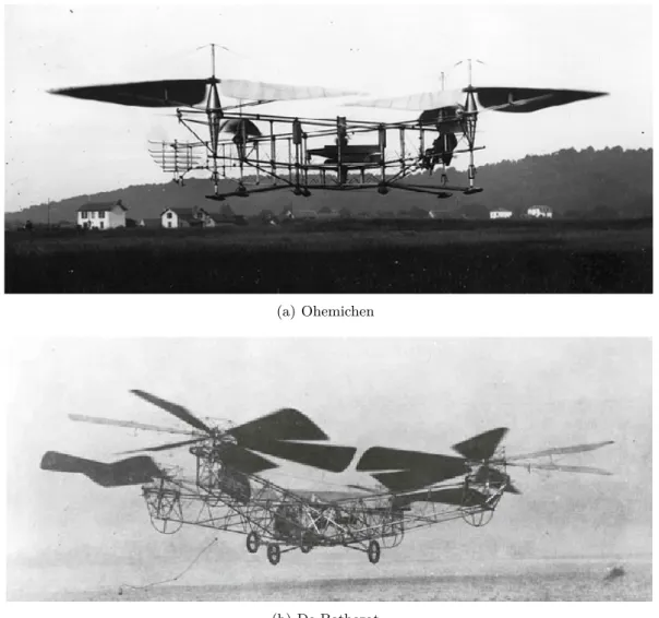
The first quadrotors were designed in the 20s as manned vehicles. The prototype known as Oehmichen N°2, created by the French engineer �tienne Oehmichen, was probably the first reliable VTOL (vertical take-off and landing) aircraft to be able to carry a person for at least one kilometer2_{. Another early experimental quadrotor}

was designed by George de Bothezat for the US army, but it had too many reliability and control problems, so the project was soon canceled [12]. This two prototypes are shown in Figure 1.

Nowadays, quadrotors are mainly employed as small scale UAVs for research and entertainment purposes. In the last few years some models were successfully introduced to the mainstream market, like the Parrot AR.Drone (Figure 2) which can be controlled from an iPhone and includes some predefined gaming apps. More relevant applications are surveillance and air photography and even the scouting of buildings, thanks to their indoor flying capability. As stated above, quadrotors are also often chosen by scholars and researchers as the reference platform for research in the fields of robotics, autonomous vehicles and flight control algorithms.

1 _{In traditional helicopters, the pitch of the main rotor blades can be adjusted either globally,} using the so called collective control to change the altitude or depending on the blade position, using the cyclic control, to change the direction of ﬂight.

2 _{The ﬁrst kilometer-long ﬂight took place in 1924 and lasted 7 minutes and 40 second.}

(19)

(a) Ohemichen

(b) De Bothezat

(20)

(21)

State of the art

Most of the research interest about vertical take off and landing UAVs is focused on the quadrotros. Some researchers developed their own platforms, such as the tiny Mesicopter [21], the X4-flier [14] or the one by Castillo [8], while other worked on commercially available models. The majority of the papers regards the development and evaluation of control algorithms. Many different control tecniques that have been proposed include:

• linear contollers (PID, PD) [4,36]; • Lyapunov theory [8,31];

• adaptive techniques [3,27]; • visual feedback [26,2]; • fuzzy algorithms [9]; • neural networks [11].

Other researches focus on the employs of this aerial vehicles, from multi-agent patrolling and surveillance [16, 10] to more fancy ones, like structure building [23] and river mapping [32].

The application of the extended Kalman filter to the quadrotors, which is the topic of this thesis, is also described in some papers. An attitude determination algorithm is proposed and tested by Liu and Zhou [24], while Abeywardena and Munasinghe [1] analyze the performance of another algorithm using a Matlab sim-ulation. The EKF is used to solve the state estimation problem in the works by Kis [20], Soumelidis [33] and Hoffmann [15], which are however more focused on the control system. Other researchers used the filter on visual informations to perform navigation tasks [25,35].

Structure of the thesis

The thesis is structured as follows:

Chapter 1 explains the basics of the extended Kalman ﬁlter and derives the dy-namic and sensor model of the quadrotor in a form that is suitable for the application of the ﬁlter.

Chapter 2 describes the Simulink model used to test the implementation of the EKF. The model extends a pre-existing one created by Tommaso Bresciani [6].

Chapter 3 analyzes the performance and the robustness of the Simulink EKF model by presenting data from various simulated test cases.

(22)

Appendix A provides the formal mathematical derivation of both the discrete and continuous time versions of the Kalman ﬁlter.

Appendix B contains all the Matlab code used by the Simulink model described Chapter 2.

(23)

Chapter 1

Attitude estimate with the

extended Kalman ﬁlter

The first section of this chapter provides a very concise introduction to the Kalman filter equations and implementation. A much more complete description of the filter theory with mathematical proofs can be found in Appendix A. Section 1.2 derives the dynamic equations that describe the quadrotor attitude and movements. In Section1.5the on board sensors are described. Finally, in Section 1.6the dynamic system and the sensor model are put in an appropriate form for the EKF to be applied and their linearizations are computed as required by the filter.

1.1 Introduction to Kalman ﬁltering

The original formulation of the Kalman filter was developed by Rudolf Emil Kálmán at the beginning of the ’60s [19, 18]. The filter algorithm assumes a discrete time linear dynamic system that can be represented as a difference equation using the state space model:

xk= Fkxk−1+ Bkuk−1+ wk, (1.1) where Fk is the state matrix, xk is the vector of the state variables, Bk is the input matrix, ukis the control vector and wkis a zero-mean, gaussian distributed process noise. If the system is time invariant, the matrices F and B do not depend on the time k. The ﬁlter also assumes the availability of a set of measurements that are also linear functions of the state variables:

zk= Hkxk+ vk, (1.2)

where H_kis the measurement matrix and v_kis also a zero-mean, gaussian distributed measurement noise uncorrelated with w_k

The Kalman ﬁlter is a recursive algorithm that exploits the knowledge of the expected covariance of the state variables to correct the a priori estimation of both the state of the system and the covariance itself. The estimate obtained by the

(24)

Kalman ﬁlter is statistically optimal. The algorithm can be divided in two main steps (in the following equations, a (_{−) after a variable indicates its estimated value} before the measurement update, while a (+) indicates the estimate after the update): Prediction step: at this step, the state at time k is predicted according to the

system model:

ˆ

xk(−) = Fk−1xˆk−1(+) + Bk−1uk−1. (1.3) The covariance at time k is also predicted according to the equation:

Pk(−) = Fk−1Pk−1(+)FkT−1+ Qk−1, (1.4) where Qk is the covariance of the process noise wk in Equation (1.1).

Update step: at this step, the a priori estimate is updated according to the mea-surements:

ˆ

xk(+) = ˆxk(−) + Kk[zk− Hkxˆk(−)] (1.5) and the covariance estimate is also updated:

Pk(+) = [I− KkHk]Pk(−). (1.6) The matrix Kk in Equations (1.5) and (1.6) is the optimal Kalman gain at time k, which is computed as:

Kk = Pk(−)HkT[HkPk(−)HkT + Rk]−1, (1.7) where R_k is the covariance of the measurement noise v_k in Equation 1.2. In practical applications, the error covariance matrices Q and R and the measure-ment matrix H are often time invariant.

1.1.1 Kalman ﬁlter for continuous time systems

A version of the Kalman filter known as the Kalman-Bucy filter can be applied to continuous time dynamic system. In this case, the system model is a differential equation:

˙

x = F (t)x(t) + B(t)u(t) + w(t) (1.8)

and the measurement model is also a continuous linear function of the state:

z(t) = H(t)x(t) + v(t). (1.9)

The main diﬀrerence with respect to the discrete time version is that in the continuous domain the update and the prediction steps are coupled and cannot be distinguished, so the ﬁlter consists of only two equations:

˙ˆ

x = F (x) ˆx(t) + B(t)u(t) + K(t)[z(t)− H(t)ˆx(t)], (1.10)

˙

(25)

and the Kalman gain is:

K(t) = P (t)HT(t)R−1. (1.12)

The equation (1.11) that expresses the covariance update is known as a Riccati equation1.

1.1.2 The extended Kalman ﬁlter

One of the main limitations of the Kalman filter is the fact that it requires both the dynamic system and the measurement functions to be linear with respect to the state variables. In many pratical applications, these requirements are not satisfied. The extended Kalman filter is a modified version of the standard Kalman filter that can be applied when the system and/or the measurement models are nonlinear.

Equation (1.13) and (1.14) are respectively the nonlinear diﬀerential (for the continuous case) and diﬀerence (for the discrete case) equations that describe the system model:

˙

x(t) = f (x(t), u(t)) + w(t), (1.13)

xk= Φk−1(xk−1, uk−1) + wk−1. (1.14) The nonlinear measurement model equation for the continuous and discrete time version are respectively:

z(t) = h(x(t)) + v(t), (1.15)

zk= hk(xk) + vk. (1.16) The nonlinear equations are used directly for the state prediction and to compute the measurement residual, so Equation (1.3), (1.5) and (1.10) become respectively:

ˆ xk(−) = Φk−1( ˆxk−1(+), uk−1), (1.17) ˆ xk(+) = ˆxk(−) + Kk[zk− hk( ˆxk(−))], (1.18) ˙ˆ x(t) = f ( ˆx(t), u(t)) + K(t)[z(t)− h(ˆx(t))]. (1.19)

The part concerning the covariance update is more complex. If the state transition and measurement equations are nonlinear, the probability distribution of the state vector becomes non-Gaussian, so it cannot be fully described by the mean and the covariance matrix alone. The EKF linearizes the state transition and measurement models around the current state estimate and it uses the Jacobians to update the covariance estimate with the same equations used by the standard Kalman filter. So in the discrete model we redefine Fkin Equation (1.4) and Hkin Equation (1.6) 1 _{A Riccati equation is any first order ordinary differential equation (in scalar or matrix form)} that is quadratic in the unknown function. It is named after the Italian matematician Jacopo Francesco Riccati (1676-1754).

(26)

and (1.7) as: Fk−1 =    ∂Φ1 ∂x1 · · · ∂Φ1 ∂xn .. . . .. ... ∂Φm ∂x1 · · · ∂Φm ∂xn    ˆ x_k−1(+),u_k−1 , Hk =    ∂h1 ∂x1 · · · ∂h1 ∂xn .. . . .. ... ∂hm ∂x1 · · · ∂hm ∂xn    ˆ xk(−) .

In the continuous model, we redeﬁne F (t) and H(t) in Equation (1.11) and (1.12) as: F (t) =    ∂f1 ∂x1 · · · ∂f1 ∂xn .. . . .. ... ∂fm ∂x1 · · · ∂fm ∂xn    ˆ x(t),u(t) ; H(t) =    ∂h1 ∂x1 · · · ∂h1 ∂xn .. . . .. ... ∂hm ∂x1 · · · ∂hm ∂xn    ˆ x(t) .

Since the Jacobians have to be evaluated at the current estimate in real time, the EKF is more complex than the standard Kalman ﬁlter from the computational point of view.

1.2 Quadrotor dynamics

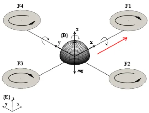
In order to provide the state-transition model to the extended Kalman filter, we need a physical model of the quadrotor dynamics and kinematics that is both accurate and simple enough to be mathematically analyzed and simulated on a computer system. The proposed model is shown in Figure1.2: the quadrotor is represented as a symmetric cross-like structure with a spherical central mass and four propellers, the front and the back ones rotate clockwise and the other two rotate counterclockwise. The mass of the structure that connects the propellers to the central mass is assumed negligible. The model is completed with the definition of two different Cartesian reference frames: the earth frame and the body frame, which are fully described in the following subsection.

1.2.1 Earth frame and body frames

As stated before, our dynamic model involves two diﬀerent reference frames: the earth frame is centered on a given point at ground level with the z_f axis pointing upwards, y_f pointing towards the magnetic north and x_f pointing to the east, while

(27)

Figure 1.1: Model of the quadrotor with two Cartesian reference frames. The red arrow indicates the main direction of motion.

the body frame is centered at the mass center of the aircraft, with the x_b axis directed towards the main direction of motion (which is usually arbitrary because of the symmetric structure of the quadrotor), the yb axis pointing to the left and the

zb axis pointing upwards with respect to the aircraft body. Both the frames follow the right hand convention.

Once we have deﬁned the two reference frames, we need a set of transformations between them, so that any vector given in the earth frame can be expressed in the body frame and vice-versa. These transformations are required because our goal is to control the attitude of the object with respect to the enviroment, but the measurements provided by the on-board sensors are referred to the body frame. While the translations are quite straightforward and actually they are not even really important for our purposes (an active control of the position is not developed in this thesis), the three dimensional rotations are much more complex than their two-dimensional counterpart, so a complete explanation is needed.

1.2.2 Euler angles

The Euler angles are one way to describe the orientation of a rigid body with respect to a ﬁxed reference frame. They were introduced by Leonhard Euler in the 18th century, but are still widely used. The Euler angles can be explaind using the rotations around the moving axes, known as intrinsec rotations, that are simple to imagine: if we at ﬁrst rotate the frame around the x axis, then the y axis will end up

(28)

pointing in a diﬀerent direction than the initial one. A second rotation around the y axis will rotate the frame around this new direction. In general, each new rotation is referred to the direction that its axis has assumed after all the previous ones.

Given two cartesian reference frames with the same origin, the first frame can be rotated to match the orientation of the second frame by applying three rotations around the moving axes in a given order. The sequence of the three rotations uniquely defines the orientation of the second reference frame with respect to the first one. To avoid ambiguity, the chosen sequence of rotation axes must follow a common convention. We will use the sequence z− y − x, which is conventional in aerospace engineering. The resulting angles ψ, θ and φ are called respectively yaw,

roll and pitch2_.

Rotation matrix

The rotations around the three axes of a Cartesian frame are analitically described by the following matrices:

R(x, φ) =  10 cos φ0 _{− sin φ}0 0 sin φ cos φ   , R(y, θ) =   cos θ0 01 sin θ0 − sin θ 0 cos θ   , R(z, ψ) = 

cos ψsin ψ − sin ψ 0cos ψ 0

0 0 1

  .

It is important to notice that we have described the Euler angles using the rotations around the moving axis, because they are easier to understand by intuition, but the above matrices perform the rotations around the axes of the ﬁxed reference frame (called extrinsic rotations). However, it is possibile to prove that any sequence of intrinsic rotations is equivalent to the same sequence of extrinsec rotations performed in reverse order, in our case x− y − z is the opposite of z − y − x (that’s also the reason why the Euler angles are usually listed as roll, pitch and yaw and not the other way around as we did in the previous paragraph). So, the full rotation matrix is computed in the following way3:

2 _{The angles deﬁned according to this convention are more properly called Tait-Benn angles,} because the original Euler angles perform the ﬁrst and the last rotations around the same axis.

3_{Remember that the matrix product is not commutative and the ﬁrst rotation is associated to} the leftmost matrix.

(29)

R(φ, θ, ψ) = R(z, ψ)R(y, θ)R(x, φ) = =



cos ψ cos θ cos ψ sin θ sin φsin ψ cos θ sin ψ sin θ sin φ + cos ψ cos φ sin ψ sin θ cos φ− sin ψ cos φ cos ψ sin θ cos φ + sin ψ sin φ_{− cos ψ sin φ}

− sin θ cos θ sin φ cos θ cos φ

  . (1.20) The matrix R(φ, θ, ψ) and its inverse (which corresponds to its transpose because it is an orthogonal matrix) can be used to switch between the body frame and the earth frame: if x is a vector in the body frame, Rx expresses the same vector in the earth frame, on the contrary, a vector y deﬁned in the earth frame becomes RT_y in the body frame.

Geometric deﬁnition of the Euler angles

In the previous paragraphs we have deﬁned the Euler angles in the Cartesian space by an operative deﬁnition, decribing how to move one frame to make it conincident with the second one, and in an analitic way, explaining how to obtain the body frame by transforming the coordinates of the earth frame. However, the angles φ, θ and

ψ can also be described by a geometric definition, as shown in Figure 1.2.2. First of all, we define the line of nodes as the interception between the earth frame xfyf plane and the body frame y_bzb plane4. Then, according to our previous convention, the Euler angles are defined as follows:

• φ is the angle between y_b and the line of nodes;

• θ is the angle between x_b and its projection on the y_fyf plane; • ψ is the angle between y_f and the line of nodes.

1.2.3 Angular velocities

Now we can use the Euler angles to express the angular velocity, which is deﬁned as:

ω = dθ

dtu (1.21)

where θ is the rotation angle and u is the versor oriented in the direction of the rotation axis. If ω is the angular velocity of the quadrotor, it can be decomposed along three directions: the line of nodes, the zf axis and the xb axis:

ω = ωn+ ωzf + ωxb. (1.22)

4_{According to this deﬁnition, the line of nodes is undeﬁned when θ =}_{±90°. In this case, two} of the three rotation axes become coincident and the system loses one degree of freedom. This is a well-known problem of the Euler angles called the gimbal lock.

(30)

Figure 1.2: Visual representation of the Euler angles

These three directions are not an orthogonal basis, but it is convenient to use them because they are the rotation axes of the Euler angles that we have just deﬁned, so we can write:

ω = ˙φxb+ ˙θn + ˙ψzf. (1.23)

Finally, we can ﬁnd the angular velocity with respect to the body frame by trans-forming the versors zf and n with the matrix RT:

RTzf = RT  00 1   = 

cos θ sin φ− sin θ cos θ cos φ   , (1.24) RTn = RT  _{− sin ψ}0 cos ψ   =   cos φ0 − sin φ   , (1.25)

ω = ( ˙φ− ˙ψ sin θ)xb+ ( ˙θ cos φ + ˙ψ cos θ sin φ)yb+ (− ˙θ sin φ + ˙ψ cos θ cos ϕ)zb. (1.26) The latter equation can be written in matrix form:

ωB =  pq r   = RR(φ, θ, ψ)  φ_θ˙˙ ˙ ψ   with: RR(φ, θ, ψ) = 

10 cos φ0 sin φ cos θ− sin θ 0 − sin φ cos φ cos θ 

(31)

In practice, since the sensors on the quadrotor directly measure the values of

p, q and r, the inverse of RR is much more useful. First of all, we note that det(R_R) = cos θ, so the matrix becomes singular for θ = ±90° (a consequence of the gimbal lock). For θ̸= ±90° the matrix is invertible and its inverse is:

RR(φ, θ, ψ)−1= 

10 sin φ tan θ cos φ tan θcos φ − sin φ 0 sin φ_{cos θ} cos φ_{cos θ}



 . (1.28)

1.3 Rigid body dynamics

The dynamic equations for the quadrotor are usually formulated in the body frame rather than in the earth frame, because of some reasons:

• the inertia matrix is time-invariant;

• body symmetry can be exploited to simplify the equations;

• sensor measurements and driving forces are naturally expressed in the body frame.

1.3.1 Linear motion

The well known Newton’s second law states that:

mdv

dt = F (1.29)

where F is the total force acting on the body center of mass.

Since Newton’s laws are valid only for inertial systems, we cannot directly apply Equation (1.29) to the body frame. If we have a moving vector inside a reference frame which, in turn, rotates with respect to a ﬁxed frame, we can apply the equation of Coriolis to relate the derivative of the vector in the body frame (dv

dt )

b to its derivative in the inertial frame(dv

dt ) i: ( dv dt ) i = ( dv dt ) b + ω_b/i× vb, (1.30)

where ω_b/iis the angular velocity of the moving frame with respect to the ﬁxed one. Combining Equations (1.29) and (1.30) we can write:

m(v˙b+ ωb/i× vb ) = F , and then: ˙ vb=−ωb/i× vb+ F m. (1.31)

(32)

1.3.2 Angular motion

Newton’s second law for the angular acceleration has the following form:

dh

dt = τ , (1.32)

where h is the angular momentum of the rigid body and τ is the applied torque. We can obtain its expression in the body frame using the same Equation (1.30) that we used for the linear acceleration:

˙

hb=−ω × hb+ τ (1.33) and then, since the angular momentum is the angular velocity multiplied by the time-invariant inertia matrix J :

J ˙ω =−ω × Jω + τ , (1.34) with ω = [p, q, r]T_.

The moment of inertia tensor

The moment of inertia tensor for a rigid body is a positive semideﬁnite symmetric matrix: J =  JJXXXY JJXYY Y JJXZY Z JXZ JY Z JZZ   . (1.35)

As stated before, the quadrotor can be modeled as a central sphere of mass M and radius R connected with four point masses m at distance l from the center (representing the motors). According to this model, the quadrotor is symmetrical about the three axes, so J becomes a diagonal matrix with:

JXY = JXZ = JY Z = 0, JXX = JY Y = 2M R2 5 + 2ml 2_, JZZ = 2M R2 5 + 4ml 2_. 1.3.3 Altitude

An attitude control system does not perform navigation tasks, so the estimation of the linear position with respect to the earth frame is not needed. However the vertical component z must be taken into account, because the system should avoid unwanted and potentially dangerous altitude variations while manouvering. The derivative of z is the vertical component of the velocity vector with respect to the body frame, which can be computed from the body frame velocity values using the matrix (1.28):

˙

(33)

1.4 Forces and controls

The only variable that we can directly control to aﬀect the motion of the quadrotor is the speed of each propeller, so we have to relate their values to the torques τx, τy and τz, which are the control variables described later in Equation (1.61). For most ﬂight conditions of practical interest, it can be proven that each motor generates a force that is proportional to the square of its angular speed and perpendicular to the rotor plane: Fi = bΩ2i, where b is a constant. Thus the total force acting on the quadrotor is always directed upwards with respect to the body frame and its modulus is:

F = Fr+ Fl+ Ff + Fb = b(Ω2r+ Ω2l + Ω2f + Ω2b). (1.37) This force, combined with the proper roll and pitch angles, can be used to move the quadrotor in any direction.

The rolling torque is the result of the diﬀerence between the forces of the left and the right motors and the pitching torque is produced in the same way by the diﬀerence between the forces of the front and the back motors:

τφ= l(Fl− Fr) = bl(Ω2l − Ω2r), (1.38)

τθ= l(Ff− Fb) = bl(Ω2f − Ω2b). (1.39) In these two equations, l is the distance between the rotors and the mass centre of the quadcopter. The yawing torque is generated by a diﬀerent principle: according to Newton’s third law, each rotor produces a yawing torque on the body of the quadrotor in the opposite direction of the blades rotation, proportional to the square of the angular speed: τi = dΩ2_i. The total yawing torque is then the sum of the contributions of the single rotors5_:

τψ = τr+ τl− τf − τb = d(Ωr2+ Ω2l − Ω2f − Ω2b). (1.40) To be more accurate, the rotors, like every rotating object, are subject to the gyroscopic eﬀect. This implies that a torque perpendicular to the rotating plane generates a precession movement perpendicular to both the rotating plane and the torque. According to this principle, a pitch torque produces a roll and vice versa, so the equations (1.38) and (1.39) become:

τφ = bl(Ω2l − Ω2r) + Jmq(Ωf + Ωb− Ωl− Ωr), (1.41)

τθ= bl(Ω2f − Ω2b) + Jmp(Ωl+ Ωr− Ωf − Ωb) (1.42) where Jm is the inertia of the motor. In these equations, the term due to the gyroscopic eﬀect is proportional to the diﬀerence between the speed of the motors rotating clockwise and the ones rotating counter clockwise, because they generate 5_{The following equation is true if we assume that the left and right rotors rotate clockwise and} the front and back ones rotate counterclockwise, otherwise the signs are reversed.

(34)

two opposite torques that cancel out. This term is diﬀerent from zero only when the quadrotor is both yawing and rolling or pitching at the same time and even in that case it is very small with respect to the other term of the equation, so the gyroscopic eﬀect is often negected for pratical applications.

Now we can choose the control variables to make the dynamic equations linear with respect to them. The most natural choice is:

U1= b(Ω2f + Ω2b + Ω2l + Ω2r),

U2= bl(Ω2l − Ω2r),

U3= bl(Ω2f − Ω2b),

U4= bl(Ω2r+ Ω2l − Ω2f − Ω2b). If we write the previous equations in matrix form we obtain:

U = AΩsq=     b b b b 0 −bl 0 bl −bl 0 bl 0 −bl bl −bl bl         Ω2_b Ω2_r Ω2_f Ω2_l     . (1.43)

Since matrix A is invertible, each control variable Ui can assume any value inde-pendently from the others. Given the desired values of the control variables, the angular speeds required to obtain them can be computed as:

               Ωb = √ 1 4bU1− 1 2blU3− 1 4dU4 Ωr = √ 1 4bU1− 1 2blU2+ 1 4dU4 Ωf = √ 1 4bU1+ 1 2blU3− 1 4dU4 Ωl = √ 1 4bU1+ 1 2blU2+ 1 4dU4 . (1.44)

A problem arises if the quantities under the square roots are negative. In that case we would have imaginary values of Ω, which obviously have no physical meaning, thus the desired control is not achievable6_.

1.5 On board sensors

Every aircraft has a set of sensors that provide the information needed by the at-titude and the navigation control systems. This set of sensors is usually called an IMU (inertial measurement unit). The IMU of a quadrotor contains the following sensors:

6_{Actually, the rotor speed values of a real quadrotor are limited to some interval, so even besides} the imaginary case there is a big set of controls that are theoretically possibile, but cannot be achieved in pratice. Some dedicated control system has to be implemented to handle this problem.

(35)

• an accelerometer; • a gyroscope; • a magnetometer; • a barometer7_.

A typical three-axis MEMS sensor is calibrated according to this linear model:  yyxy yz   =  M1yx M1xy MMxzyz Mzx Mzy 1      1 Sx 0 0 0 _S1 y 0 0 0 _S1 z     xxxy xz   +  bbxy bz   +  vvxy vz   . (1.45) The variables used in the above equation are:

• xi: input value along the i-th axis; • yi: sensor output for the i-th axis; • bi: sensor bias on the i-th axis;

• vi: gaussian distributed random error on the i-th axis; • S_i: scale factor of the ith axis;

• Mij: sensitivity of the ith axis output to jth axis input.

In particular, the coefficients M_ij and the scale factors S_ireflect the fact that the axes of these low cost sensors are not perfectly aligned and their sensitivity differs from the nominal one. All the parameters vary with the temperature, but are assumed to be constant during the flight time of the quadrotor so a dynamic calibration is not required.

1.5.1 Gyroscope

The gyroscope measures the angular rates around the three axes. Its sensor model is a simple application of Equation (1.45):

yg= MgSgω + bg+ vg (1.46) where ω = [p, q, r]T_.

7 _{The barometer is used only to control the altitude and it is not a typical part of an IMU, so} it may be considered as an independet sensor.

(36)

1.5.2 Accelerometer

The accelerometer measures a quantity called proper acceleration along the three axes. The proper acceleration is the sum of the linear acceleration (the derivative of the linear velocity) and a constant pseudo-acceleration directed upwards with respect to the body frame that has the same magnitude as the gravity vector g8. If a is the proper acceleration vector in the body frame, from Equation (1.45) we have:

ya = MaSaa + ba+ va. (1.47)

Following the deﬁnition of proper acceleration, the components of the vector a can be written as: _

aaxy az   =  u˙˙v ˙ w   + 

_{−g cos θ sin φ}g sin θ

−g cos θ cos φ



 , (1.48)

where ˙u, ˙v and ˙w are the time derivatives of the linear velocity vector. Substituting

in Equation (1.47) we have: ya = MaSa    u˙˙v ˙ w   + 

_{−g cos θ sin φ}g sin θ

−g cos θ cos φ     + ba+ va. (1.49) 1.5.3 Magnetometer

A magnetometer is a sensor that measures the intensity and the direction of a magnetic ﬁeld. If the earth magnetic ﬁeld vector is known, the sensor output can be used to estimate the attitude of the quadrotor. According to Equation (1.45), in absence of magnetic distortions, the output of the magnetometer is:

ym = MmSmmb+ bm+ vm, (1.50) where mb is the magnetic ﬁeld vector with respect to the body frame, S and M are the matrices of scale and misalignment factors, bs is the sensor bias and vk is a random gaussian white noise.

Hard and soft iron distortions

Hard and soft iron distortions are caused by magnetic ﬁelds and metallic objects surrounding the sensor. If the sources of the distortions are parts of the quadrotor or its payload (motors, battery...), the distortions can be measured and corrected statically [28].

(37)

Hard iron distortions The hard iron distortions are caused by objects that pro-duce a magnetic ﬁeld. These distortions intropro-duce a ﬁxed bias in the measurements, so Equation (1.50) needs to be corrected by adding the bias vector h_h:

ym = MmSmmb+ bs+ hh+ vm. (1.51) Soft iron distortions The soft iron distortions are caused by ferromagnetic ma-terials surrounding the sensor. These distortions are more complex to model than the hard iron ones, because they depend upon the direction of the magnetic ﬁeld with respect to the sensor. To be more precise, let the sensor freely rotate in the space and let S be the set of all the possible values that the measured magnetic ﬁeld can assume. In absence of distortions, S is the surface of a sphere, because the measured vector can assume any direction, but its module does not change. The soft iron distortions apply a linear transformation to the measurement space, changing

S into an ellipsoid. A linear transformation in a tridimensional space is deﬁned by

a 3-by-3 matrix, so the sensor model becomes:

ym = HsMmSmmb+ bs+ hh+ vm. (1.52) However, we can sum the two bias vector and consider them as a single bias bm and multiply the matrices Hsand Mm to obtain a single transformation matrix G. This way, the espression for the sensor model becomes very similar to the standard Equation (1.45), except for the diagonal elements of G, which here can be diﬀerent from 1.

Since we want to use the sensor to determine the attitude of the quadrotor, it is useful to express the magnetic filed vector in body frame mb as a function of the euler angles φ, θ and ψ by using the inverse of the matrix R(φ, θψ) defined in Equation (1.20): if m_f is the magnetic field vector measured in the fixed frame we have:

mb= RT(φ, θ, ψ)mf, so Equation (1.52) becomes:

ym = GRT(φ, θ, ψ)mf + bm+ vm. (1.53)

1.5.4 Barometer

The barometer is different from the other sensors that we have described, because it measures a scalar value, so the model in Equation (1.45) cannot be applied. We want to use the barometer as an altimeter, so the instrument needs to know the current value of the pressure at the ground level (or another reference altitude). A static calibration is not possibile, because the ground pressure changes with weather conditions. In practice, the pressure is measured before the take off and assumed to be constant during the flight time. The pressure P and the altitude z are related by this formula:

P = P0e−

g

(38)

where P0 is the pressure at the known altitude z0 (usually the ground), g is the

gravitational acceleration, R is the dry air gas constant and T is the temperature at the altitude z9_{. Since the quadrotor is expected to ﬂy no higher that a few tenths}

of meters, we can assume T to be a constant, equal to the value T0 measured on the

ground.

The sensor model used for the barometer is:

yb= kbxb+ bb+ vb. (1.55) Combining the latter with Equation (1.54) and imposing z0= 0 we obtain the output

of the sensor as a function of the altitude z:

ya= kaP0e−

g

RTz+ b_a+ v_a. (1.56)

1.6 State space representation for the EKF

In the previous sections we have provided a matemathical description of the quadro-tor dynamics and controls and the operating principles of its sensors. Now we want to rearrange these equations in a form that is suitable for the application of the continuous time EKF. At ﬁrst, we have to identify the system variables, which are the variables that appear in the dynamic equations:

• u, v, w, the linear velocity components along the three axes of the body frame; • p, q, r, the angular velocitiy components around the three axes of the body

frame;

• φ, θ and ψ, the Euler angles roll, pitch and yaw (in this order); • z, the altitude of the quadrotor.

Therefore, we have to express both the state-transition model and the sensor model according to this set of 10 variables.

1.6.1 State-transition model

The general state-transition model for the continuous time EKF is described by the equation (1.8).

9_{A more accurate version of the equation (}_1.54_{) should take into account the relative humidity.} Note also that the assumption that P0 is constant is always true only for short periods of time, because weather changes cause signiﬁcant long-term pressure variations.

(39)

Linear velocity

The cross product in Equation (1.31) can be expressed in matrix form as:

ω× vb= [ω]_×vb=  _−r0 r0 −qp q −p 0    uv w   , (1.57)

where [_·]_× is the skew operator. We have to take into account also the gravitational force, which generates a ﬁxed acceleration of modulus g always directed downwards with respect to the earth frame. The equation ﬁnally becomes:

 u˙˙v ˙ w   =  _−r0 r0 −qp q −p 0    uv w   + 

_{−g cos θ sin ϕ}g sin θ

−g cos θ sin ϕ   + 1 m  FFxy Fz   (1.58) =  pwrv− qw− ru qu− pv   + 

_{−g cos θ sin ϕ}g sin θ

−g cos θ sin ϕ   + 1 m  FFxy Fz   . (1.59) Angular velocity

We can rewrite the equation (1.34) to explicit the derivatives of the angular velocity components:  pq˙˙ ˙r   =  J −1 XX 0 0 0 J_{Y Y}−1 0 0 0 J_ZZ−1      _−r0 0r −qp q −p 0    JXX0 JY Y0 00 0 0 JZZ    pq r   +  ττφθ τψ     (1.60) =    JY Y−JZZ JXX qr JZZ−JXX JY Y pr JXX−JY Y JZZ pq    +  J −1 XXτφ J_{Y Y}−1τθ J_ZZ−1τψ   . (1.61) Euler angles

We do not have a dynamic equation that involves the derivatives of the Euler angles, but we have used them to deﬁne the angular velocity with respect to the body frame, so we can use the matrix R_R(φ, θ, ψ)−1in Equation (1.28) to express the derivatives of φ, θ and ψ as functions of the angular velocity components p, q and r:

     ˙

φ = p + sin ϕ tan θq + cos ϕ tan θr

˙

θ = cos φq− sin φr

˙

ψ = sin φ_{cos θ}q +cos φ_{cos θ}r

(40)

Complete model

We can now write the complete state-transition model by combining Equations (1.59), (1.61), (1.62) and (1.36):                                          ˙ u = rv− qw + g sin θ ˙v = pw− ru − g cos θ sin φ ˙ w = qu− pv − g cos θ cos φ + U1_m ˙ p =IY Y−IZZ IXX qr + 1 IXXU2− Jm IXXqΩR ˙ q = IZZ−IXX IY Y pr + 1 IY YU3+ Jm IY YpΩR ˙r = IXX−Iyy IZZ pq + 1 IZZU4 ˙

φ = p + sin φ tan θq + cos φ tan θr

˙

θ = cos φq− sin φr

˙

ψ =sin φ_{cos θ}q + cos φ_{cos θ}r

˙

z =− sin θu + cos θ sin φv + cos θ cos ϕw

(1.63)

where ΩR= Ωl+ Ωr− Ωf − Ωb.

1.6.2 Measurement model

The general measurement model for the EKF is described by Equation (1.9). We have to express all the sensor equations as functions of the state variables.

Accelerometer

While the equations for the gyroscope, the magnetometer and the barometer de-ﬁned in Section 1.5are already functions of the state variables, the equation of the accelerometer (1.49) is a function of the derivative of the linear velocity. However, we can substitute ˙u, ˙v and ˙w for their expressions in the dynamic equation (1.31):

ya = MaSa     pwrv− qw− ru qu− pv + U1_m   + ba+ va   , (1.64)

which is a function of the state variables. It is important to note that this equation contains also the control variable U₁. In the standard EKF measurement model, the control variables are not involved, but the ﬁlter should still work without modiﬁca-tions as long as the value of the variable is known without uncertainty. In any case, this particular situation must be taken into account during the implementation.

(41)

Complete model

The complete measurement model can be obtained by combining Equations (1.64), (1.50), (1.46) and (1.56):                      ya= MaSa    rv− qw pw− ru qu− pv + U1_m    + ba+ va yg= MgSgω + bg+ vg ym= GRT(φ, θ, ψ)mf + bm+ vm yb = kbP0e− g RTz+ b_b+ v_b . (1.65) 1.6.3 Linearizations

As we said in Subsection1.1.2, the extended Kalman ﬁlter requires both the state-transition and the measurement models to be linearized using the Jacobians. Jacobian of the state-transition model

If we ignore the gyroscope eﬀect, which is almost always negligible, the Jacobian of the state-transition model is a 10-by-10 sparse matrix10. Its nonzero elements are:

J1,2= r; J1,3=−q; J1,5=−w; J1,6= v; J1,8= g cos θ; J2,1=−r; J2,3= p; J2,4= w; J2,6=−u; J2,7=−g cos θ cos φ; J2,8= g sin θ sin φ; J3,1= q; J3,2=−p; J3,4=−v; J3,5= u; J3,7= g cos θ sin φ;

10_{A matrix is sparse if more than an half of its elements are zeros. In this case, 60 of the 100} elements are zeros.

(42)

J3,8 = g sin θ cos φ; J4,5 = IY Y − IZZ IXX r; J4,6 = IY Y − IZZ IXX q; J5,4 = IZZ− IXX IY Y r; J5,6 = IZZ− IXX IY Y p; J6,4 = IXX− IY Y IZZ q; J6,5 = IXX− IY Y IZZ p; J7,4 = 1; J7,5 = sin φ tan θ; J7,6 = cos φ tan θ;

J7,7 = cos φ tan θq− sin φ cos θr;

J7,8 = sin φq + cos φr cos2_θ ; J8,5 = cos φ; J8,6 =− sin φ; J8,7 =− cos φr − sin φq; J9,5 = sin φ cos θ; J9,6 = cos φ cos θ; J9,7 = cos φq_{− sin φr} cos θ ; J9,8 = tan θ

cos θ(sin φr + cos φq); J10,1=− sin θ;

J10,2= cos θ sin φ;

J10,3= cos θ cos φ;

J10,7= cos θ cos φv− cos θ sin φw;

(43)

Jacobian of the measurement model

The jacobian of the sensor model is also a sparse matrix of the form:

J =     J1 J2 03×4 03×3 MgSg 03×4 03×3 03×3 Jm 0 01×9 Ja     . (1.66)

The submatrices that compose the above matrix are:

• J₁: the derivatives of the accelerometer equation with respect to the linear velocity variables u, v, w;

• J₂: the derivatives of the accelerometer equation with respect to the angular velocity variables p, q and r;

• J3: the derivatives of the magnetometer equation with respect to the euler

angle variables φ, θ and ψ;

• Ja(scalar): the derivative of the altimeter equation with respect to the altitude variable.

Their expressions are:

J1= MaSa  _−r0 r0 −qp q −p 0   ; (1.67) J2= MaSa  w0 −w0 −uv −v u 0   ; (1.68) J3= [ G∂RT(φ_∂φ0,θ0,ψ0)mf G∂R T_(φ_0,θ0,ψ0₎ ∂θ mf G ∂RT(φ0,θ0,ψ0) ∂ψ mf ] ; (1.69) Ja=− kaP0g RT e − g RTz. (1.70)

(44)

(45)

Chapter 2

Simulation model

This chapter contains the description of the Simulink model developed to test the performance of the attitude control system based on the extended Kalman ﬁlter. Our work actually extends a pre-existing model developed by Tommaso Bresciani for his master thesis.

The ﬁrst section of this chapter describes the pre-existing model, Section 2.2.1 regards the model of the on board sensors (which was missing in the model by Bresciani) and ﬁnally Section2.3describes the model of the EKF both in continuous and discrete time.

The simulink models of the system and its blocks are shown here, while the Matlab code used to implement some blocks is listed in AppendixB.

2.1 Pre-existing model

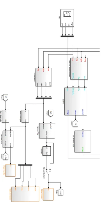
The higher-level structure of the pre-existing model is shown in Figure 2.1. The main signals that connect the blocks are:

pos-vel-acc: this signal groups together the information about the linear and an-gular position, velocity and acceleration of the aircraft, so it is actually a mux of 8 vector signals, each one of which has three components.

omega: this signal is a vector of four components that represent the angular rates of the propellers.

Vcontrol: this signal is a vector of four components that represent the current voltages generated by the control to power the engines.

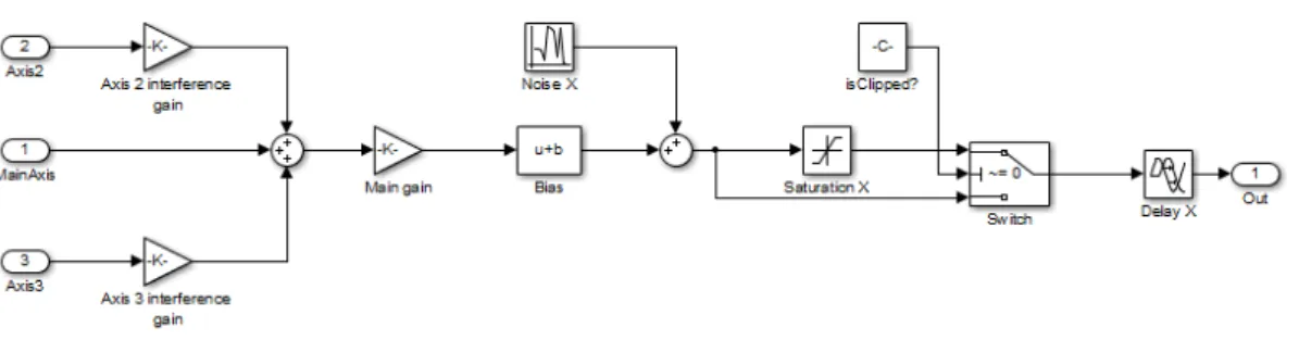
target: this signal is generated by the user and contains the information about the desired behaviour of the quadrotor. It has four components: roll, pitch, yaw and altitude.

(46)