View of Some considerations and developments about recently proposed families of distributions with hinge points

SOME CONSIDERATIONS AND DEVELOPMENTS ABOUT RECENTLY PROPOSED FAMILIES OF DISTRIBUTIONS WITH HINGE POINTS

Maurizio Brizzi

1. INTRODUCTION

The research work regarding probability density models is, necessarily, always in progress, since many researchers are interested in finding reasonably simple functions, which are able to fit a set of experimental data. Nowadays, we receive a lot of quantitative information concerning several fields, from biology to sociol-ogy, from chemistry to economy, from sport to music, and the list would be much longer; therefore, we often have to deal with “new” sets of data, and is al-ways more important to have a large choice of probability models, discrete or continuous, in order to find the best fitting one.

Sometimes, when representing the distribution of some kind of natural or so-cial phenomena, we realize that smaller values have a different behaviour than larger ones, so that we cannot use an unique type of function, but rather two (or more) different functions, separated by hinge points.

In this paper, two families of p.d.f.’s with hinge points are discussed and de-veloped. The first one is the MTSP (Modified Two-Sided Power), derived from the STSP (Standard Two-Sided Power), defined and studied by Van Dorp and Kotz (2002a); the second one is the two-faced distribution (TF), recently pro-posed in Brizzi (2006), defined by joining a triangular distribution and an expo-nential one.

2. FROM STSP TO MTSP

The Standard Two-Sided Power distribution is a limited domain model, de-pending on two parameters: the “hinge point” θ, in which the p.d.f. changes and becomes to decrease, and the shape parameter κ. In its original proposal by Van Dorp and Kotz (2002), the domain is the interval [0,1], and the p.d.f. is the fol-lowing:

1 1 0 ( ) 1 ₁ 1 X x x f x x _x κ κ κ θ θ κ θ θ − − ⎧ _{⎛ ⎞} < ≤ ⎪ ⎜ ⎟ ⎪ ⎝ ⎠ = ⎨ − ⎪ ⎛ ⎞ _{< ≤} ⎜ ⎟ ⎪ _{⎝ − ⎠} ⎩ (1)

The effect of varying the parameters is represented in Figure 1 (where θ is fixed and κ is variable) and Figure 2 (κ fixed and θ variable).

Figure 1 – Probability density function of some STSP distributions (θ = 0.4,κvariable).

Figure 2 – Probability density function of some STSP distributions (κ = 3, θ variable).

The MTSP distribution family is generated by modifying the central part of an STSP distribution. The basic idea is to “strengthen” the neighbourhood of the hinge point θ by adding an uniform component.

( ) (1 ) ( ) ( )

Y Y U

f y = −α f y +α f y (2)

where X is a STSP (κ, θ) and U is an Uniform (θ−β/2, θ+β/2). The domain of Y is the interval [0,1], the same of STSP distribution.

The p.d.f. assumes, within its domain, four different expressions:

1 y /2 , 1 1 ) 1 ( /2 y , 1 1 ) 1 ( y /2 , ) 1 ( /2 -y 0 , ) 1 ( ) ( 1 1 1 1 ⎪ ⎪ ⎪ ⎪ ⎪ ⎩ ⎪ ⎪ ⎪ ⎪ ⎪ ⎨ ⎧ ≤ < + ⎟ ⎠ ⎞ ⎜ ⎝ ⎛ − − − + ≤ < + ⎟ ⎠ ⎞ ⎜ ⎝ ⎛ − − − ≤ < + ⎟ ⎠ ⎞ ⎜ ⎝ ⎛ − ≤ < ⎟ ⎠ ⎞ ⎜ ⎝ ⎛ − = − − − − β θ θ κ α β θ θ β α θ κ α θ β θ β α θ κ α β θ θ κ α κ κ κ κ y y y y y fY (3)

Parameters and corresponding parametric spaces are listed below:

α = Weight of the uniform component 0 <α < 1

β = Width of the uniform component 0 < β < 2 min [θ, (1–θ)]

κ = Shape parameter κ > 0

θ = Mode and hinge point 0 <θ < 1

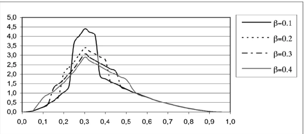
In Figures 3 and 4 we have represented the p.d.f. of a MTSP distribution, as a function of the parameters α, β.

Figure 4 – Probability density function of some MTSP distributions (κ=0.3,θ=0.3, α=0.2, β vari-able).

The cumulative distribution function FY(y) assumes, within its domain [0, 1], four

different expressions (outside the domain, the c.d.f. is obviously constant, 0 on the left and 1 on the right):

(1 ) , 0 y - /2 ( /2) (1 ) , - /2 y ( ) 1 ( /2) (1 ) 1-(1- ) , y /2 1 1 (1 ) 1-(1- ) , /2 y 1 1 Y y y y F y y y y κ κ κ κ α θ θ β θ θ β α θ α θ β θ θ β θ β α θ α θ θ β θ β α θ θ β θ ⎧ _{⎛ ⎞} − < ≤ ⎪ ⎜ ⎟ ⎝ ⎠ ⎪ ⎪ _{⎛ ⎞ − −} ⎪ − _{⎜ ⎟} + < ≤ ⎪ ⎝ ⎠ ⎪ =⎨ _{⎡ − ⎤ − −} ⎛ ⎞ ⎪ − ⎢ ⎜ ⎟ ⎥+ < ≤ + ⎪ ⎢_⎣ ⎝ − ⎠ ⎥_⎦ ⎪ ⎪ ⎡ _{⎛ − ⎞} ⎤ − + < ≤ ⎪ ⎢ ⎜ ₋ ⎟ ⎥ ⎝ ⎠ ⎢ ⎥ ⎣ ⎦ ⎩⎪ (4)

In particular, we have, at point θ:

Y X U

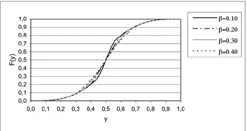
F ( ) (1- ) F ( )θ = α θ + α F ( ) (1- )θ = α θ α+ / 2= +θ α(1/ 2−θ) (5) In Figure 5 and Figure 6 the c.d.f. of MTSP distribution is represented, as a

Figure 5 – Cumulative distribution function of MTSP (αvariable, β=0.20 ).

Figure 6 – MTSP cumulative distribution function (α=0.20, β variable). The expected value of a MTSP distribution is:

( 1) 1 (2 1) 1 E( )=(1 ) E(X) E( ) (1 ) 1 1 Y α α U α κ θ αθ α κ θ α κ κ − + + − + − − + = − + = + + (6)

Therefore, E(Y) does not depend on β. When α increases, E(Y) moves linearly towards θ. For example, fixing some values of θ and κ, we may derive, by chang-ing the value of α, the expected values represented in Table 1:

TABLE 1

Expected value of MTSP as a function of α

The effect of increasing α is to move the expected value towards the value of

θ, which is the central point of the uniform window; when θ=1/2, there is no effect, since we have already E(X) =θ. The effect of increasing α is to move the expected value towards the value of θ, which is the central point of the uniform window; when θ=1/2, there is no effect, since we have already E(X) =θ.

The second moment of Y, i.e. the expected value of Y2 _{, is:}

2 2 2 ( ) (1 ) ( ) ( ) E Y = −α E X +α E U = _{(1 )} 3 _{(1 ) 2 (1 )}2 _{(1 )}3 2 2 ( 2) 1 2 12 κθ κ κ β α θ θ θ α θ κ κ κ ⎡ ⎤ ⎛ ⎞ = − _⎢ + − − − + − _⎥+ _⎜ + _⎟ + + + ⎣ ⎦ ⎝ ⎠ (7)

Consequently, the variance V(Y)=E(Y2_)-[E(Y)] 2 _{assumes a troubling}

compli-cated general expression. Nevertheless, we can study the effect of varying α and

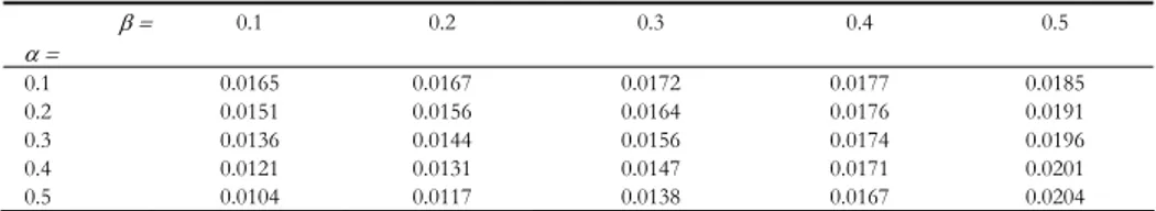
β by fixing the values of the STSP parameters, κ and θ. We have reported, in Ta-ble 2, the variance corresponding to some values of α and β for κ = 4 and θ =1/3.

TABLE 2 Variance of MTSP for κ = 4 , θ = 1/3 β = 0.1 0.2 0.3 0.4 0.5 α = 0.1 0.0165 0.0167 0.0172 0.0177 0.0185 0.2 0.0151 0.0156 0.0164 0.0176 0.0191 0.3 0.0136 0.0144 0.0156 0.0174 0.0196 0.4 0.0121 0.0131 0.0147 0.0171 0.0201 0.5 0.0104 0.0117 0.0138 0.0167 0.0204

The effect of varying β becomes stronger as well as α increases; on the other side, the effect of varying α depends on the difference between the variance of STSP component and uniform component: when β = 0.43 the two components have approximately the same variance, and the value of α has virtually no effect on it.

Analysing the third moment of MTSP distribution, we can check its skewness. The third moment of MTSP is equal to:

α κ=3, θ=1/4 κ=4, θ=1/4 κ=5, θ=1/4 κ=4, θ=1/3 κ=4, θ=1/2 κ=4, θ=2/3 0.05 0.3688 0.3450 0.3292 0.3967 0.5000 0.6033 0.10 0.3625 0.3400 0.3250 0.3933 0.5000 0.6067 0.20 0.3500 0.3300 0.3167 0.3867 0.5000 0.6133 0,30 0.3375 0.3200 0.3083 0.3800 0.5000 0.6200 0,40 0.3250 0.3100 0.3000 0.3733 0.5000 0.6267 0,50 0.3125 0.3000 0.2917 0.3667 0.5000 0.6333

3 3 3 ( ) (1 ) ( ) ( ) E Y = −α E X +αE U = _{(1 )} 4 _{(1 ) 3 (1 ) 3}2 _{(1 )}3 _{(1 )}4 2 2 ( 3) 1 2 3 4 κθ κ κ κ β α θ θ θ θ αθ θ κ κ κ κ ⎡ ⎤ ⎛ ⎞ = − _⎢ + − − − + − − − _⎥+ _⎜ + _⎟ + + + + ⎣ ⎦ ⎝ ⎠ (8)

The third central moment µ3(Y) is determined by a polynomial function of

simple moments of order 1, 2, 3:

3 3 2 3

3( )Y E Y[ E Y( )] (E Y ) 3 (E Y E Y) ( ) 2 ( )E Y

µ = − = − + (9)

We can then directly calculate the Pearson index of skewness: γ₁(Y) = µ3(Y) / σ3_{(Y), whose final expression is rather cumbersome.}

Likewise, we can evaluate the kurtosis of MTSP distribution by analysing the fourth moment. As done before, we can calculate the fourth moment by linear combination: 4 4 4 ( ) (1 ) ( ) ( ) E Y = −α E X +α E U (10) where: 5 4 2 3 4 5 ( ) (1 ) 4 (1 ) 6 (1 ) 4 (1 ) (1 ) ( 4) 1 2 3 4 E X κ θ θ κ θ κ θ κ θ κ θ κ κ κ κ κ ⎡ ⎤ =_⎢ + − − − + − − − + − _⎥ + + + + + ⎣ ⎦ 2 2 4 4 4 ( ) 2 80 E U =⎛_⎜θ +θ β +β ⎞_⎟ ⎝ ⎠

The fourth central moment may be calculated as a polynomial function of simple moments:

4 4 3 2 2 4

4( )Y E Y E Y[ ( )] (E Y ) 4 (E Y E Y) ( ) 6 (E Y )[ ( )]E Y 3[ ( )]E Y

µ = − = − + − (11)

From (11) we can derive the Fisher index of kurtosis: γ2(Y) = µ4(Y) / σ4(Y).

We prefer not to write here the final expression of: γ2(Y), since it is results quite

long and complicated; nevertheless, it is not so difficult to calculate such index, once fixed the values of κ and θ.

Example. Consider once more the parameter values represented in Table 2 (κ=4 , θ = 1/3). The first four moments have been calculated and reported below:

2 1

( )

5 15

2 2 8 1 ( ) 45 12 15 E Y = +⎛_⎜β − ⎞_⎟α ⎝ ⎠ 2 3 82 47 ( ) 945 12 945 E Y = +⎛_⎜β − ⎞_⎟α ⎝ ⎠ 4 29 191 1 2 1 4 ( ) 630 5670 18 80 E Y = − α+ β + β

Varying the parameter values, we can derive some primary statistics (moments, dispersion, skewness and kurtosis), as reported in Table 3:

TABLE 3

Effects of the parameter values on moments, variability, skewness and kurtosis

α= 0 α= 0.2 α= 0.3 α= 0.4 α= 0.1 α= 0.1 α= 0.1 β= 0 β= 0.2 β= 0.2 β= 0.2 β == 0.1 β= 0.2 β= 0.4 E(Y) 0.4000 0.3867 0.3800 0.3733 0.3933 0.3933 0.3933 E(Y2_{) 0.1778 0.1651 0.1588 0.1524 0.1712 0.1714 0.1724} E(Y3_{) 0.0868 0.0775 0.0729 0.0682 0.0819 0.0821 0.0831} E(Y4_{) 0.0460 0.0397 0.0366 0.0335 0.0427 0.0429 0.0436} σ (Y) 0.1333 0.1249 0.1199 0.1143 0.1284 0.1294 0.1332 C.V. (Y) 0.3333 0.3230 0.3155 0.3062 0.3264 0.3289 0.3386 µ3 (Y) 0.0014 0.0016 0.0016 0.0015 0.0016 0.0015 0.0014 µ4 (Y) 0.0011 0.0009 0.0009 0.0008 0.0010 0.0010 0.0011 γ1 (Y) 0.6071 0.8135 0.9218 1.0328 0.7461 0.7086 0.5733 γ2 (Y) 3.3616 3.8771 4.2316 4.6692 3.6740 3.5910 3.3615

These are the effects of increasing the value of α:

– expected value decreases slowly, and moves towards the value θ; – standard deviation and the C.V. decrease more than linearly; – skewness and kurtosis increase quickly and markedly.

On the other hand, these are the effects of increasing the value of β: – expected value does not change (as said before, it does not depend on β); – standard deviation and C.V. increase slowly;

– skewness decreases quickly and markedly; – kurtosis decreases slowly and slightly.

3. SYMMETRIC STSP AND MTSP DISTRIBUTION

Under the condition θ= 1/2, the STSP distribution is symmetric, and its p.d.f. assumes a simpler form:

1 1 1 1 2 , if 0 1/ 2 ( ) 2 (1 ) , if 1/ 2 1 k k X _{k k} k x x f x k x x − − − − ⎧ ⋅ ⋅ < ≤ ⎪ = ⎨ ⋅ ⋅ − < ≤ ⎪⎩ (12)

In Figure 7 the p.d.f. of a symmetrical STSP distribution is reported, for some values of κ.

Figure 7 – Symmetrical STSP distribution (θ=0.5, κ variable). The corresponding c.d.f. is, as well, simplified:

0 0 ( 2 ) 0 1/ 2 2 ( ) [ 2(1 )] 1- 1/ 2 1 2 1 1 k X _k x x x F x x x x < ⎧ ⎪ ⎪ _{≤ <} ⎪ = ⎨ − ⎪ _{≤ <} ⎪ ⎪ _≥ ⎩ (13)

The expected value of a symmetric STSP variable is, obviously, always equal to 1/2, which is the axis of symmetry. The second moment and the variance are, re-spectively: 2 2 2 1 3 4 ( ) 4 3 2 E X κ κ κ κ + + = + + (14) 2 1 1 2 ( ) 2( 1)( 2) ( 2)( 1) V X κ κ κ κ κ κ − − = = + + + + (15)

In Table 4, we have represented the value of E(X) , V(X) and S(X) as a func-tion of κ.

TABLE 4

Expected value and variance of a symmetric STSP for some values of κ

κ E(X) V(X) S(X) 1 0.3333 0.0833 0.2887 2 0.2917 0.0417 0.2041 3 0.2750 0.0250 0.1581 4 0.2667 0.0167 0.1291 6 0.2589 0.0089 0.0945 10 0.2538 0.0038 0.0615

If we introduce the MTSP adjustment, described above, we get a symmetric MTSP distribution, whose p.d.f. is represented in Figure 8 and Figure 9, as a function of α and β, respectively.

Figure 8 – Symmetric MTSP density (κ=3, β=0.2, α variable).

In this context, the p.d.f. assumes, within the interval [0, 1], these expressions: 1 1 1 1 1 1 1-(1 ) (2 ) , 0 y 2 1- 1 (1 ) (2 ) , y 2 2 ( ) 1 1 (1 ) [ 2 (1 ) ] , y 2 2 1 (1 ) [ 2 (1 ) ], y 1 2 Y y y f y y y κ κ κ κ κ κ β α κ α β α κ β α β α κ β β α κ − − − − − − ⎧ _{− < ≤} ⎪ ⎪ ⎪ _{− + < ≤} ⎪⎪ =⎨ ₊ ⎪ − − + < ≤ ⎪ ⎪ ₊ ⎪ _{− − < ≤} ⎪⎩ (16)

The corresponding cumulative distribution function FY(y) becomes then: 1 1 1 1 1-(1 ) 2 y , 0 y 2 1- 1- 1 (1 ) 2 y , y 2 2 2 ( ) 1- 1 1 (1 ) [1 2 (1 ) ] , y 2 2 2 1 (1 ) [1 2 (1 ) ], y 1 2 Y y F y y y y κ κ κ κ κ κ κ κ β α α β β α β α β β α β β α − − − − ⎧ _{− < ≤} ⎪ ⎪ ⎛ ⎞ ⎪ _{− + ⎜ − ⎟ < ≤} ⎪ _{⎝ ⎠} ⎪ =⎨ ₊ ⎛ ⎞ ⎪ − − − + _⎜ − _⎟ < ≤ ⎪ _{⎝ ⎠} ⎪ ₊ ⎪ _{− − − < ≤} ⎪⎩ (17)

There is a relevant regularity in this model: the expected value of a symmetric MTSP, for any values of the parameters κ, α, β, is always equal to 1/2.

On the other side, the second moment (and consequently the variance) is a function of all of three parameters κ, α, β, and specifically:

2 2 2 2 2 2 2 3 4 2 E(Y ) (1- ) Ε( ) Ε( ) (1 ) 4( 1)( 2) 12 X α κ κ α β α α θ κ κ ⎛ ⎞ + + = + Υ = − + _⎜ + _⎟ + + _{⎝ ⎠} (18) 2 ( ) ( ) 1/4 V Y =E Y − (19)

4. PARAMETER ESTIMATION FOR MTSP DISTRIBUTION

In a MTSP variable we have to estimate four parameters (α, β, κ, θ). A possible approach may be an iterative procedure, in which we consider the two couples (κ, θ) and (α, β) separately. Suppose we have a sample of size n, say y1, y2, ..., yn ,

and denote with y(i) the i-th order statistic; we may estimate, first of all, the STSP parameters with the ML estimator proposed by Van Dorp and Kotz (2002), thus getting the estimators:

* ln ( *) * ( *) n M r y r κ θ ⎧ _{= −} ⎪⎪ ⎨ ⎪ ⎪ = ⎩ (20) where: M(r) = 1 ( ) 1 ( ) r i i r y y − =

∏

∏

Once estimated κ and θ, we have reduced the likelihood function _{L α( , , , )}β κ θˆ ˆ

to a bi-dimensional one. Moreover, we have estimated the point at which the pdf reaches its maximum and changes its expression. We have to detect the maxi-mum of L α( , , , )β κ θˆ ˆ

One possible way may be an iterative procedure like this:

1) We fix an initial “reasonable” value for β, say β0, and then “move” α from

zero towards one, until L(α,β0) reaches its maximum.

2) Suppose that L1=L(α1, β0) is the maximal value. Then we can fix α =α1 and

move β to find (possibly) a “new” maximum L2=L(α1, β1).

3) Then we can fix β =β1 and move α again. If we get a new maximum we can

go on the same way, varying alternatively one or another parameter.

Otherwise, we can start with α, instead of β. In this case, we have to consider an initial value α =α0, and repeat the same steps. This iterative approach gives

better results if the initial values are well chosen, i.e. if they are not too far from the “true” values of the parameters. If this procedure leads to α=0 and/or to β=0, then we can fit the data with a STSP distribution model.

This estimation procedure is only a proposal, the problem of estimating α and

β deserves a further and deeper investigation.

5. POSSIBLE EXTENSIONS PF STSP AND MTSP

The procedure that leaded us to the MTSP distribution may be extended in many ways. First of all, it is possible to change the domain from [0,1] to any closed interval [a,b] by applying the linear transformation:

( ) (1 )

The expected value becomes then E(W) = a + (b-a) E(Y), where E(Y) is reported in (6), while the variance of W will be then equal to (b-a)2⋅ _V(Y).

Another possible extension may be given by moving the centre of the window (i.e. the mean value of the uniform component), from θ to another point of the domain. But this should split the domain in more parts, and the p.d.f. would be-come much more complicated. It is also possible to “open” more than one win-dow, e.g. adding two uniform components in two distinct points of the domain.

Finally, it is even possible to define a multivariate STSP (as well as a multivari-ate MTSP); the simplest way should be to define a bivarimultivari-ate density function fT,U(t,u), whose marginal pdf’s are STSP (or MTSP), with possibly different critical

points (θT, θU) and the same value of κ. If the components are supposed

inde-pendent, the joint p.d.f., referred to the domain DT,U

≡

follow-ing: 1 2 1 2 , ₁ 2 1 2 , if 0 , 0 (1 ) _{, if 0 , 1} (1 ) ( , ) (1 ) _{, if 1, 0} (1 ) (1 ) (1 ) _{, if} (1 ) (1 ) T U T U T U T U T U T U T U T T U t u _{t u} t u _{t u} f t u t u _{t u} t u _t κ κ κ κ κ θ θ θ θ κ θ θ θ θ κ θ θ θ θ κ θ θ θ − − − − ⎛ ⋅ ⎞ _{< < < <} ⎜ _⋅ ⎟ ⎝ ⎠ ⎛ ⋅ − ⎞ _{< < < <} ⎜ _{⋅ −} ⎟ ⎝ ⎠ = ⎛ − ⋅ ⎞ _{< < < <} ⎜ _{− ⋅} ⎟ ⎝ ⎠ ⎛ − ⋅ − ⎞ _< ⎜ _{− ⋅ −} ⎟ ⎝ ⎠ 1, θU u 1 ⎧ ⎪ ⎪ ⎪ ⎪ ⎪ ⎪ ⎨ ⎪ ⎪ ⎪ ⎪ ⎪ _{< < <} ⎪⎩ (22)

6. TWO FACED DISTRIBUTION

The recently proposed “Two-Faced distribution” (Brizzi, 2006) is a skewed distribution with a triangular left side and an exponential right side, divided by a hinge point θ which is the modal point. Let now Y be a r.v. following such a dis-tribution.

Original parameters: θ (hinge point) , λ (exponential coefficient) Probability density function:

0 , y 0 ( ) y , 0 e , y Y y f y y λ α θ β − θ ⎧ < ⎪ =_⎨ < < ⎪ _≥ ⎩ (23)

where: 2 _, 2 ( 2) 2 eλθ λ λ α β θ λθ λθ = = + +

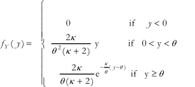
It is useful to redefine the second parameter, denoting κ=λ·θ. Therefore, we can write the p.d.f. in a simpler way:

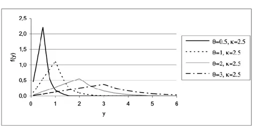
2 ( ) 0 if 0 2 ( ) y if 0 y ( 2 ) 2 _{e if y} ( 2 ) Y y y f y κ θ θ κ _θ θ κ κ _θ θ κ − − ⎧ ⎪ < ⎪ ⎪⎪ = _⎨ < < + ⎪ ⎪ ⎪ _≥ ⎪ + ⎩ (24)

where θ > 0, κ > 0. In Figure 1 we have represented the p.d.f. as a function of κ; in Figure 2, we have represented it as a function of θ.

Figure 11 – Two-faced probability density function (κ =2.5, θ ̣variable)

The cumulative distribution function FY(y) can be easily derived by integrating

the density function given in (24):

2 2 ( ) 0 if 0 ( ) y if 0 y ( 2) 2e 1 if y 2 Y y y F y κ _θ θ κ _θ θ κ θ κ − − ⎧ < ⎪ ⎪ ⎪ ⎪ =_⎨ < < + ⎪ ⎪ ⎪ − ≥ ⎪ + ⎩ (25)

The hinge point y = θ is the mode. The p.d.f. and c.d.f. of such point are, re-spectively: 2 2 ( ) , ( ) 2 ( 2) 2 Y Y f θ λ κ F θ κ λθ θ κ κ = = = + + + (26)

If κ is less, equal or greater than 2, the median is less, equal or greater than θ. The Expected value of a two-faced distribution is to be calculated by solving two integrals, corresponding, respectively, to values less and greater than θ. It is useful to start from the expression of p.d.f. given in (23).

Left Integral (from 0 to θ):

3 2 2 0 0 2 3 3( 2) L I y dy y dy θ θ _{αθ κθ} α α κ = = = = +

∫

∫

Right Integral (from θ to +∞): - -2 2 ( 1) 2 1 ye ye 2 ( 2) y y e RI dy dy e λθ λ λ λθ θ θ λθ λ λθ β β λθ λ λ λθ +∞ +∞ − + + = = = = + +

∫

∫

Applying the usual simplifying notation κ = λθ, we have: 2 ( 1) ( 2) RI θ κ κ κ + = + (29)

Adding these two components we derive the expected value E(Y):

2 2 2 ( 1) 2 6 ( 1) 2( 3 3) 2 ( ) 3( 2) ( 2) 3 ( 2) 3 ( 2) E Y LI RI κθ θ κ κ θ θ κ κ κ θ κ κ κ κ κ κ κ + + + + + = + = + = = + + + + (30)

In Table 5 we have specified the expected value of a two-faced variable Y for some parameter values:

TABLE 5

Expected value of TF distribution for some parameter values

κ = 0.5 1 1.5 2 6 3 5 10 θ = 0.5 1.267 0.778 0.619 0.542 0.500 0.467 0.410 0.369 1 2.533 1.556 1.238 1.083 1.000 0.933 0.819 0.739 2 5.067 3.111 2.476 2.167 2.000 1.867 1.638 1.478 3 7.600 4.667 3.714 3.250 3.000 2.800 2.457 2.217 4 10.133 6.222 4.952 4.333 4.000 3.733 3.276 2.956 6 15.200 9.333 7.429 6.500 6.000 5.600 4.914 4.433 8 20.267 12.444 9.905 8.667 8.000 7.467 6.552 5.911 10 25.333 15.556 12.381 10.833 10.000 9.333 8.190 7.389

In particular, when κ is equal to 6 , then we have E(Y) = θ. Indeed, if we put

κ= 6 in (30), we have: 2 (6 3 6 3) 2(9 3 6) ( ) . 3 6 ( 6 2) 18 6 6 E Y = θ + + = + θ θ= + + (31)

Coming back to the general TF distribution, and using an analogous method, we derive the second moment:

3 2 2 2 2 4 8 8 ( ) 2 ( 2) E Y κ κ κ θ κ κ + + + = + (32)

4 3 2 2 2 2 2 2 6 24 72 72 ( ) ( ) [ ( )] 18 ( 2) V Y E Y E Y κ κ κ κ θ κ κ + + + + = − = + . (33)

In Table 6 we have computed the variance of a two-faced variable Y for some parameter values:

TABLE 6

Variance of TF distribution for some parameter values

κ = 0.5 1 1.5 2 3 4 5 10 θ = 0.5 1.021 0.270 0.131 0.082 0.046 0.033 0.027 0.019 1 4.082 1.080 0.523 0.326 0.184 0.133 0.109 0.074 2 16.33 4.321 2.091 1.306 0.738 0.534 0.437 0.296 3 36.74 9.722 4.704 2.938 1.660 1.201 0.982 0.666 4 65.32 17.28 8.363 5.222 2.951 2.136 1.747 1.185 6 146.96 38.89 18.82 11.75 6.640 4.806 3.930 2.666 8 261.26 69.14 33.45 20.89 11.80 8.543 6.986 4.739 10 408.22 108.02 52.27 32.64 18.44 13.35 10.92 7.404

Following the same pattern, we can easily derive the third and fourth moment of a TF distribution: 4 3 2 3 3 3 2( 5 15 30 30 ) ( ) 5 ( 2) E Y κ κ κ κ θ κ κ + + + + = + (34) 5 4 3 2 4 4 4 6 24 72 144 144 ( ) 3 ( 2) E Y κ κ κ κ κ θ κ κ + + + + + = + (35)

and give a general formula for the m-th moment:

0 ! ( 2) ! 2 ( ) 2 2 m j m j m m m m j E Y m κ κ θ κ − = + + = + +

∑

of skewness (γ1) and kurtosis (γ2). It is worth to observe that indices γ1 and γ2 do

not depend on θ, due to the fact that moments are directly proportional to the corresponding powers of the parameter θ itself. We have reported, in Table 7, the first four moments, as well as the standard deviation S(Y), and the indices of skewness γ1 and kurtosis γ2.

Looking at Table 3, we realise that moments are inversely correlated with κ; the level of skewness depends only on κ, being γ1 positive for small values of this parameter and negative for larger values. The value of κ corresponding to γ1=0 is,

approximately, κ = 6.15. Νevertheless, ιn this context, the p.d.f. will not be per-fectly symmetric, having limited left tail and unlimited right tail, so this specific result seems to deserve some attention. Kurtosis, as well, decreases as κ becomes

larger, and the TF may be leptokurtic (small values of κ) or platikurtic (large val-ues of κ). The threshold value is approximately κ = 6.47, corresponding to a normokurtic distribution (with γ2=3, as in Gaussian model). It is interesting that

threshold values, respectively corresponding to γ1=0 andγ2=0, are not coinciding

but quite near to each other.

TABLE 7

Moments of TF distribution and related statistics

κ E (Y) E (Y2_{) E(Y}3_{) E(Y}4_{) S(Y) γ1 γ2}

0.5 2.533 θ 10.500 θ2 _{63.280 θ}3 _{506.467 θ}4 _{2.020 θ 1.939 8.760} 1 1.556 θ 3.500 θ2 _{10.800 θ}3 _{43.444 θ}4 _{1.039 θ 1.777 8.136} 2 1.083 θ 1.500 θ2 _{2.575 θ}3 _{5.417 θ}4 _{0.571 θ 1.302 6.465} √6 θ 1.242 θ2 _{1.853 θ}3 _{3.300 θ}4 _{0.492 θ 1.070 5.763} 3 0.933 θ 1.056 θ2 _{1.396 θ}3 _{2.141 θ}4 _{0.429 θ 0.834 5.032} 4 0.861 θ 0.875 θ2 1.006 θ3 1.295 θ4 0.365 θ 0.469 4.074 5 0.819 θ 0.780 θ2 _{0.825 θ}3 _{0.955 θ}4 _{0.330 θ 0.207 3.481} 6 0.792 θ 0.722 θ2 _{0.724 θ}3 _{0.782 θ}4 _{0.309 θ 0.023 3.119} 8 0.758 θ 0.656 θ2 _{0.616 θ}3 _{0.615 θ}4 _{0.285 θ -0.203 2.749} 10 0.739 θ 0.620 θ2 _{0.561 θ}3 _{0.536 θ}4 _{0.272 θ -0.324 2.590} 15 0.714 θ 0.576 θ2 _{0.497 θ}3 _{0.450 θ}4 _{0.257 θ -0.456 2.458}

7. PARAMETER ESTIMATION FOR A TWO – FACED DISTRIBUTION

The two-faced distributions, as defined and described above has two parame-ters to estimate: the hinge point θ and the shape parameter κ. If the hinge point value, say θ0, is known, say the ML estimator of the shape parameter is:

0 0 0 ˆ 1 2 -1 ( _j ) y j n y θ θ κ θ > = + −

∑

and it depends, essentially, on the right tail values of the sample. The main prob-lem is to estimate θ, when unknown, since the p.d.f. depends directly on its value. Being θ the modal point, the following step-by-step procedure seems suitable:

a) Find the sample subset where the points seem to be more dense, thus identi-fying a set of (say) n’ sample values which are not too far from each other;

b) Let θ be equal to each of the n’ points belonging to the subset and calculate the corresponding maximum likelihood estimate κ* by applying (35). We find, with this method, n’ couples of parameter estimates {θj*, κj*; j= 1,2,..., n’}

c) Calculate the log-likelihood of each couple of parameter estimates, and con-sider the couple (θ**, κ**), yielding the maximum log-likelihood;

d) Change slightly the value of θ** in both directions; if the resulting likelihood does not decrease, we can keep the couple (θ**, κ**) as a maximum likelihood estimation.

A specifical socio-demographic application of the TF distribution has been proposed in Brizzi (2006), concerning the distribution of municipal population of Emilia – Romagna, a region of northern Italy having a little more than 300 mu-nicipalities. The TF model resulted to be very well-fitting for such set of data.

7. CONCLUDING REMARKS

There are many natural and social phenomena having a different behaviour, depending on we are considering values which are smaller or greater than a threshold point. The distribution models representing variables related with such kind of phenomena do need to have a different shape on the left and on the right of the above mentioned threshold value, which becomes the hinge point of the distribution. It is surely useful to dispose of general models, which may include a great variety of particular cases; families of distributions like STSP, MTSP and TF, developed in this paper, may be appropriate in such context, due to the wide range of models included. Evidently, this subject is worth of further investigation, and it would be surely possible and useful to derive new hinge-point models by modifying or generalising the distribution families considered here. For instance, the triangular-exponential TF distribution may be extended by changing the shape of right tail section, which may allow us to define a triangular-gamma dis-tribution, a triangular-gaussian and so on. It is also possible to define models with more that one hinge point. As always, such “new” models should be fitted to real data, in order to check their capability to represent some specific natural or social variable. Even here, as in many other fields, theory can give useful tools to prac-tice, and practice may give a strong validation to theory.

Dipartimento di Scienze statistiche “Paolo Fortunati” MAURIZIO BRIZZI

Università di Bologna

ACKNOWLEDGEMENTS

The Author is deeply grateful to prof. Samuel Kotz (George Washington University) for discussing the main features of this paper and giving a lot of useful suggestions.

REFERENCES

M. BRIZZI (2006), A skewed model combining triangular and exponential features: the two – faced dis-tribution and its statistical properties, “Austrian Journal of Statistics”, 35, pp. 455-462. N.L. JOHNSON (1997), The triangular distribution as a proxy for the Beta distribution in risk analysis,

“The Statistician”, 46, pp. 387-398.

N.L. JOHNSON, S. KOTZ(1999),Non–smooth sailing or triangular distributions revisited after some 50 years, “The Statistician”, 48, pp. 179-187.

J.R. VAN DORP, S. KOTZ (2002a), The standard two-sided power distribution and its properties, with ap-plications to financial engineering, “The American Statistician”, 56, pp. 90-99.

J.R. VAN DORP, S. KOTZ (2002b), A novel extension of triangular distribution and its parameter estima-tion, “The Statistician”, 51, pp. 63-79.

J.R. VAN DORP, S. KOTZ (2003), Generalized trapezoidal distributions, “Metrika”, 58, pp. 85-97.

SUMMARY

Some considerations and developments about recently proposed families of distributions with hinge points This paper deals with probability density functions with hinge points, useful when rep-resenting phenomena which have different statistical features, depending on the fact that a threshold point has been overtaken or not. The STSP distribution, proposed by Van Dorp and Kotz (2002 a) is recalled and developed, and a modified model (MTSP), a mix-ture of STSP and Uniform, is defined and studied. Moreover, the Two Faced distribution, already proposed in Brizzi (2006), is recalled and thoroughly analysed, and some estima-tion problems, related to both models considered, are faced by a semi-empirical approach.