UNIVERSITY
OF TRENTO
DEPARTMENT OF INFORMATION AND COMMUNICATION TECHNOLOGY
38050 Povo – Trento (Italy), Via Sommarive 14
http://www.dit.unitn.it
REASONING WITH GOAL MODELS
Paolo Giorgini, Eleonora Nicchiarelli,
John Mylopoulous and Roberto Sebastiani
2002
Technical Report # DIT-02-0043
Also: In Proc. "Int. Conference of Conceptual Modeling -- ER2002"
Tampere, Finland, October 2002. LNCS series, © Springer Verlag.
Paolo Giorgini1, John Mylopoulos2, Eleonora Nicchiarelli1, and Roberto Sebastiani1
1 Department of Information and Communication Technology
University of Trento - Italy
{pgiorgini,eleonora,rseba}@science.unitn.it
2 Computer Science Department - University of Toronto - Canada
Abstract. Over the past decade, goal models have been used in Com-puter Science in order to represent software requirements, business objec-tives and design qualities. Such models extend traditional AI planning techniques for representing goals by allowing for partially defined and possibly inconsistent goals. This paper presents a formal framework for reasoning with such goal models. In particular, the paper proposes a qual-itative and a numerical axiomatization for goal modeling primitives and introduces label propagation algorithms that are shown to be sound and complete with respect to their respective axiomatizations. In addition, the paper reports on preliminary experimental results on the propagation algorithms applied to a goal model for a US car manufacturer.
1
Introduction
The concept of goal has been used in many areas of Computer Science for quite some time. In AI, goals have been used in planning to describe desirable states of the world since the 60s [5]. More recently, goals have been used in Software Engineering to model early requirements [2] and non-functional requirements [4] for a software system. For instance, an early requirement for a library information system might be “Every book request will eventually be fulfilled”, while “The new system will be highly reliable” is an example of a non-functional requirement. Goals are also useful for knowledge management systems which focus on strategic knowledge, e.g., “Increase profits”, or “Become the largest auto manufacturer in North America” [3].
Traditional goal analysis consists of decomposing goals into subgoals through an AND- or OR-decomposition. If goal G is AND-decomposed (respectively, OR-decomposed) into subgoals G1, G2, . . . , Gn, then if all (at least one) of the subgoals are satisfied so is goal G. Given a goal model consisting of goals and AND/OR relationships among them, and a set of initial labels for some nodes
?We would like to thank Greg McArthur for sharing with us a version of his goal
model for car manufacturing. We also thank the anonymous reviewers and Greg McArthur for helpful feedback on earlier drafts of this paper.
of the graph (S for Satisfied, D for Denied) there is a simple label propagation algorithm which can generate labels for all other nodes of the graph [6].
Unfortunately, this simple framework for modeling and analyzing goals won’t work for many domains where goals are not formalizable and the relationships among them can’t be captured by semantically well-defined relations such as AND/OR ones. For example, goals such as “Highly reliable system” have no for-mally defined predicate which prescribes their meaning, though one may want to define necessary conditions for such a goal to be satisfied. Moreover, such a goal may be related to other goals, such as “Thoroughly debugged system”, “Thoroughly tested system” in the sense that the latter obviously contribute to the satisfaction of the former, but this contribution is partial and qualitative. In other words, if the latter goals are satisfied, they certainly contribute to the satisfaction of the former goal, but don’t guarantee its satisfaction. The frame-work will also not frame-work in situations where there are contradictory contributions to a goal. For instance, we may want to allow for multiple decompositions of a goal G into sets of subgoals, where some decompositions suggest satisfaction of G while others suggest denial.
We are interested in a modeling framework for goals which allows for other, more qualitative goal relationships and can accommodate contradictory situa-tions. We accomplish this by introducing goal relationships labelled “+” and “–” which model respectively a situation where a goal contributes positively or negatively towards the satisfaction of another goal.
A major problem that arises from this extension is giving a precise semantics to the new goal relationships. This is accomplished in two different ways in this paper. In section 3 we offer a qualitative formalization and a label propagation algorithm which is shown to be sound and complete with respect to the formal-ization. In section 4, we offer a quantitative semantics for the new relationships which is based on a probabilistic model, and a label propagation algorithm that is also shown to be sound and complete. Section 5 presents preliminary experi-mental results on our label propagation algorithms, while section 6 summarizes the contributions of the paper and sketches directions for further research.
2
An Example
Suppose we are modeling the strategic objectives of a US car manufacturer, such as Ford or GM. Examples of such objectives are increase return on investment or increase customer loyalty. Objectives can be represented as goals, and can be analyzed using goal relationships such as AND, OR, “+” and “−”. In addition, we will use ”++” (respectively ”−−”) a binary goal relationship such that if ++(G,G’) (−−(G,G’)) then satisfaction of G implies satisfaction (denial) of G’. For instance, increase return on investment may be AND-decomposed into increase sales volume and increase profit per vehicle. Likewise, increase sales volume might be OR-decomposed into increase consumer appeal and expand markets. This decomposition and refinement of goals can continue until we have goals that are tangible (i.e., someone can satisfy them through an appropriate course
increase profit per vehicle price lower gas mileage improve appeal consumer increase increase sales price keep labour costs low price rises
US gas Japanese gasprice rises
Yen rises rates rise Japanese lower Jap. interest rates sales increase volume increase Toyota sales markets expand earningsforeign increase production costs lower sales high margin increase improve production economies of materials costs
reduce raw outsource productionunits of + rebates offer price lower sales loan interst rates lower costs purchaselower environment impact lower costs operating reduce price rises gas + + + + + + + increase customer loyalty qualitycar improve servicescar improve + + + increase return on investment (GM) increase sales VW −S −S −S OR AND OR AND OR OR OR −− OR − − − − −
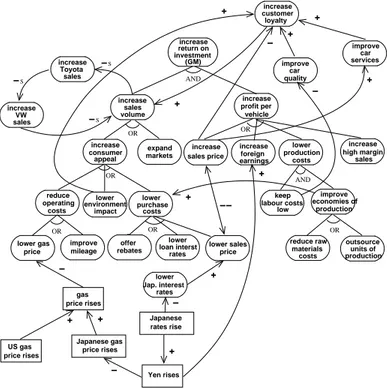
Fig. 1.A partial goal model for GM.
of action) and/or observable (i.e., they can be confirmed satisfied/denied by simply observing the application domain).
For vaguely stated goals, such as increase customer loyalty we may want to simply model other relevant goals, such as improve car quality, improve car services and relate them through “+” and “−” relationships, as shown in Figure 1. These goals may influence positively or negatively some of the goals that have already been introduced during the analysis of the goal increase return on investment. Such lateral goal relationships may introduce cycles in our goal models.
Examples of observable goals are Yen rises, gas prices rise etc. When such a goal is satisfied, we will call it an event (the kind of event you may read about in a news story) and represent it in our graphical notation as a rectangle (see lower portion of Figure 1).
Figure 1 shows a partial and fictitious goal model for GM focusing on the goal increase return of investment. In order to increase return of investment, GM has to satisfy both goals increase sales and increase profit per vehicle. In turn, increase sales volume is OR-decomposed into increase consumer appeal and expand markets, while the goal increase profit per vehicle is OR-decomposed into increase sales price, lower production costs, increase foreign earnings, and increase high margin sales. Additional decompositions are shown in the figure. For instance, the goal increase consumer appeal can be satisfied by satisfying lower environment impact, trying to lower purchase costs, or reducing the vehicle operating costs (reduce operating costs).
The graph shows also lateral relationships among goals. For example, the goal increase customer loyalty has positive (+) contributions from goals lower environment impact, improve car quality and improve car services, while it has a negative (−) contribution from increase sales price. The root goal increase return on investment (GM) is also related with goals concerning others auto manufac-turer, such as Toyota and VW. In particular, if GM increases sales, then Toyota loses a share of the North American market; if Toyota increases sales increase Toyota sales), it does so at the expense of VW; finally, if VW increases sales (increase VW sales), it does so at the expense of GM.
So far, we have assumed that every goal relationship treats S and D in a dual fashion. For instance, if we have +(G,G’), then if G is satisfied, G’ is partially satisfied, and (dually) if G is denied G’ is partially denied. Note however, that sometimes a goal relationship only applies for S (or D). In particular, the – contribution from increase sales (GM) to increase sales (Toyota) only applies when increase sales (GM) is satisfied (if GM hasn’t increased sales, this doesn’t mean that Toyota has.) To capture this kind of relationship, we introduce −S, −D, +S, +D (see also Figure 1). Details about the semantics of these are given in the next section.
3
Qualitative Reasoning with Goal Models
Formally, a goal graph is a pair hG, Ri where G is a set of goals and R is a set of goal relations over G. If (G1, ..., Gn) 7−→ G is a goal relation in R, we callr G1...Gn source goals and G the target goal of r. To simplify the discussion, we consider only binary OR and AN D goal relations. This is not restrictive, as all the operators we consider in this section and in Section 4 —i.e., ∧, ∨, min, max, ⊗, ⊕— are associative and can be thus trivially used as n-ary operators. 3.1 Axiomatization of goal relationships
Let G1, G2, ...denote goal labels. We introduce four distinct predicates over goals, F S(G), F D(G) and P S(G), P D(G), meaning respectively that there is (at least) full evidence that goal G is satisfied and that G is denied, and that there is at least partial evidence that G is satisfied and that G is denied. We also use the proposition > to represent the (trivially true) statement that there is at least null evidence that the goal G is satisfied (or denied). Notice that the predicates state that there is at least a given level of evidence, because in a goal graph there may be multiple sources of evidence for the satisfaction/denial of a goal. We introduce a total order F S(G) ≥ P S(G) ≥ > and F D(G) ≥ P D(G) ≥ >, with the intended meaning that x ≥ y iff x → y.
We want to allow the deduction of positive ground assertions of type F S(G), F D(G), P S(G) and P D(G) over the goal constants of a goal graph. We refer to externally provided assertions as initial conditions. To formalize the propa-gation of satisfiability and deniability evidence through a goal graph hG, Ri, we introduce the axioms described in Figure 2. (By “dual” we mean that we invert satisfiability with deniability.)
Goal Invariant Axioms
G: F S(G) → P S(G) (1) F D(G) → P D(G) (2) Goal relation Relation Axioms
(G2, G3) and 7−→G1: (F S(G2) ∧ F S(G3)) → F S(G1) (3) (P S(G2) ∧ P S(G3)) → P S(G1) (4) F D(G2) → F D(G1), F D(G3) → F D(G1) (5) P D(G2) → P D(G1), P D(G3) → P D(G1) (6) G27−→+S G1: P S(G2) → P S(G1) (7) G2 −S 7−→G1: P S(G2) → P D(G1) (8) G2 ++S 7−→ G1: F S(G2) → F S(G1), (9) P S(G2) → P S(G1) (10) G2 −−S 7−→ G1: F S(G2) → F D(G1), (11) P S(G2) → P D(G1) (12)
Fig. 2.Ground axioms for the invariants and the propagation rules in the qualitative reasoning framework. The (or), (+D), (−D), (++D), (−−D) cases are dual w.r.t. (and),
(+S), (−S), (++S), (−−S) respectively.
As indicated in Section 2, the propagation of goal satisfaction through a ++, −−, +, − may or may not be symmetric w.r.t. that of denial. Thus, for every relation type r ∈ {++, −−, +, −}, it makes sense to have three possible labels: ”rS”, ”rS”, and ”r”, meaning respectively that satisfaction is propagated, that denial is propagated, and that both satisfaction and denial are propagated. (We call the first two cases asymmetric, the latter symmetric.) For example, G2
−S
7−→ G1 means that if G2 is satisfied, then there is some evidence that G1is denied, but if G2is denied, then nothing is said about the satisfaction of G1; G2
−D
7−→ G1 means that if G2 is denied, then there is some evidence that G1is satisfied, but if G2 is satisfied, then nothing is said about the denial of G1; G2
−
7−→ G1means that, if G2 is satisfied [denied], then there is some evidence that G1 is denied [satisfied]. In other words, a symmetric relation G2 7−→ Gr 1 is a shorthand for the combination of the two corresponding asymmetric relationships G2
rS
7−→ G1 and G2
rD
7−→ G1.
(1) and (2) state that full satisfiability and deniability imply partial satisfi-ability and denisatisfi-ability respectively. For an AND relation, (3) and (4) show that the full and partial satisfiability of the target node require respectively the full and partial satisfiability of all the source nodes; for a “+S” relation, (7) show that only the partial satisfiability (but not the full satisfiability) propagates through a “+S” relation. Combining (1) with (3), and (1) with (7), we have, respectively,
(G2, G3) and 7−→ G1: (F S(G2) ∧ P S(G3)) → P S(G1) (13) G2 +S 7−→ G1: F S(G2) → P S(G1). (14)
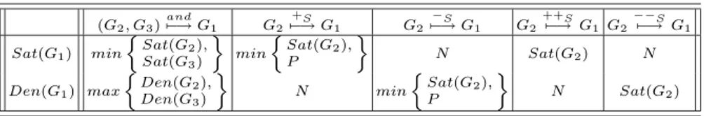
Thus, an AND relation propagates the minimum satisfiability value (and the maximum deniability one), while a “+S” relation propagates at most a partial satisfiability value.
(G2, G3) and 7−→G1 G2 +S 7−→G1 G27−→−S G1 G2 ++S 7−→ G1 G2−−S7−→ G1 Sat(G1) min nSat(G 2), Sat(G3) o min nSat(G 2), P o N Sat(G2) N Den(G1) max nDen(G 2), Den(G3) o N min nSat(G 2), P o N Sat(G2)
Table 1. Propagation rules in the qualitative framework. The (or), (+D), (−D),
(++D), (−−D) cases are dual w.r.t. (and), (+S), (−S), (++S), (−−S) respectively.
From now on, we implicitly assume that axioms (1) and (2) are always ap-plied whenever possible. Thus, we say that P S(G1) is deduced from F S(G2) and F S(G3) by applying (3) —meaning “applying (3) and then (1)”— or that P S(G1) is deduced from F S(G2) and P S(G3) by applying (4) —meaning “ap-plying (1) and then (4)”.
We say that an atomic proposition of the form F S(G), F D(G), P S(G) and P D(G) holds if either it is an initial condition or it can be deduced via modus ponens from the initial conditions and the ground axioms of Figure 2. We assume conventionally that > always holds. Notice that all the formulas in our framework are propositional Horn clauses, so that deciding if a ground assertion holds not only is decidable, but also it can be decided in polynomial time.
We say that there is a weak conflict if either P S(G) and P D(G), F S(G) and P D(G), P S(G) and F D(G) hold for some goal G. We say that there is a strong conflict if F S(G) and F D(G) hold for some G.
3.2 The label propagation algorithm
Based on the logic framework of Section 3.1, we have developed an algorithm for propagating through a goal graph hG, Ri labels representing evidence for the satisfiability and deniability of goals. To each node G ∈ G we associate two variables Sat(G), Den(G) ranging in {F, P, N } (full, partial, none) such that F > P > N, representing the current evidence of satisfiability and deniability of goal G. For example, Sat(Gi) ≥ P states that there is at least partial evidence that Giis satisfiable. Starting from assigning an initial set of input values for Sat(Gi), Den(Gi) to (a subset of) the goals in G, we propagate the values through the goal relations in R according to the propagation rules of Table 1.
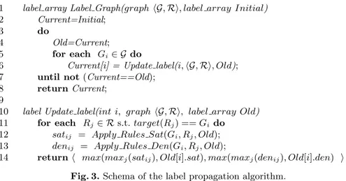
The schema of the algorithm is described in Figure 3. Initial, Current and Oldare arrays of |G| pairs hSat(Gi), Den(Gi)i, one for each Gi∈ G, representing respectively the initial, current and previous labeling states of the graph. We call the pair hSat(Gi), Den(Gi)i a label for Gi. Notationally, if W is an array of labels hSat(Gi), Den(Gi)i, by W [i].sat and W [i].den we denote the first and second field of the ith label of W .
The array Current is first initialized to the initial values Initial given as input by the user. At each step, for every goal Gi, hSat(Gi), Den(Gi)i is updated by propagating the values of the previous step. This is done until a fixpoint is reached, in the sense that no further updating is possible (Current == Old).
The updating of hSat(Gi), Den(Gi)i works as follows. For each relation Rj incoming in Gi, the satisfiability and deniability values satij and denij derived
1 label array Label Graph(graph hG, Ri, label array Initial)
2 Current=Initial;
3 do
4 Old=Current;
5 for each Gi∈ G do
6 Current[i] = Update label(i, hG, Ri, Old);
7 until not(Current==Old);
8 returnCurrent;
9
10 label Update label(int i, graph hG, Ri, label array Old) 11 for each Rj∈ R s.t. target(Rj) == Gido
12 satij = Apply Rules Sat(Gi, Rj, Old);
13 denij = Apply Rules Den(Gi, Rj, Old);
14 returnh max(maxj(satij), Old[i].sat), max(maxj(denij), Old[i].den) i
Fig. 3.Schema of the label propagation algorithm.
from the old values of the source goals are computed by applying the rules of Table 1. The result is compared with the old value, and the maximum is returned as new value for Gi.
3.3 Termination and complexity
Theorem 1. Label Graph(hG, Ri, Initial) terminates after at most 6|G|+1 loops. Proof. First, from lines 6 and 14 in Figure 3 we have that, for every goal Gi,
Current[i].sat = max(..., Old[i].sat), Current[i].den = max(..., Old[i].den)
so that their values are monotonically non-decreasing. In order not to terminate, at least one value per step should monotonically increase. Each of the 2|G| vari-ables Sat(Gi) and Den(Gi) admits 3 possible values and at each non-final loop at least one value increases. Thus the procedure must terminate after at most
6|G| + 1 loops. 2
Notice that the upper bound is very pessimistic, as many value updates are done in parallel. In Section 5, we report on experiments we have conducted which suggest that the algorithm generally converges after a few loops.
3.4 Soundness and completeness
We call a value statement an expression of the form (v ≥ c), v ∈ {Sat(Gi), Den(Gi)} for some goal Giand c ∈ {F, P, N }, with the intuitive meaning “there is at least evidence c for v”. Thus from now on we rewrite the assertion F S(G), P S(G), > as (Sat(G) ≥ F ), (Sat(G) ≥ P ), (Sat(G) ≥ N ) and F D(G), P D(G), > as (Den(G) ≥ F ), (Den(G) ≥ P ), (Sat(G) ≥ N ) respectively.
We say that (v1≥ c1) is deduced from (v2≥ c2) [and (v3≥ c3)] by a relation axiom meaning that the corresponding assertions are deduced. For instance, (Sat(G1) ≥ P ) is deduced from (Sat(G2) ≥ F ) by axiom (7) as P S(G1) is deduced from F S(G2) by axiom (7).
We say that (v1≥ c1) derives from (v2≥ c2) [and (v3≥ c3)] by means of one propagation rule x = f (y, z) [x = f (y)] of Table 1 if c1= f (c2, c3) [c1= f (c2)]. For instance, (Sat(G1) ≥ P ) derives from (Sat(G2) ≥ P ) and (Sat(G3) ≥ F ) by means of the first propagation rule. Notice that this is possible because the operators min and max are monotonic, that is, e.g., max(v1, v2) ≥ max(v01, v20) iff v1≥ v10 and v2≥ v20.
To this extent, the rules in Table 1 are a straightforward translation of the axioms (1)-(12), as stated by the following result.
Lemma 1. (v1 ≥ c1) derives from (v2 ≥ c2) [and (v3 ≥ c3)] by means of the propagation rules of Table 1 if and only if (v1 ≥ c1) is deduced from (v2 ≥ c2) [and (v3≥ c3)] with the application of one of the relation axioms (3)-(12). Proof. For short, we consider only the AND and +S cases for Sat(G1), as the other cases are either analogous or trivial and can be verified by the reader. (G2, G3)7−→ Gand 1: If either (Sat(G2) ≥ N ) or (Sat(G3) ≥ N ), then (Sat(G1) ≥ N )
is derived. This matches one-to-one the fact that from > nothing else is de-duced;
otherwise, if either (Sat(G2) ≥ P ) or (Sat(G3) ≥ P ), then (Sat(G1) ≥ P ) is derived. This matches one-to-one the fact that from (Sat(G2) ≥ P ) and (Sat(G3) ≥ P ) axiom (4) is applied, so that (Sat(G1) ≥ P ) is deduced; finally, if both (Sat(G2) ≥ F ) and (Sat(G3) ≥ F ), then (Sat(G1) ≥ F ). This matches one-to-one the fact that from (Sat(G2) ≥ F ) and (Sat(G3) ≥ F ), axiom (3) is applied, so that (Sat(G1) ≥ F ) is deduced.
G2 +S
7−→ G1: If (Sat(G2) ≥ N ), then (Sat(G1) ≥ N ). Again, this matches one-to-one the fact that from > nothing else is deduced;
otherwise, if either (Sat(G2) ≥ P ) or (Sat(G2) ≥ F ), then we have that Sat(G1) ≥ min(Sat(G2), P ) ≥ P . This matches one-to-one the fact that from either (Sat(G2) ≥ P ) or (Sat(G2) ≥ F ) axiom (7) is applied and
(Sat(G1) ≥ P ) is deduced. 2
Given an array of labels W , we say that (Sat(Gi) ≥ c) [resp. (Den(Gi) ≥ c)] is true in W if and only if W [i].sat ≥ c [resp. W [i].den ≥ c]. This allows us to state the correctness and completeness theorem for Label Graph().
Theorem 2. Let F inal be the array returned by Label Graph(hG, Ri, Initial). (v ≥ c) is true in F inal if and only if (v ≥ c) can be deduced from Initial by applying the relation axioms (3)-(12).
Proof. First we define inductively the notion of “deduced from Initial in k steps”: (i) an assertion in Initial can be deduced from Initial in 0 steps; (ii) an assertion can be deduced from Initial in up to k + 1 steps if either it can
be deduced from Initial in up to k steps or it can be deduced by applying a relation axiom to some assertions, all of which can be deduced from Initial in up to k steps.
Let Currentk be the value of Current after k loops. We show that (v ≥ c) is true in Currentk if and only if (v ≥ c) can be deduced from Initial in up to ksteps. The thesis follows from the fact that F inal = Currentk for some k.
We reason by induction on k. The base case k = 0 is obvious as Current0= Initial. By inductive hypothesis, we assume the thesis for k and we prove it for k+ 1.
If. Consider (v ≥ c) such that (v ≥ c) is deduced from Initial in up to k + 1 steps. Thus, (v ≥ c) is obtained by applying some relation axiom AX to some assertion(s) (v1≥ c1) [and (v2≥ c2)], which can be both deduced from Initialin up to k steps. Thus, by inductive hypothesis, (v1≥ c1) [and (v2≥ c2)] occur in Currentk. Then, by Lemma 1, (v ≥ c) derives from (v1 ≥ c1) [and (v2 ≥ c2)] by means of the propagation rules of Table 1. Thus, if v is Sat(Gi) [resp Den(Gi)], then c is one of the values satij [resp. denij] of lines 14, 15 in Figure 3, so that Currentk+1[i].sat ≥ c [Currentk+1[i].den ≥ c]. Thus (v ≥ c) is true in Currentk+1.
Only if. Consider a statement (v ≥ c) true in Currentk+1. If (v ≥ c) is true also in Currentk, then by inductive hypothesis (v ≥ c) can be deduced from Initialin up to k steps, and hence in k+1 steps. Otherwise, let Rjbe the rule and let (v2 ≥ c2) [and (v3 ≥ c3)] the statements(s) true in Currentk from which v has been derived. By inductive hypothesis (v2≥ c2) [and (v3≥ c3)] can be deduced from Initial in up to k steps. By Lemma 1 (v ≥ c) can be deduced from (v2 ≥ c2) [and (v3 ≥ c3)] by the application of one relation axiom, and thus can be deduced from Initial in up to k + 1 steps. 2 Thus, from Theorem 2, the values returned by Label Graph(hG, Ri, Initial) are the maximum evidence values which can be deduced from Initial.
4
Quantitative Reasoning with Goal Models
The qualitative approach of Section 3 allows for setting and propagating partial evidence about the satisfiability and deniability of goals and the discovery of conflicts.
We may want to provide a more fine-grained evaluation of such partial ev-idence. For instance, when we have G2 7−→ G+S 1, from P S(G2) we can deduce P S(G1), whilst one may argue that the satisfiability of G1 is in some way less evident than that of G2. For example, in the goal graph of Figure 1, the satisfac-tion of the goal Lower environment impact may not necessarily imply satisfacsatisfac-tion of Increase customer loyalty, so it may be reasonable to assume ”less evidence” for the satisfaction of the latter compared to the former. Moreover, the different relations which mean partial support – i.e., +S, −S, +D, −D – may have differ-ent strengths. For instance, in the goal graph of Figure 1, US Gas price rises
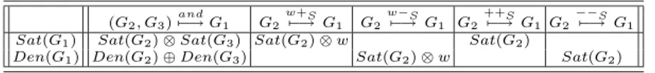
(G2, G3) and 7−→G1 G2 w+S 7−→ G1 G2 w−S 7−→ G1 G2 ++S 7−→ G1 G2−−S7−→G1
Sat(G1) Sat(G2) ⊗ Sat(G3) Sat(G2) ⊗ w Sat(G2)
Den(G1) Den(G2) ⊕ Den(G3) Sat(G2) ⊗ w Sat(G2)
Table 2. Propagation rules in the quantitative framework. The (or), (+D), (−D),
(++D), (−−D) cases are dual w.r.t. (and), (+S), (−S), (++S), (−−S) respectively.
may have a bigger impact on Gas price rises than Japanese gas price rises if the manufacturer’s market is mainly in the US.
To cope with these facts, we need a way for representing different numerical values of partial evidence for satisfiability/deniability and for attributing differ-ent weights to the +S, −S, +D, −D relations. And, of course, we also need a formal framework to reason with such quantitative information.
4.1 An extended framework
In our second attempt, we introduce a quantitative framework, inspired by [1]. We introduce two real constants inf and sup such that 0 ≤ inf < sup. For each node G ∈ G we introduce two real variables Sat(G), Den(G) ranging in the interval D =def[inf, sup], representing the current evidence of satisfiability and deniability of the goal G. The intended meaning is that inf represents no evidence, sup represents full evidence, and different values in ]inf, sup[ represent different levels of partial evidence.
To handle the goal relations we introduce two operators ⊗, ⊕ : D × D 7−→ D representing respectively the evidence of satisfiability of the conjunction and that of the disjunction [deniability of the disjunction and that of the conjunction] of two goals. ⊗ and ⊕ are associative, commutative and monotonic, and such that x⊗ y ≤ x, y ≤ x ⊕ y; there is also an implicit unary operator inv(), representing negation, such that inf = inv(sup), sup = inv(inf ), inv(x⊕y) = inv(x)⊗inv(y) and inv(x ⊗ y) = inv(x) ⊕ inv(y).
We also attribute to each goal relation +S, −S, +D, −D a weight w ∈ ]inf, sup[ stating the strength by which the satisfiability/deniability of the source goal influences the satisfiability/deniability of the target goal. The propagation rules are described in Table 2. As in the qualitative approach, a symmetric relation —such as, G2
w+
7−→ G1— is a shorthand for the combination of the two corresponding asymmetric relationships sharing the same weight w —e.g., G2
w+S
7−→ G1 and G2 w+D
7−→ G1.
There are a few possible models following the schema described above. In particular, here we adopt a probabilistic model, where the evidence of satisfiabil-ity Sat(G) [resp. deniabilsatisfiabil-ity Den(G)] of G is represented as the probabilsatisfiabil-ity that Gis satisfied (respectively denied). As usual, we adopt the simplifying hypothe-sis that the different sources of evidence are independent. Thus, we fix inf = 0, sup= 1, and we define ⊗, ⊕, inv() as:
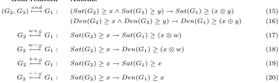
Goal relation Axioms (G2, G3)
and
7−→G1: (Sat(G2) ≥ x ∧ Sat(G3) ≥ y) → Sat(G1) ≥ (x ⊗ y) (15)
(Den(G2) ≥ x ∧ Den(G3) ≥ y) → Den(G1) ≥ (x ⊕ y) (16)
G2 w+S 7−→G1: Sat(G2) ≥ x → Sat(G1) ≥ (x ⊗ w) (17) G2w−S7−→G1: Sat(G2) ≥ x → Den(G1) ≥ (x ⊗ w) (18) G2 ++S 7−→G1: Sat(G2) ≥ x → Sat(G1) ≥ x (19) G2−−S7−→ G1: Sat(G2) ≥ x → Den(G1) ≥ x (20)
Fig. 4. Axioms for the propagation rules in the quantitative reasoning framework. The x, y variables are implicitly quantified universally. The (or), (+D), (−D), (++D),
(−−D) cases are dual w.r.t. (and), (+S), (−S), (++S), (−−S) respectively.
that is, respectively the probability of the conjunction and disjunction of two independent events of probability p1and p2, and that of the negation of the first event. To this extent, the propagation rules in Table 2 are those of a Bayesian network, where, e.g., in G2
w+S
7−→ G1 w has to be interpreted as the conditional probability P [G1 is satisf ied | G2 is satisf ied]. Notice that the qualitative framework of Section 3 can be seen as another such model with D = {F, P, N }, ⊗ = min() and ⊕ = max().3
4.2 Axiomatization
As with the qualitative case, we call a value statement an expression of the form (v ≥ c), v ∈ {Sat(Gi), Den(Gi)} for some Gi and c ∈ [0, 1], with the intuitive meaning “there is at least evidence c of v”. We want to allow the user to state and deduce non-negated value statements of the kind (Sat(G) ≥ c) and (Den(G) ≥ c) over the goal constants of the graph. We call externally provided assertions about the satisfaction/denial of goals initial conditions.
To formalize the propagation of satisfiability and deniability evidence values through a goal graph, for every goal and goal relation in hG, Ri, we introduce the axioms (15)-(20) in Figure 4. Unlike those of Figure 2, the relation axioms in Figure 4 are not ground Horn clauses —thus, propositional—but rather first-order closed Horn formulas, so that they require a first-first-order deduction engine. We say that a statement (v ≥ c) holds if either it is an initial condition or it can be deduced from the initial conditions and the axioms of Figure 4. We implic-itly assume that (Sat(Gi) ≥ 0) and (Den(Gi) ≥ 0) hold for every Gi, and that the deduction engine —either human or machine— can semantically evaluate ⊗ and ⊕ and perform deductions deriving from the values of the evaluated terms and the semantics of ≥. For instance, we assume that, if (G2, G3)
and
7−→ G1 is in R, then (Sat(G1) ≥ 0.1) can be deduced from (Sat(G2) ≥ 0.5), (Sat(G3) ≥ 0.4), as from (15) it is deduced (Sat(G1) ≥ 0.5 ⊗ 0.4), which is evaluated into (Sat(G1) ≥ 0.2), from which it can be deduced (Sat(G1) ≥ 0.1).
3 Another model of interest is that based on a serial/parallel resistance model, in
which inf = 0, sup = +∞, x ⊕ y = x + y, x ⊗ y = x·y
x+y and inv(x) = 1 x [1].
We say that there is a weak conflict if both (Sat(G) ≥ c1) and (Den(G) ≥ c2) hold for some goal G and constants c1, c2 > 0. We say that there is a strong conflict if there is a weak conflict s.t. c1= c2= 1.
4.3 The label propagation algorithm
Starting from the new numeric framework, we have adapted the label propaga-tion algorithm of Figure 3 to work with numeric values. The new version of the algorithm differs from that of Section 3 in that: the elements in Initial, Current and Old range in [0, 1]; the input graph contain also weights to the +S, −S, +D, −D goal relations; and, the propagation rules applied are those of Table 2. 4.4 Soundness and completeness
We say that (v1 ≥ c1) derives from (v2 ≥ c2) [and (v3 ≥ c3)] by means of one propagation rule x = f (y, z) [x = f (y)] of Table 2 if c1= f (c2, c3) [c1= f (c2)]. For instance, (Sat(G1) ≥ 0.4) derives from (Sat(G2) ≥ 0.8) and (Sat(G3) ≥ 0.5) by means of the first and propagation rule. Again, this is possible because the the operators ⊗ and ⊕ are monotonic.
Lemma 2. (v1 ≥ c1) derives from (v2 ≥ c2) [and (v3 ≥ c3)] by means of the propagation rules of Table 1 if and only if (v1 ≥ c1) is deduced from (v2 ≥ c2) [and (v3≥ c3)] with the application of one of the relation axioms (15)-(20). Proof. Trivial observation that the axioms (15)-(20) are straightforward trans-lation of the propagation rules in Table 1. 2 Given an array of labels W , we say that (Sat(Gi) ≥ c) [resp. (Den(Gi) ≥ c)] is true in W if and only if W [i].sat ≥ c [resp. W [i].den ≥ c]. This allows for stating the correctness and completeness theorem for Label Graph().
Theorem 3. Let F inal be the array returned by Label Graph(hG, Ri, Initial). (v ≥ c) is true in F inal if and only if (v ≥ c) can be deduced from Initial by applying the relation axioms (15)-(20).
Proof. Identical to that of Theorem 2, substituting the axioms (15)-(20) for the axioms (3)-(12), the rules in Table 2 for those in Table 1 and Lemma 2 for
Lemma 1. 2
Again, from Theorem 3, the values returned by Label Graph(hG, Ri, Initial) are the maximum evidence values which can be deduced from Initial.
4.5 Termination
To guarantee termination, the condition (Current == Old) of line 7 in Figure 3 is implemented as:
maxi(|Current[i].sat − Old[i].sat|) < ² and
maxi(|Current[i].den − Old[i].den|) < ²,
(21)
² being a sufficiently small real constant. (This is a standard practice to avoid numeric errors when doing computations with real numbers.) Thus, the algo-rithm loops until all satisfiability or deniability value variations have become negligible.
Theorem 4. Label Graph(hG, Ri, Initial) terminates in a finite number of loops. Proof. For the same reason as in Theorem 1, the values Current[i]k.sat and Current[i]k.den are monotonically non-decreasing with k. As every monotoni-cally non-decreasing upper-bounded sequence is convergent, both Current[i]k.sat and Current[i]k.denare convergent. Thus they are also Cauchy-convergent.4It follows that condition (21) becomes true after a certain number of loops. 2 Remark 1. In the proof of Theorem 3, we have assumed the terminating con-dition (Current == Old), whilst in our implementation we use concon-dition (21). Thus, whilst Label Graph() stops when (21) is verified, the corresponding deduc-tive process might go on, and thus deduce a value slightly bigger than the one returned by the algorithm. Since we can reduce ² at will, this “incompleteness” has no practical consequences.
5
Experimental Results
Both qualitative and quantitative algorithms have been implemented in Java and a series of tests were conducted on a Dell Inspiron 8100 laptop with a Pentium III CPU and 64 MB RAM (OS: GNU/Linux, kernel 2.4.7-10). The tests were intended to demonstrate the label propagation algorithms, also to collect some experimental results on how fast the algorithms converge.
The first set of experiments was carried out in order to demonstrate the qualitative label propagation algorithm. For each experiment, we assigned a set of labels to some of the goals and events of the auto manufacturer graph (Figure 1) and see their consequences for other nodes. The label propagation algorithm reached a steady state after at most five iterations.
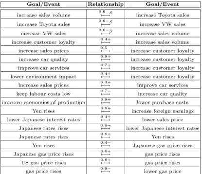
In a second set of experiments we assigned numerical weights to “+”, “−” and “−S” lateral relationships as reported in Table 3. For instance, the goal increase sales volume contributes negatively to the goal increase Toyota sales with a weight 0.6, while the goal increase car quality contributes positively to the goal increase customer loyalty with weight 0.8. Table 4 reports the results of four different experiments. For each goal/event, the table shows the initial (Init) label assignment to the variables S and D, also their final (Fin) value after label propagation. For instance, in the first experiment, the initial assignment for the goal expand markets is S=.3 and D=0, while the final values for increase return on investment (GM) are S=0 and D=.4.
The results of these experiments confirm those obtained with the qualitative algorithm. However, the numeric approach allows us to draw more precise con-clusions about the final value of goals. This is particularly helpful for evaluating contradictions. For instance, in the second experiment (Exp 2), even though we
4 An infinite sequence a
n is Cauchy-convergent if and only if, for every ² > 0, there
exist an integer N s.t. |an+1− an| < ² for every n ≥ N . anis convergent if and only
Goal/Event Relationship Goal/Event increase sales volume 0.6−S7−→ increase Toyota sales increase Toyota sales 0.6−S7−→ increase VW sales
increase VW sales 0.6−S7−→ increase sales volume increase customer loyalty 0.4+7−→ increase sales volume increase sales prices 0.5−7−→ increase customer loyalty increase car quality 0.8+7−→ increase customer loyalty improve car services 0.7+7−→ increase customer loyalty lower environment impact 0.4+7−→ increase customer loyalty
increase sales prices 0.3+7−→ improve car services keep labour costs low 0.7−7−→ increase car quality improve economies of production 0.8+7−→ lower purchase costs
Yen rises 0.8+7−→ increase foreign earnings lower Japanese interest rates 0.4+7−→ lower sales price
Japanese rates rises 0.8−7−→ lower Japanese interest rates Japanese rates rises 0.6+7−→ Yen rises
Yen rises 0.4−7−→ Japanese gas price rises Japanese gas price rises 0.6+7−→ gas price rises
US gas price rises 0.6+7−→ gas price rises gas price rises 0.8−7−→ lower gas price
Table 3.Quantitative relationships for the auto manufacturer example of Figure 2
have a contradiction for the final values of the root goal increase return on invest-ment (GM) (i.e., S=0.8 and D=0.4), we have more evidence for its satisfaction than its denial. With the qualitative approach we had S=P and D=P, and there was nothing else to say about this contradiction. Analogous comments apply for the fourth experiment.
The threshold ² (equation 21) used in the experiments has been chosen as the smallest positive value of type float (i.e., Float.MIN VALUE). With this threshold, the algorithm converged in five iterations for all four experiments.
6
Conclusions
We have presented a formal framework for reasoning with goal models. Our goal models use AND/OR goal relationships, but also allow more qualitative relationships, as well as contradictory situations. A precise semantics has been given for all goal relationships which comes in a qualitative and a numerical form. Moreover, we have presented label propagation algorithms for both the qualitative and the numerical case that are shown to be sound and complete with respect to their respective axiomatization. Finally, the paper reports some preliminary experimental results on the label propagation algorithms applied to a goal model for a US car manufacturer.
Future research directions include applying different techniques, such as Demp-ster Shafer theory [7], to take into consideration the sources of information in the propagation algorithms. This will allow us to consider, for instance, the reli-ability and/or the competence of a source of evidence . We also propose to apply our framework to more complex real cases to confirm its validity.
Exp 1 Exp 2 Exp 3 Exp 4 Goals/Events Init Fin Init Fin Init Fin Init Fin
S D S D S D S D S D S D S D S D increase return on investment (GM) 0 0 0 .4 0 0 .8 .4 0 0 .9 .2 0 0 .9 .6 increase sales volume 0 0 1 .1 0 0 1 .1 0 0 1 .2 0 0 1 .6 increase profit per vehicle 0 0 0 .4 0 0 .8 .4 0 0 .9 0 0 0 .9 0 increase customer appeal 0 0 1 0 0 0 1 0 0 0 1 0 0 0 1 0 expand markets .3 0 .3 0 .3 0 .3 0 .3 0 .3 0 .3 0 .3 0 increase sales price 0 .5 0 .8 0 .5 0 .8 0 .5 0 .8 0 .5 0 .8 increase foreign earnings 0 .9 0 .9 0 .9 .8 .9 0 .9 .8 .9 0 .9 .8 .9 lower production costs 0 0 0 .9 0 0 0 .9 0 0 .6 0 0 0 .6 0 increase high margin sales 0 .6 0 .6 0 .6 0 .6 0 .6 0 .6 0 .6 0 .6 reduce operating costs 0 0 .8 0 0 0 .8 0 0 0 .8 0 0 0 .8 0 lower environmental impact .9 0 .9 0 .9 0 .9 0 .9 0 .9 0 .9 0 .9 0 lower purchase costs 0 0 .9 0 0 0 .9 0 0 0 .9 0 0 0 .9 0 keep labour costs low 0 .9 0 .9 0 .9 0 .9 .9 0 .9 0 .9 0 .9 0 improve economies of production 0 0 0 0 0 0 0 0 0 0 .7 0 0 0 .7 0 improve mileage 0 0 0 0 0 0 0 0 0 0 0 0 0 0 0 0 lower gas price .8 0 .8 0 .8 0 .8 0 .8 0 .8 0 .8 0 .8 0 offer rebates .3 0 .3 0 .3 0 .3 0 .3 0 .3 0 .3 0 .3 0 lower loan interest rates 0 0 0 0 0 0 0 0 0 0 0 0 0 0 0 0 lower sales price .8 0 .8 0 .8 0 .8 0 .8 0 .8 0 .8 0 .8 0 reduce raw materials costs 0 0 0 0 0 0 0 0 .7 0 .7 0 .7 0 .7 0 outsource units of production 0 0 0 0 0 0 0 0 0 0 0 0 0 0 0 0 gas price rises 0 0 0 0 0 0 0 .2 0 0 0 .2 0 0 0 .2 lower Japanese interest rates 0 0 0 0 0 0 0 0 0 0 0 0 0 0 0 0 US gas price rises 0 0 0 0 0 0 0 0 0 0 0 0 0 0 0 0 Japanese gas price rises 0 0 0 0 0 0 0 .2 0 0 0 .4 0 0 0 .4 Yen rises 0 0 0 0 1 0 1 0 1 0 1 0 1 0 1 0 Japanese rates rise 0 0 0 0 0 0 0 0 0 0 0 0 0 0 0 0 improve car quality 0 0 .6 0 0 0 .6 0 0 0 0 .6 0 0 0 .6 improve car services 0 0 0 .2 0 0 0 .2 0 0 0 .2 0 0 0 .2 improve customer loyalty 0 0 .5 .2 0 0 .5 .2 0 0 .5 .2 0 0 .4 .5 increase Toyota sales 0 0 0 .6 0 0 0 .6 0 0 0 .6 1 0 1 .6 increase VW sales 0 0 0 0 0 0 0 0 0 0 0 0 1 0 1 .6
Table 4.Results with the quantitative approach
References
1. A. Bundy, F. Giunchiglia, R. Sebastiani, and T. Walsh. Calculating Criticalities. Artificial Intelligence, 88(1-2), December 1996.
2. A. Dardenne, A. van Lamsweerde, and S. Fickas. Goal-directed requirements acqui-sition. Science of Computer Programming, 20(1–2):3–50, 1993.
3. R. Jarvis, G. McArthur, J. Mylopoulos, P. Rodriguez-Gianolli, and S. Zhou. Se-mantic Models for Knowledge Management. In Proc. of the Second International Conference on Web Information Systems Engineering (WISE’01), 2001.
4. J. Mylopoulos, L. Chung, and B. Nixon. Representing and Using Non-Functional Requirements: A Process-Oriented Approach. IEEE Transactions on Software En-gineering, 6(18):483–497, June 1992.
5. A. Newell and H. Simon. GPS: A Program that Simulates Human Thought. In E. Feigenbaum and J. Feldman, editors, Computers and Thought. McGraw Hill. 6. N. Nilsson. Problem Solving Methods in Artificial Intelligence. McGraw Hill, 1971. 7. G. Shafer. A Mathematical Theory of Evidence. Princeton University Press., 1976.