https://doi.org/10.1051/0004-6361/202038417 c ESO 2020
Astronomy
&
Astrophysics
A dynamical and radiation semi-analytical model of pulsar-star
colliding winds along the orbit: Application to LS 5039
E. Molina and V. Bosch-Ramon
Departament de Física Quàntica i Astrofísica, Institut de Ciències del Cosmos (ICCUB), Universitat de Barcelona (IEEC-UB), Martí i Franquès 1, 08028 Barcelona, Spain
e-mail: [email protected], [email protected] Received 14 May 2020/ Accepted 30 June 2020
ABSTRACT
Context.Gamma-ray binaries are systems that emit nonthermal radiation peaking at energies above 1 MeV. One proposed scenario to explain their emission consists of a pulsar orbiting a massive star, with particle acceleration taking place in shocks produced by the interaction of the stellar and pulsar winds.
Aims.We develop a semi-analytical model of the nonthermal emission of the colliding-wind structure, which includes the dynamical effects of orbital motion. We apply the model to a general case and to LS 5039.
Methods.The model consists of a one-dimensional emitter, the geometry of which is affected by Coriolis forces owing to orbital motion. Two particle accelerators are considered: one at the two-wind standoff location and the other one at the turnover produced by the Coriolis force. Synchrotron and inverse Compton emission is studied taking into account Doppler boosting and absorption processes associated to the massive star.
Results.If both accelerators are provided with the same energy budget, most of the radiation comes from the region of the Coriolis turnover and beyond, up to a few orbital separations from the binary system. Significant orbital changes of the nonthermal emission are predicted in all energy bands. The model allows us to reproduce some of the LS 5039 emission features, but not all of them. In particular, the MeV radiation is probably too high to be explained by our model alone, the GeV flux is recovered but not its modulation, and the radio emission beyond the Coriolis turnover is too low. The predicted system inclination is consistent with the presence of a pulsar in the binary.
Conclusions.The model is quite successful in reproducing the overall nonthermal behavior of LS 5039. Some improvements are suggested to better explain the phenomenology observed in this source, such as accounting for particle reacceleration beyond the Coriolis turnover, unshocked pulsar wind emission, and the three-dimensional extension of the emitter.
Key words. gamma rays: stars – radiation mechanisms: non-thermal – stars: winds, outflows – stars: individual: LS 5039
1. Introduction
Gamma-ray binaries are binary systems consisting of a com-pact object, which can be a black hole or a neutron star, and a nondegenerate star. These sources emit nonthermal radiation from radio up to very high-energy (VHE) gamma rays (above 100 GeV), and the most powerful ones host massive stars (see Dubus 2013;Paredes & Bordas 2019, for a review). The main dif-ference with X-ray binaries, which may also show persistent or flaring gamma-ray activity (see, e.g.,Zanin et al. 2016;Zdziarski et al. 2018, for Cygnus X-1 and Cygnus X-3, respectively, and references therein), is that in X-ray binaries the (nonstellar) emission reaches its maximum at X-rays, whereas gamma-ray binaries emit most of their radiation at energies above 1 MeV.
Thus far, there are nine confirmed high-mass gamma-ray binaries for which emission above 100 MeV has been detected: LS I+61 303 (Tavani et al. 1998), LS 5039 (Paredes et al. 2000), PSR B1259-63 (Aharonian et al. 2005), HESS J0632+057 (Aharonian et al. 2007; Hinton et al. 2009), 1FGL J1018.6-5856 (Fermi LAT Collaboration 2012), HESS J1832-093 (Hess & Abramowski 2015; Eger et al. 2016), LMC P3 (Corbet et al. 2016), PSR J2032+4127 (Abeysekara et al. 2018), and 4FGL J1405-6119 (Corbet et al. 2019). There are other can-didate systems with a pulsar orbiting a massive star that exhibit
nonthermal radio emission, but for which gamma rays have yet to be detected (seeDubus et al. 2017, and references therein).
The two most common scenarios proposed to explain the observed nonthermal emission in gamma-ray binaries involve either a microquasar, which generates nonthermal particles in relativistic jets powered by accretion onto a compact object (see, e.g.,Bosch-Ramon & Khangulyan 2009, for a thorough study of the scenario), or a nonaccreting pulsar, in which energetic parti-cles are accelerated through shocks produced by the interaction of the stellar and pulsar winds (e.g.,Maraschi & Treves 1981; Leahy 2004;Dubus 2006;Khangulyan et al. 2007; Sierpowska-Bartosik & Torres 2007;Zabalza et al. 2013;Takata et al. 2014; Dubus et al. 2015). With the contribution of orbital motion at large scales, this wind interaction leads to the formation of a spiral-like structure that is mainly composed of shocked pulsar material that can extend up to several dozens of times the orbital separation (see, e.g., Bosch-Ramon & Barkov 2011; Bosch-Ramon et al. 2012,2015;Barkov & Bosch-Ramon 2016, for an analytical description and numerical simulations of this struc-ture).
In this work, we present a model to describe the broadband nonthermal emission observed in gamma-ray binaries through the interaction of the stellar and pulsar winds. The novelty of this model, with respect to previous works, is the application of
Table 1. Parameters that are used in this work. Parameter Value Star Temperature T? 4 × 10⁴K Luminosity L? 1039erg s−1 Mass-loss rate ˙Mw 3 × 10⁻⁷M yr−1 Wind speed vw 3 × 108cm s−1
Pulsar Luminosity Lp 3 × 1036erg s−1
Wind Lorentz factorΓp 105
System Orbital separation D 3 × 1012cm
Orbital period T 5 days
Orbital eccentricity e 0
Distance to the observer d 3 kpc Nonthermal fraction ηNT 0.1
Acceleration efficiency ηacc 0.1
Injection power-law index p −2
Coriolis turnover speed vCor 3 × 10⁹, 1010cm s−1
Magnetic fraction ηB 10−3, 10−1
System inclination i 30◦, 60◦ Notes. The last three are those for which different values are explored.
a semi-analytical hydrodynamical approach to study the com-bined effect of the stellar wind and orbital motion on the emit-ter, which is assumed to be one-dimensional (1D; seeMolina & Bosch-Ramon 2018;Molina et al. 2019, for a similar model in a microquasar scenario). The paper is structured as follows: the details of the model are given in Sect.2, the results for a generic system are shown in Sect.3, a specific application to the case of LS 5039 is done in Sect.4, and a summary and a discussion are given in Sect.5.
2. Description of the general model
As a representative situation, we study a binary system made of a massive O-type star and a pulsar that orbit around each other with a period of T = 5 days. The orbit is taken circular for sim-plicity, with an orbital separation of D= 3 × 1012cm ≈ 0.2 AU. The stellar properties are typical for a main sequence O-type star (Muijres et al. 2012), namely a temperature of T? = 40 000 K
and a luminosity of L?= 1039erg s−1. For simplicity, we model
the stellar wind as an isotropic supersonic outflow with a veloc-ity of vw = 3 × 108cm s−1 and a mass-loss rate of ˙Mw =
3 × 10⁻⁷M
yr−1. The wind velocity is taken constant and not
following the classical β-law for massive stars (e.g.,Pauldrach et al. 1986), as the effect of considering such a velocity profile for standard β values is small for the purpose of this work. The pulsar has a spin-down luminosity of Lp= 3×1036erg s−1, which
is taken here as equal to the kinetic luminosity of the pulsar wind. The latter is assumed to be ultra-relativistic and isotropic, with Lorentz factorΓp= 105. The distance to the system is taken to be
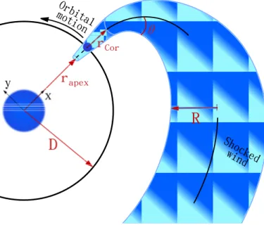
d = 3 kpc, and the inclination i is left as a free parameter. A list of the parameter values used for a generic gamma-ray binary can be found in Table1, and a sketch of the studied scenario is pre-sented in Fig.1. Throughout this section, the notation u= ||−→u ||is used to refer to a vector norm. Also, we use primed quantities in the fluid frame (FF), and unprimed ones in the frame of the star, assumed here to be the laboratory frame (LF).
2.1. Dynamics
The interaction of the stellar and the pulsar winds produces an interface region between the two where the shocked flow
apex
R
Orbital
motion
Cory
Shocked
wind
Fig. 1.Schematic zenithal view of the studied scenario (not to scale). Only a fraction of the orbit is shown for clarity.
pressures are in equilibrium: the so-called contact discontinu-ity (CD). Close to the binary system, where the orbital motion can be neglected, the shape of this surface is characterized by the pulsar-to-stellar wind momentum rate ratio, defined as η = Lp
˙ Mwvwc
(1) forΓp 1. The asymptotic half-opening angle of the CD can be
approximated by the following expression fromEichler & Usov (1993), which is in good agreement with numerical simulations (e.g.,Bogovalov et al. 2008):
θ = 28.6◦(4 − η2/5)η1/3. (2)
The apex of the CD, where the two winds collide frontally, is located along the star-pulsar direction at a distance from the star of rapex = D/(1 + √η), with D being the orbital separation. For
the adopted parameters, we obtain η = 0.018, θ = 28.7◦, and
rapex = 0.88D = 2.6 × 1012cm, the latter being constant owing
to the circularity of the orbit.
The star is located at the origin of the coordinate system, which co-rotates with the pulsar. The x-axis is defined as the star-pulsar direction, and the y-axis is perpendicular to it and points in the direction of the orbital motion. We model the evolution of the shocked stellar and pulsar winds in the inner interaction region as a straight conical structure of half-opening angle θ and increas-ing radius R, the onset of which is at x = rapex, where it has a
radius of R0= D − rapex, roughly corresponding to the
character-istic size of the CD at its apex. The shocked flows are assumed to move along the x direction in this region (i.e., the orbital velocity is neglected here with respect to the wind speed), until they reach a point where their dynamics start to be dominated by orbital effects, the Coriolis turnover. Beyond this point, the CD is pro-gressively bent in the -y direction due to the asymmetric inter-action with the stellar wind, which arises from Coriolis forces (see Fig.1for an schematic view). As a result, the shocked flow structure acquires a spiral shape at large scales. One can estimate the distance of the Coriolis turnover to the pulsar rCorby
which comes from equating the total pulsar wind pressure to the stellar wind ram pressure due to the Coriolis effect (for Γp 1):
Lp 4πcr2 Cor = ρw(D) (1+ rCor/D)2 4π T !2 r2Cor, (3)
where ρw(r) = ˙Mw/4πr2vwis the stellar wind density at a
dis-tance r from the star. Although approximate, this expression agrees well with results from 3D numerical simulations ( Bosch-Ramon et al. 2015). Numerically solving Eq. (3) for our set of parameters yields rCor = 0.94D. We note that in the case of an
elliptical system rCorchanges along the orbit.
The radiation model explained in Sect.2.2 focuses on the shocked pulsar material flowing inside the CD. The values of the Lorentz factor of this fluid are set to increase linearly with dis-tance from the CD apex (Γ0 = 1.06, v0 = c/3) to the Coriolis
turnover (Γ = 4, v = 0.97c), based on the simulations by Bogovalov et al.(2008). Beyond the Coriolis turnover, and due to some degree of mixing between the pulsar and stellar winds (see, e.g., the numerical simulations inBosch-Ramon et al. 2015), we fix the shocked pulsar wind speed vCorto a constant value that is
left as a free parameter in our model, and could account for dif-ferent levels of mixing. The shocked stellar wind that surrounds the shocked pulsar wind plays the role of a channel through which the former flows, and may have a much lower speed. This channel is assumed to effectively transfer the lateral momentum coming from the unshocked stellar wind to the shocked pulsar wind.
The trajectory of the shocked winds flowing away from the binary, which are assumed to form a (bent) conical structure, is determined by accounting for orbital motion and momen-tum balance between the upstream shocked pulsar wind and the unshocked stellar wind, with a thin shocked stellar wind channel playing the role of a mediator. This conical structure is divided into 2000 cylindrical segments of length dl = 0.05D, amount-ing to a total length of 100D. Initially, all the shocked material moves along the x axis between x = rapex and x = D + rCor.
At the latter point, its position and momentum are, in Cartesian coordinates of the co-rotating frame,
− → r = (D + rCor, 0) − → P = ( ˙Pdt, 0) , (4)
where ˙Pis the momentum rate of the shocked flow, which we estimate as:
˙ P= Lp
c · (5)
For simplicity, we are not considering the contribution of the momentum of the stellar wind loaded through mixing into the pulsar wind before the Coriolis turnover. This contribution depends on the level of mixing, and could be as high asΩ ˙Mwvw,
withΩ = R2/4(D + rCor)2 being the solid angle fraction
sub-tended by the shocked pulsar wind at the Coriolis turnover, as seen from the position of the star. We note, nonetheless, that the inclusion of the stellar wind contribution to ˙P has a mod-est impact on the radiation predictions of the model and can be neglected at this stage.
The unshocked stellar wind velocity in the co-rotating frame has components in both the x and the y directions:
− → ˆvw= vw (x, y) r + ωr (y, −x) r , (6)
where ω is the orbital angular velocity, and the hat symbol is used to distinguish ˆvw from the purely radial component of
the wind, vw. In a stationary configuration, the force that the
unshocked stellar wind exerts onto each segment of the shocked wind structure is −→ Fw= ρwˆv2wSsin α − → ˆvw ˆvw , (7)
with α being the angle between−→ˆvwand the shocked pulsar wind
velocity→−v, and S sin α = 2Rdl sin α the segment lateral sur-face normal to the stellar wind direction. The component of −→
Fwparallel to the fluid direction is assumed to be mostly
con-verted into thermal pressure, whereas the perpendicular com-ponent−F−→w⊥ =
−→
Fwsin α modifies the segment momentum
direc-tion. Thus, the interaction with the stellar wind only reorients the fluid, but it does not change its speed beyond the Coriolis turnover1.
We find the conditions for the subsequent segments by apply-ing the followapply-ing recursive relations:
− → Pi+1= − → Pi+ −−→ F⊥wdti − →v i+1= vi − → Pi Pi − → ri+1= −→ri+ −→vidti, (8)
where vi is the shocked pulsar wind velocity in each segment,
and dti = dl/vi is the segment advection time. This
proce-dure yields a fluid trajectory semi-quantitatively similar to that obtained from numerical simulations within approximately the first spiral turn (e.g.,Bosch-Ramon et al. 2015).
2.2. Characterization of the emitter
The nonthermal emission is assumed to take place in the shocked pulsar wind, which moves through the shocked stellar wind channel and follows the trajectory defined in the previous section. We consider a nonthermal particle population con-sisting only of electrons and positrons. These are radiatively more efficient than accelerated protons (e.g.,Bosch-Ramon & Khangulyan 2009), but the presence of the latter cannot be discarded. Particles are accelerated at two different regions where strong shocks develop: the pulsar wind termination shock, located here at the CD apex; and the shock that forms in the Coriolis turnover (as inZabalza et al. 2013, hereafter the Coriolis shock). In our general model, we consider for simplicity that both regions have the same power injected into nonthermal parti-cles (in the LF), taken as a fraction of the total pulsar wind lumi-nosity: LNT = ηNTLp, with ηNT = 0.1. They also have the same
acceleration efficiency ηacc= 0.1, which defines the energy gain
rate ˙Eacc0 = ηaccecB0 of particles for a given magnetic field B0.
The latter is defined through its energy density being a fraction of the total energy density at the CD apex (indicated with the subscript 0): B020 8π = ηB Lp πR2 0v0Γ 2 0 . (9)
The magnetic field is assumed toroidal, and therefore it evolves along the emitter as B0 ∝ R−1Γ−1. For simplicity, we assume
1 There must be some acceleration of the shocked flow away from the binary as a pressure gradient is expected, but for simplicity this effect is neglected here.
that all the flow particles at the Coriolis turnover are repro-cessed by the shock there, leading to a whole new population of particles. This means that the particle population beyond the Coriolis shock only depends on the properties of the latter, and is independent of the particle energy distribution coming from the initial shock at the CD apex. This assumption divides the emitter into two independent and distinct regions: one region between the CD apex and the Coriolis turnover (hereafter the inner region), and one beyond the latter (hereafter the outer region). We recall that the inner region has a velocity profile cor-responding to a linear increase inΓ, whereas in the outer region the fluid moves at a constant speed (see Sect.2.1).
To compute the particle evolution, the emitter is divided into 1000 segments of length 0.1D, in order to account for the same total length as in Sect2.1. An electron and positron population is injected at each accelerator following a power-law distribution in the energy E0, with an exponential cutoff and spectral index p: Q0(E0) ∝ E0pexp − E 0 E0max ! , (10) where E0
maxis the cutoff energy obtained by comparing the
accel-eration timescale, t0acc= E0/| ˙E0acc|, with the cooling and diffusion
timescales, t0cool = E0/| ˙E0| and t0diff = 3R02eB0/2cE0,
respec-tively (R is the perpendicular size and thus is taken R0= R). We adopt p = −2 because it allows for a substantial power to be available for gamma-ray emission. Harder, and also a bit softer electron distributions would also be reasonable options. The par-ticle injection is normalized by the total available power L0NT = LNT/Γ2. We note that E0max and L0NT are not the same for both
accelerators, since their properties differ. Particles are advected between subsequent segments following the bulk motion of the fluid (see Appendix B2 in de la Cita et al. 2016), and they cool down via adiabatic, synchrotron, and inverse Compton (IC) losses as they move along the emitter. The particle energy dis-tribution at each segment is computed in the FF following the same recursive method as in Molina & Bosch-Ramon(2018), which yields, for a given segment k:
Nk0(E0k)= N00(E00) 1 Y i=k ˙ Ei0(E0i−1) ˙ E0 i(E 0 i) , (11) where E0
kis the energy of a given particle at the location of
seg-ment k, and E0
i is the energy that this same particle had when it
was at the position of segment i, with i ≤ k (we note that E0i> E0k due to energy losses).
For every point where we have the particle distribution, the synchrotron spectral energy distribution (SED) is computed fol-lowing Pacholczyk (1970). The IC SED is obtained from the numerical prescription developed by Khangulyan et al.(2014) for a monodirectional field of stellar target photons with a black-body spectrum. The distribution of electrons is isotropic in the FF. These SEDs are then corrected by Doppler boosting and absorption processes, the latter consisting of gamma-gamma absorption with the stellar photons (e.g. Gould & Schréder 1967), and free-free absorption with the stellar wind ions (e.g., Rybicki & Lightman 1986). We do not consider emission from secondary particles generated via the interaction of gamma rays with stellar photons, although it may have a nonnegligi-ble impact on our results (see discussion in Sect. 5.2). Partial occultation of the emitter by the star is also taken into account, although it is only noticeable for very specific system-observer configurations. For a more detailed description of the SED com-putation we refer the reader toMolina et al.(2019).
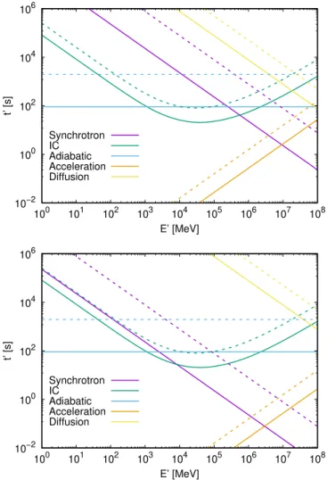
10−2 100 102 104 106 100 101 102 103 104 105 106 107 108 t’ [s] E’ [MeV] Synchrotron IC Adiabatic Acceleration Diffusion 10−2 100 102 104 106 100 101 102 103 104 105 106 107 108 t’ [s] E’ [MeV] Synchrotron IC Adiabatic Acceleration Diffusion
Fig. 2.Characteristic timescales in the FF for vCor = 3 × 10⁹, and ηB = 10−3(top panel) and 10−1(bottom panel). Solid and dashed lines represent the values at the CD apex and the Coriolis turnover locations, respectively.
3. General results
For the results presented in this section, we make use of the parameter values listed in Table1. The orbital phaseΦ is defined such that the pulsar is in the inferior conjunction (INFC) for Φ = 0, and in the superior conjunction (SUPC) for Φ = 0.5.
3.1. Energy losses and particle distribution
Figure 2 shows the characteristic timescales in the FF for the cooling, acceleration, and diffusion processes, for vCor = 3 ×
109cm s−1, and η
B= 10−3and 10−1, which correspond to initial
magnetic fields of B00= 4.15 G and 41.5 G, respectively. In gen-eral, particle cooling is dominated by adiabatic losses at the low-est energies, IC losses at intermediate energies, and synchrotron losses at the highest ones unless a very small magnetic field with ηB < 10−5 is assumed. The exact energy values at which the
different cooling processes dominate depend on ηB, and also on
whichever emitter region we are looking at. Given the depen-dency of the synchrotron and acceleration timescales on the magnetic field, and that the latter decreases linearly with dis-tance, Emax0 is higher at the Coriolis turnover than at the CD apex
(see where the synchrotron and acceleration lines intersect in Fig.2), allowing particles to reach higher energies at the location of the former. The larger region size involved and longer accu-mulation time, combined with the lower energy losses farther
1033 1034 1035 1036 1037 1038 100 101 102 103 104 105 106 107 108 E’ 2 N’(E’) [erg] E’ [MeV] ηB = 10−3 ηB = 10−1
Fig. 3.Particle energy distribution in the FF for vCor = 3 × 109cm s−1, and ηB = 10−3(green lines) and 10−1(purple lines). The contributions of the inner and outer regions are represented with dotted and dashed lines, respectively, and their sum is shown by the solid lines.
from the star, make the nonthermal particle distribution to be dominated by the outer region of the emitter, with just a small contribution from the inner part at middle energies, as seen in Fig.3(we recall that both regions are assumed to have the same injection power in the LF). The only significant effect of increas-ing the post-Coriolis shock speed to vCor = 1010cm s−1 is the
increase of the adiabatic losses by a factor of ∼3 at the Coriolis turnover location and beyond (not shown in the figures). This results in a decrease of N0(E0) for E0 . 100 MeV, where adia-batic cooling (and particle escape) dominates.
3.2. Spectral energy distribution
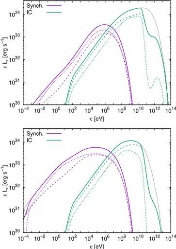
The synchrotron and IC SEDs, as seen by the observer, are shown in Figs. 4 and5 for vCor = 3 × 109cm s−1 and vCor =
1010cm s−1, respectively. We take a representative orbital phase
ofΦ = 0.3, i = 60◦, and ηB = 10−3and 10−1. The overall SED
has the typical shape for synchrotron and IC emission, with the magnetic field changing the relative intensity of each compo-nent. The IC SED is totally dominated by the outer region even if it is farther from the star and the target photon field is less dense than in the inner region. This happens because the former con-tains many more (accumulated) nonthermal particles that scatter stellar photons (see Fig. 3), and also because the ratio of syn-chrotron to IC cooling is smaller than in the inner region (there-fore, more energy is emitted in the form of IC photons at the electron energies where radiative losses dominate). Synchrotron radiation, on the other hand, is more equally distributed between the two regions. We note, however, that Doppler boosting could make the inner region dominate both the IC and synchrotron emission in a broad energy range for orbital phases close to the INFC (see Sect.3.3, and the discussion in Sect.5.1).
3.3. Orbital variability
Light curves for two different system inclinations, i = 30◦and
60◦, and post-Coriolis shock speeds, vCor = 3 × 109cm s−1and
1010cm s−1, are shown in Figs. 6 and7 for η
B = 10−3. Aside
from a change in the flux normalization, the behavior of the light curves is very similar for ηB = 10−1. The modulation of X-rays
is correlated with that of VHE gamma rays (top and bottom pan-els, respectively). Low-energy (LE) gamma rays (second panel) show a correlated modulation with VHE gamma rays and X-rays
1030 1031 1032 1033 1034 10−4 10−2 100 102 104 106 108 1010 1012 1014 ε Lε [erg s −1 ] ε [eV] Synch. IC 1030 1031 1032 1033 1034 10−4 10−2 100 102 104 106 108 1010 1012 1014 ε Lε [erg s −1 ] ε [eV] Synch. IC
Fig. 4.Observer synchrotron (purple lines) and IC (green lines) spectral energy distributions forΦ = 0.3, vCor = 3 × 109cm s−1, i = 60◦, and ηB= 10−3(top panel) and 10−1(bottom panel). The contributions of the inner and outer regions are represented with dotted and dashed lines, respectively. The black dotted lines show the total unabsorbed emission.
for vCor = 1010cm s−1, and an anti-correlated one for vCor =
3 × 109cm s−1. This change in the LE gamma-ray modulation is caused by a higher boosting (deboosting) of the outer region emission close to the INFC (SUPC) for vCor = 1010cm s−1,
which overcomes the intrinsic IC modulation. This same effect is responsible for high-energy (HE) gamma rays (third panel) to not show a clear correlation with other energy bands at high vCor, whereas they are anti-correlated with VHE gamma rays and
X-rays (and correlated with LE gamma rays) at low vCor. The
fact that Doppler boosting modulates the emission in the oppo-site way as IC does also cause the predicted variability in the inner region as seen by the observer to significantly decrease with respect to its intrinsic one, whereas the effect on the outer region is less extreme due to a lower fluid speed. Asymmetries can be observed in the light curves due to the spiral trajectory of the emitter, although they are mild because most of the radia-tion is emitted within a distance of a few orbital separaradia-tions from the star, where the spiral pattern is just beginning to form. The asymmetry only becomes more noticeable for HE gamma rays, i= 60◦, and vCor= 1010cm s−1(third panel in Fig.7), in which a
double peak structure can be seen. The proximity to the star also makes VHE emission close to the SUPC to be almost suppressed by gamma-gamma absorption.
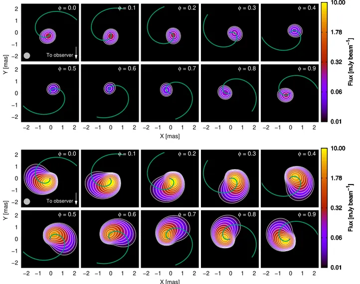
Figures 8 and 9 show, for i = 30◦ and 60◦ respectively,
simulated radio sky maps at 5 GHz for vCor = 3 × 109cm s−1,
1030 1031 1032 1033 1034 10−4 10−2 100 102 104 106 108 1010 1012 1014 ε Lε [erg s −1 ] ε [eV] Synch. IC 1030 1031 1032 1033 1034 10−4 10−2 100 102 104 106 108 1010 1012 1014 ε Lε [erg s −1 ] ε [eV] Synch. IC
Fig. 5.Same as in Fig.4, but for vCor= 1010cm s−1.
projected emission of each segment with a 2D Gaussian with increasing width to approximately simulate the segment perpen-dicular extension. The resulting maps are then convolved again with a Gaussian telescope beam of full width at half maximum (FWHM)= 0.5 mas. The contours are chosen so that the outer-most one is 10 µJy beam−1, on the order of the sensitivity of very-long-baseline interferometry (VLBI). Due to free-free absorp-tion, radio emission from the inner region is highly suppressed, and what can be seen in the sky maps comes mostly from the outer region. In particular, the part of the outer region that con-tributes most to the radio emission is located close to the Coriolis shock, and has an angular size of ∼0.5 mas, which corresponds to a linear size of ∼1 AU at the assumed distance of 3 kpc. For high ηB and the assumed angular resolution, the initial part of
the spiral structure can be traced in the radio images, especially for low inclinations. For small ηB, only the sites very close to
the Coriolis shock contribute to the emission due to the low syn-chrotron efficiency farther away, and hints of a spiral outflow cannot be seen. Regardless of the magnetic field value, the posi-tion of the maximum of the radio emission shifts for as much as ≈1 mas at different orbital phases.
4. Application to LS 5039
LS 5039 is a widely studied binary system hosting a main sequence O-type star and a compact companion, the nature of which is still unclear. Low system inclinations (i. 40◦) favor a
black hole scenario, whereas higher inclinations favor the com-pact object to be a neutron star. Inclinations above ≈60◦ are
1 2 3 4 5 1−10 keV 3 6 9 12 Flux [10 −12 erg cm −2 s −1 ] 10−30 MeV 20 40 60 80 0.1−10 GeV 0 10 20 30 0.0 0.2 0.4 0.6 0.8 1.0 1.2 1.4 1.6 1.8 2.0 φ 0.2−5 TeV
Fig. 6.Light curves at different energy ranges (indicated in the right side) for ηB= 10−3, vCor= 3×109cm s−1, and i= 30◦(purple lines) and 60◦
(green lines). The contributions from the inner and outer regions are shown with dotted and dashed lines, respectively. The vertical dot-ted blue and red lines show the position of the superior and inferior conjunctions, respectively. Two orbits are represented for a better visu-alization. 1 2 3 4 5 1−10 keV 3 6 9 12 Flux [10 −12 erg cm −2 s −1 ] 10−30 MeV 20 40 60 80 0.1−10 GeV 0 10 20 30 0.0 0.2 0.4 0.6 0.8 1.0 1.2 1.4 1.6 1.8 2.0 φ 0.2−5 TeV
Fig. 7.Same as in Fig.6, but for vCor= 1010cm s−1.
unlikely due to the absence of X-ray eclipses in this system (Casares et al. 2005). LS 5039 has an elliptical orbit with a semi-major axis of a ≈ 2.4×1012cm, an eccentricity of e= 0.35±0.04,
and a period of T ≈ 3.9 days. The superior and inferior conjunctions are located atΦ = 0.058 and 0.716, respectively, with Φ = 0 corresponding to the periastron. The star has a
−2 −1 0 1 2 Y [mas] 0.01 0.06 0.32 1.78 10.00
Flux [mJy beam
−1 ] To observer φ = 0.0 0.01 0.06 0.32 1.78 10.00
Flux [mJy beam
−1 ] φ = 0.1 0.01 0.06 0.32 1.78 10.00
Flux [mJy beam
−1 ] φ = 0.2 0.01 0.06 0.32 1.78 10.00
Flux [mJy beam
−1 ] φ = 0.3 0.01 0.06 0.32 1.78 10.00
Flux [mJy beam
−1 ] φ = 0.4 −2 −1 0 1 2 −2 −1 0 1 2 0.01 0.06 0.32 1.78 10.00
Flux [mJy beam
−1 ] φ = 0.5 −2 −1 0 1 2 0.01 0.06 0.32 1.78 10.00
Flux [mJy beam
−1 ] φ = 0.6 −2 −1 0 1 2 X [mas] 0.01 0.06 0.32 1.78 10.00
Flux [mJy beam
−1 ] φ = 0.7 −2 −1 0 1 2 0.01 0.06 0.32 1.78 10.00
Flux [mJy beam
−1 ] φ = 0.8 −2 −1 0 1 2 0.01 0.06 0.32 1.78 10.00
Flux [mJy beam
−1 ] φ = 0.9 −2 −1 0 1 2 Y [mas] 0.01 0.06 0.32 1.78 10.00
Flux [mJy beam
−1 ] To observer φ = 0.0 0.01 0.06 0.32 1.78 10.00
Flux [mJy beam
−1 ] φ = 0.1 0.01 0.06 0.32 1.78 10.00
Flux [mJy beam
−1 ] φ = 0.2 0.01 0.06 0.32 1.78 10.00
Flux [mJy beam
−1 ] φ = 0.3 0.01 0.06 0.32 1.78 10.00
Flux [mJy beam
−1 ] φ = 0.4 −2 −1 0 1 2 −2 −1 0 1 2 0.01 0.06 0.32 1.78 10.00
Flux [mJy beam
−1 ] φ = 0.5 −2 −1 0 1 2 0.01 0.06 0.32 1.78 10.00
Flux [mJy beam
−1 ] φ = 0.6 −2 −1 0 1 2 X [mas] 0.01 0.06 0.32 1.78 10.00
Flux [mJy beam
−1 ] φ = 0.7 −2 −1 0 1 2 0.01 0.06 0.32 1.78 10.00
Flux [mJy beam
−1 ] φ = 0.8 −2 −1 0 1 2 0.01 0.06 0.32 1.78 10.00
Flux [mJy beam
−1
]
φ = 0.9
Fig. 8.Simulated radio sky maps at 5 GHz for different orbital phases, vCor = 3 × 109cm s−1, i = 30◦, and ηB = 10−3 (top panel) and 10−1 (bottom panel). The assumed telescope beam is shown as a gray circle in the bottom left corner of the first plot. The contour lines start at a flux of 10 µJy beam−1and increase with a factor of 2. The star is represented (to scale) with a blue circle at (0,0), and the solid green line shows the axis of the conical emitter, the onset of which points toward the observer forΦ = 0, and opposite to it for Φ = 0.5.
luminosity of L?= (7 ± 1) × 1038erg s−1, a radius of R?= 9.3 ±
0.7 R , and an effective temperature of T?= (3.9 ± 0.2) × 104K
(Casares et al. 2005). The stellar mass-loss rate obtained through Hα measurements is in the range ˙Mw= 3.7−4.8 × 10⁻⁷M yr−1
(Sarty et al. 2011), although this value would be overestimated if the wind were clumpy (e.g.,Muijres et al. 2011). The assumption of an extended X-ray emitter (as it is the case in this work) places an upper limit for ˙Mwof up to a few times 10−7M yr−1, with
the exact value depending on the system parameters (Szostek & Dubus 2011; see also Bosch-Ramon et al. 2007). The lack of thermal X-rays in the shocked stellar wind, in the context of a semi-analytical model of the shocked wind structure, puts an upper limit in the putative pulsar spin down luminosity of Lp≤ 6 × 1036erg s−1(Zabalza et al. 2011). The latest Gaia DR2
parallax data (Gaia Collaboration 2018;Luri et al. 2018) sets a distance to the source of d= 2.1 ± 0.2 kpc. The rest of the model parameters are unknown for LS 5039.
Carrying out a statistical analysis is hardly possible in our context, as we have many free parameters or parameters that are loosely constrained. Thus, we have looked for a set of parame-ter values that approximately reproduce the observational data, but the result should be considered just as illustrative of the model capability to reproduce the source behavior, and not a
fit. We note that, for this purpose, we use a different value of the nonthermal power fraction for each accelerator (ηA
NT for the
CD apex, and ηBNT for the Coriolis shock). Table 2 shows all the model parameters used for the study of LS 5039, which are left constant throughout the whole orbit. For these parameters, we obtain η = 0.035, θ = 35.5◦, 0.55a ≤ rapex ≤ 1.14a, and
1.03a ≤ rCor≤ 1.29a, with the lower (upper) limits
correspond-ing to the periastron (apastron).
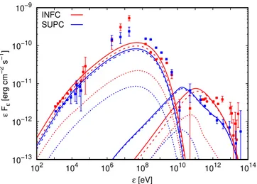
Figure10shows, for i = 60◦, the computed SED averaged
over two wide phase intervals, one around the INFC (0.45 < Φ ≤ 0.90), and the other one around the SUPC (0.90 < Φ or Φ ≤ 0.45). Observational data points of Suzaku (Takahashi et al. 2009), COMPTEL (Collmar & Zhang 2014), Fermi/LAT (Fermi LAT Collaboration 2009; Hadasch et al. 2012), and H.E.S.S. (Aharonian et al. 2006) averaged over the same phase inter-vals are also plotted. The SEDs for different system inclina-tions in which a pulsar scenario is viable (40◦ . i . 60◦) are not represented due their similarity to the one shown in Fig.10. Synchrotron emission dominates for ε . 10 GeV, with IC only contributing significantly at VHE. With the excep-tion of the COMPTEL energies (1 MeV. ε . 30 MeV), the SED reproduces reasonably well the magnitude of the observed fluxes, especially for X-rays and VHE gamma rays. At energies
−2 −1 0 1 2 Y [mas] 0.01 0.06 0.32 1.78 10.00
Flux [mJy beam
−1 ] To observer φ = 0.0 0.01 0.06 0.32 1.78 10.00
Flux [mJy beam
−1 ] φ = 0.1 0.01 0.06 0.32 1.78 10.00
Flux [mJy beam
−1 ] φ = 0.2 0.01 0.06 0.32 1.78 10.00
Flux [mJy beam
−1 ] φ = 0.3 0.01 0.06 0.32 1.78 10.00
Flux [mJy beam
−1 ] φ = 0.4 −2 −1 0 1 2 −2 −1 0 1 2 0.01 0.06 0.32 1.78 10.00
Flux [mJy beam
−1 ] φ = 0.5 −2 −1 0 1 2 0.01 0.06 0.32 1.78 10.00
Flux [mJy beam
−1 ] φ = 0.6 −2 −1 0 1 2 X [mas] 0.01 0.06 0.32 1.78 10.00
Flux [mJy beam
−1 ] φ = 0.7 −2 −1 0 1 2 0.01 0.06 0.32 1.78 10.00
Flux [mJy beam
−1 ] φ = 0.8 −2 −1 0 1 2 0.01 0.06 0.32 1.78 10.00
Flux [mJy beam
−1 ] φ = 0.9 −2 −1 0 1 2 Y [mas] 0.01 0.06 0.32 1.78 10.00
Flux [mJy beam
−1 ] To observer φ = 0.0 0.01 0.06 0.32 1.78 10.00
Flux [mJy beam
−1 ] φ = 0.1 0.01 0.06 0.32 1.78 10.00
Flux [mJy beam
−1 ] φ = 0.2 0.01 0.06 0.32 1.78 10.00
Flux [mJy beam
−1 ] φ = 0.3 0.01 0.06 0.32 1.78 10.00
Flux [mJy beam
−1 ] φ = 0.4 −2 −1 0 1 2 −2 −1 0 1 2 0.01 0.06 0.32 1.78 10.00
Flux [mJy beam
−1 ] φ = 0.5 −2 −1 0 1 2 0.01 0.06 0.32 1.78 10.00
Flux [mJy beam
−1 ] φ = 0.6 −2 −1 0 1 2 X [mas] 0.01 0.06 0.32 1.78 10.00
Flux [mJy beam
−1 ] φ = 0.7 −2 −1 0 1 2 0.01 0.06 0.32 1.78 10.00
Flux [mJy beam
−1 ] φ = 0.8 −2 −1 0 1 2 0.01 0.06 0.32 1.78 10.00
Flux [mJy beam
−1
]
φ = 0.9
Fig. 9.Same as in Fig.8, but for i= 60◦ .
of 100 MeV. ε . 10 GeV, the model overpredicts (underpre-dicts) the emission around INFC (SUPC). The hard electron spectrum allows the IC component not to strongly overestimate the fluxes around 10 GeV, although we must note that IC emis-sion from secondary pairs, not taken into account, may increase a bit the predicted fluxes.
The computed LS 5039 light curves are shown in Fig.11for the limits of the system inclination range allowed for a pulsar binary system (40◦ . i . 60◦). Most of the emission comes
from the outer region, regardless of the energy range. As in the SED, the model matches well the Suzaku and H.E.S.S observa-tions, except for an underestimation of the latter fluxes around the SUPC. Inclinations close to 60◦are favored by the presence
of a double peak in the VHE fluxes, which is not reproduced for lower values of i. This double peak is originated by the effect of the system orientation in the IC emission and Doppler boosting; the peak at Φ ≈ 0.5 has a higher intrinsic IC emission, but a lower boosting than the peak atΦ ≈ 0.85. At Fermi/LAT ener-gies, the model predicts a maximum in the light curve around the INFC and a minimum around the SUPC, contrary to what is observed. This happens because, in this energy range, the model emission is dominated by synchrotron radiation, which has a maximum around the INFC due to Doppler boosting. In the COMPTEL energy range, the relative behavior of the computed light curve is similar to the observations, although a factor of 4–5 lower.
Table 2. Parameters used for the study of LS 5039.
Parameter Value
Star Temperature T? 4 × 10⁴K
Luminosity L? 7 × 1038erg s−1 Mass-loss rate ˙Mw 1.5 × 10⁻⁷M yr−1
Wind speed vw 3 × 108cm s−1
Pulsar Luminosity Lp 3 × 1036erg s−1
Wind Lorentz factorΓp 105
System Orbit semi-major axis a 2.4 × 1012cm Orbital period T 3.9 days Orbital eccentricity e 0.35 Distance to the observer d 2.1 kpc
CD apex NT fraction ηA
NT 0.03
Cor. shock NT fraction ηB
NT 0.18
Acceleration efficiency ηacc 0.8
Injection power-law index p −1.3 Coriolis turnover speed vCor 3 × 109cm s−1
Magnetic fraction ηB 0.02
System inclination i 40◦, 60◦
Figure12shows the computed radio sky map of LS 5039 at 5 GHz, for i= 60◦and a telescope beam with FW H M= 0.5 mas.
10−13 10−12 10−11 10−10 10−9 102 104 106 108 1010 1012 1014 ε Fε [erg cm −2 s −1 ] ε [eV] INFC SUPC
Fig. 10.Observer synchrotron and IC SEDs of LS 5039 for i = 60◦ , averaged over the INFC (red lines; 0.45 < Φ ≤ 0.90) and SUPC (blue lines; 0.90 <Φ or Φ ≤ 0.45) phase intervals. Dotted and dashed lines represent the contributions of the inner and outer regions, respec-tively. From left to right, data from Suzaku, COMPTEL, Fermi/LAT, and H.E.S.S. are also represented.
The sky map for i= 40◦is very similar and is not shown. Since we do not consider particle reacceleration beyond the Coriolis shock, these maps show the synchrotron emission up to a few orbital separations from the latter, as farther away synchrotron emission is too weak to significantly contribute to the radio flux. This lack of reacceleration does not allow for a meaningful com-parison between our model and the observations. While the pre-dicted total radio flux at 5 GHz, averaged over a whole orbit, is 0.10 mJy, the detected one is around 20 mJy (Moldón et al. 2012). The assumption of a hard particle spectrum (p = −1.3) needed to explain the SEDs makes most of the available power to go into the most energetic electrons and positrons. There-fore, only a small part of the energy budget goes to those lower energy particles responsible for the radio emission, which makes the latter considerably fainter than in the generic case studied in Sect.3, in which p= −2. Despite the almost point-like and faint nature of the radio source, the emission maximum is displaced along the orbit by a similar angular distance of ≈1 mas.
5. Summary and discussion
We have developed a semi-analytical model, consisting of a 1D emitter, which can be used to describe both the dynamics and the radiation of gamma-ray binaries in a colliding wind scenario that includes orbital motion. In the following, we discuss the obtained results for a generic system and for the specific case of LS 5039, as well as the main sources of uncertainty.
5.1. General case
In general, a favorable combination of nonradiative and radia-tive losses, and residence time of the emitting particles, leads to an outer emitting region that is more prominent in its nonther-mal energy content and emission than the inner region. Thus, the SEDs are dominated by the outer region for most orbital phases. Moreover, both radio and VHE gamma-ray emission are suppressed close to the star due to free-free and gamma-gamma absorption, respectively, unless small system inclinations i < 30◦ and/or orbital phases close to the INFC are considered. Nev-ertheless, the light curves show a nonnegligible or even dom-inant contribution of the inner region close to the INFC for a
3 6 9 12 10 −12 erg cm −2 s −1 i = 40° i = 60° 1−10 keV 5 10 15 20 25 30 10 −6 ph cm −2 s −1 10−30 MeV 0.3 0.6 0.9 1.2 1.5 10 −6 ph cm −2 s −1 0.1−10 GeV 3 6 9 12 15 0.0 0.2 0.4 0.6 0.8 1.0 1.2 1.4 1.6 1.8 2.0 10 −12 erg cm −2 s −1 φ 0.2−5 TeV
Fig. 11.From top to bottom: light curves of LS 5039 in the Suzaku (1–10 keV), COMPTEL (10–30 MeV), Fermi/LAT (0.1–10 GeV), and H.E.S.S. (0.2–5 TeV) energy ranges, for i= 40◦
(purple lines) and 60◦ (green lines). The contributions of the inner and outer regions are shown with dotted and dashed lines, respectively. The phases corresponding to the INFC (SUPC) are shown with red (blue) vertical dashed lines. Flux units are not the same for all the plots.
broad energy range. This is mainly caused by the inner region emission being more Doppler-boosted than the outer region one, due to the flow moving faster in the former. Higher values of vCor(which could indicate a lower degree of mixing of stellar
and pulsar winds) tend to decrease the radiative output of the outer region due to an increase in the adiabatic losses and in the escape rate of particles from the relevant emitting region. This trend is only broken for orbital phases close to the INFC, where a higher Doppler boosting is able to compensate for the decrease of intrinsic emission in the outer region. Doppler boosting (and hence the adopted velocity profile) has also a high influence on the orbital modulation of the IC radiation in both the inner and outer regions, to the point that emission peaks can become val-leys owing to a change in the fluid speed of a factor of ∼3 in the outer region2.
Radio emission could be used to track part of the spiral tra-jectory of the shocked flow for strong enough magnetic fields with ηB & 0.1, while no evidence of such spiral structure is
pre-dicted for low fields. In any case, as long as the overall radio emission is detectable, variations of the image centroid position on the order of 1 mas (for a distance to the source of ∼3 kpc) could be used as an indication of the dependency of the emitter structure with the orbital phase. This behavior is not exclusive
2 A similar effect is expected to happen if different velocity profiles are assumed for the inner region, but this has not been explicitly explored in this work.
−2 −1 0 1 2 Y [mas] 0.010 0.014 0.020 0.028 0.040
Flux [mJy beam
−1 ] To observer φ = 0.0 0.010 0.014 0.020 0.028 0.040
Flux [mJy beam
−1 ] φ = 0.1 0.010 0.014 0.020 0.028 0.040
Flux [mJy beam
−1 ] φ = 0.2 0.010 0.014 0.020 0.028 0.040
Flux [mJy beam
−1 ] φ = 0.3 0.010 0.014 0.020 0.028 0.040
Flux [mJy beam
−1 ] φ = 0.4 −2 −1 0 1 2 −2 −1 0 1 2 0.010 0.014 0.020 0.028 0.040
Flux [mJy beam
−1 ] φ = 0.5 −2 −1 0 1 2 0.010 0.014 0.020 0.028 0.040
Flux [mJy beam
−1 ] φ = 0.6 −2 −1 0 1 2 X [mas] 0.010 0.014 0.020 0.028 0.040
Flux [mJy beam
−1 ] φ = 0.7 −2 −1 0 1 2 0.010 0.014 0.020 0.028 0.040
Flux [mJy beam
−1 ] φ = 0.8 −2 −1 0 1 2 0.010 0.014 0.020 0.028 0.040
Flux [mJy beam
−1
]
φ = 0.9
Fig. 12.Same as in Fig.9, but for the LS 5039 model parameters, with i= 60◦
. Note the change in the color scale.
of a colliding wind scenario, however, since the jets in a micro-quasar scenario could be affected by orbital motion in a simi-lar manner (e.g.,Bosch-Ramon 2013;Molina & Bosch-Ramon 2018;Molina et al. 2019).
There are some limitations in our model that should be acknowledged. One of them is the simplified dynamical treat-ment of the emitter, considered as a 1D structure. Not using proper hydrodynamical simulations makes the computed trajec-tory approximately valid within the first spiral turn, after which strong instabilities would significantly affect the fluid propaga-tion, as seen inBosch-Ramon et al.(2015). Nonetheless, since most of the emission comes from the regions close to the binary system, we do not expect strong variations in the radiative out-put due to this issue. We are not considering particle reacceler-ation beyond the Coriolis shock, although additional shocks and turbulence are expected to develop under the conditions present farther downstream (Bosch-Ramon et al. 2015), and these pro-cesses could contribute to increase the nonthermal particle ener-getics. Accounting for reacceleration would in turn increase the emission farther from the binary system, resulting for instance in more extended radio structures, although with the aforemen-tioned inaccuracies in the trajectory computation gaining more importance.
Finally, we note that the model results for a generic case could change significantly for different values of some param-eters that are difficult to determine accurately. The fluid speed and detailed geometry in the inner and outer regions are hard to constrain observationally. Precise values of the magnetic field, the electron injection index, the acceleration efficiency, and the nonthermal luminosity fraction are also difficult to obtain due to the presence of some degeneracy among them. Any significant changes in these quantities with respect to the values adopted in this work could have a strong influence on the emission outputs of the system.
5.2. LS 5039
Several model parameters can be fixed for the study of LS 5039 thanks to the existing observations of the source. Those param-eters that cannot be obtained from observations are deter-mined by heuristically (although quite thoroughly) exploring the
parameter space, trying to better reproduce the observed LS 5039 emission. For this purpose, a hard particle spectrum is injected at both accelerators, with a power-law index p= −1.3, and a very high acceleration efficiency of ηacc= 0.8 is assumed in both
loca-tions (we note that values between 0.5 and 1 give qualitatively similar results). These values are higher than those used for the general case, already quite extreme, although they cannot be dis-carded given the current lack of knowledge on the acceleration processes taking place in LS 5039 (or even the emitting pro-cess; see, e.g.,Khangulyan et al. 2020, for an alternative origin of the gamma rays in which a synchrotron-related mechanism does play a role). Additionally, since the outer region behavior reproduces better the observed (X-ray and VHE) light curves, a higher ηNT is assumed for the Coriolis shock than for the CD
apex, providing the former with a larger nonthermal luminosity budget (i.e., ηNT= 0.18 versus 0.03).
The model nicely reproduces the observed X-ray and VHE gamma-ray emission of LS 5039, as well as the HE gamma-ray flux, although it fails to properly account for the HE gamma-ray modulation due to the synchrotron dominance in this energy range. A possible solution to this issue could be the inclusion of particle reacceleration beyond the Coriolis shock, which com-bined with the lower magnetic field may result in enough IC emission to explain the observed modulation of the HE gamma rays. This would also alleviate the extreme value of ηaccneeded
for the synchrotron emission to reach GeV energies. The largest difference between the model predictions and the observations comes at photon energies around 10 MeV, where the emission is underestimated by a factor of up to 5 (although interestingly the modulation is as observed). Some MeV flux would be added if we accounted for the synchrotron emission of electron-positron pairs created by gamma rays interacting with stellar photons (e.g.,Bosch-Ramon et al. 2008;Cerutti et al. 2010), which is not included in our model. However, this component cannot be much larger than the TeV emission, as otherwise IC from these sec-ondary particles would largely violate the 10 GeV observational flux constraints. Therefore, the energy budget of secondaries alone cannot explain the MeV flux.
The lack of predicted VHE emission around the SUPC is due to strong gamma-gamma absorption. The fact that we use a 1D emitter at the symmetry axis of the conical CD overestimates
this absorption, since we are not considering emitting sites at the CD itself, which is approximately at a distance R from the axis (see Fig. 1) or even farther (see the shocked pulsar wind extension in the direction normal to the orbital plane in the cor-responding maps in Bosch-Ramon et al. 2015). Within a few orbital separations from the pulsar (where most of the emission comes from), the CD is significantly farther from the star than its axis, and the observer, star, and flow relative positions are also quite different, allowing for lower absorption in some of the emitting regions. Therefore, the use of an extended emit-ter would reduce gamma-gamma absorption and increase the predicted VHE fluxes around the SUPC, possibly explaining the H.E.S.S. fluxes. Particle reacceleration beyond the Coriolis shock may also make some regions farther away from the star to emit VHE photons that would be less absorbed. As already dis-cussed for the general case, reacceleration would also extend the radio emission and, if accounted for, could allow for a sky map comparison with VLBI observations (e.g.,Moldón et al. 2012). Thus, one could constrain a reacceleration region added to our model using VLBI observations, but this is beyond the scope of the present work. It is worth noting that emission from sec-ondary particles could also have a significant contribution to the extended and nonextended VLBI components (Bosch-Ramon & Khangulyan 2011).
Our computed SED is qualitatively different to the best fit scenario presented indel Palacio et al.(2015), in which a one-zone model was applied for an accelerator in a fixed position at a distance of 1.4a ≈ 3.3 × 1012cm from the star. Although the
general shape is similar, their SED is totally dominated by IC down to ∼1 MeV, whereas in our model IC is only relevant at energies&10 GeV. Another one-zone model inTakahashi et al. (2009) explains well the X-ray and VHE gamma-ray emission and modulation, although it underestimates the fluxes at MeV and GeV energies (which were not available by the time of pub-lication of this work). Our synchrotron and IC phase-averaged SEDs above 100 MeV are somewhat close to those in Zabalza et al.(2013). They applied a two-zone model to LS 5039, with the two emitting regions located at the CD apex and the Cori-olis shock. Their model reproduces better the GeV modulation, although it also fails to explain the MeV emission, and under-estimates the X-ray emission by more than one order of magni-tude. Similar results were obtained byDubus et al.(2015) with a model that computes the flow evolution through a 3D hydro-dynamical simulation of the shocked wind close to the binary system, where orbital motion is still unimportant (and thus, it does not include the Coriolis shock). Modulation in the HE band is well explained there, although both the X-ray and the MeV emission are underestimated. All of the above, added to the fact that the 1D emitter model presented in this work also fails to reproduce some of the LS 5039 features, seems to point toward the need of more complex models to describe the behavior of this source, accounting for particle reacceleration, using data from 3D (magneto-)hydrodynamical simulations to compute the evolution of an emitter affected by orbital motion, and possibly including the unshocked pulsar wind zone to correctly describe the MeV radiation (see, e.g.,Derishev et al. 2012).
Acknowledgements. We would like to thank the referee for his/her construc-tive and useful comments, which were helpful to improve the manuscript. We acknowledge support by the Spanish Ministerio de Economía y Competitivi-dad (MINECO/FEDER, UE) under grant AYA2016-76012-C3-1-P, with par-tial support by the European Regional Development Fund (ERDF/FEDER), and from the Catalan DEC grant 2017 SGR 643. EM acknowledges support from MINECO through grant BES-2016-076342.
References
Abeysekara, A. U., Benbow, W., Bird, R., et al. 2018,ApJ, 867, L19
Aharonian, F., Akhperjanian, A. G., Aye, K. M., et al. 2005,A&A, 442, 1
Aharonian, F., Akhperjanian, A. G., Bazer-Bachi, A. R., et al. 2006,A&A, 460, 743
Aharonian, F. A., Akhperjanian, A. G., Bazer-Bachi, A. R., et al. 2007,A&A, 469, L1
Barkov, M. V., & Bosch-Ramon, V. 2016,MNRAS, 456, L64
Bogovalov, S. V., Khangulyan, D. V., Koldoba, A. V., Ustyugova, G. V., & Aharonian, F. A. 2008,MNRAS, 387, 63
Bosch-Ramon, V. 2013,Eur. Phys. J. Web Conf., 61, 03001
Bosch-Ramon, V., & Barkov, M. V. 2011,A&A, 535, A20
Bosch-Ramon, V., & Khangulyan, D. 2009,Int. J. Mod. Phys. D, 18, 347
Bosch-Ramon, V., & Khangulyan, D. 2011,PASJ, 63, 1023
Bosch-Ramon, V., Motch, C., Ribó, M., et al. 2007,A&A, 473, 545
Bosch-Ramon, V., Khangulyan, D., & Aharonian, F. A. 2008,A&A, 482, 397
Bosch-Ramon, V., Barkov, M. V., Khangulyan, D., & Perucho, M. 2012,A&A, 544, A59
Bosch-Ramon, V., Barkov, M. V., & Perucho, M. 2015,A&A, 577, A89
Casares, J., Ribó, M., Ribas, I., et al. 2005,MNRAS, 364, 899
Cerutti, B., Malzac, J., Dubus, G., & Henri, G. 2010,A&A, 519, A81
Collmar, W., & Zhang, S. 2014,A&A, 565, A38
Corbet, R. H. D., Chomiuk, L., Coe, M. J., et al. 2016,ApJ, 829, 105
Corbet, R. H. D., Chomiuk, L., Coe, M. J., et al. 2019,ApJ, 884, 93
de la Cita, V. M., Bosch-Ramon, V., Paredes-Fortuny, X., Khangulyan, D., & Perucho, M. 2016,A&A, 591, A15
del Palacio, S., Bosch-Ramon, V., & Romero, G. E. 2015,A&A, 575, A112
Derishev, E. V., & Aharonian, F. A. 2012, in American Institute of Physics Conference Series, eds. F. A. Aharonian, W. Hofmann, & F. M. Rieger,Am. Inst. Phys. Conf. Ser., 1505, 402
Dubus, G. 2006,A&A, 456, 801
Dubus, G. 2013,A&ARv., 21, 64
Dubus, G., Lamberts, A., & Fromang, S. 2015,A&A, 581, A27
Dubus, G., Guillard, N., Petrucci, P.-O., & Martin, P. 2017,A&A, 608, A59
Eger, P., Laffon, H., Bordas, P., et al. 2016,MNRAS, 457, 1753
Eichler, D., & Usov, V. 1993,ApJ, 402, 271
Fermi LAT Collaboration (Abdo, A. A., et al.) 2009,ApJ, 706, L56
Fermi LAT Collaboration (Ackermann, M., et al.) 2012,Science, 335, 189
Gaia Collaboration (Brown, A. G. A., et al.) 2018,A&A, 616, A1
Gould, R. J., & Schréder, G. P. 1967,Phys. Rev., 155, 1408
Hadasch, D., Torres, D. F., Tanaka, T., et al. 2012,ApJ, 749, 54
Hess, C., Abramowski, A., et al. 2015,MNRAS, 446, 1163
Hinton, J. A., Skilton, J. L., Funk, S., et al. 2009,ApJ, 690, L101
Khangulyan, D., Hnatic, S., Aharonian, F., & Bogovalov, S. 2007,MNRAS, 380, 320
Khangulyan, D., Aharonian, F. A., & Kelner, S. R. 2014,ApJ, 783, 100
Khangulyan, D., Aharonian, F., Romoli, C., & Taylor, A. 2020, ArXiv e-prints [arXiv:2003.00927]
Leahy, D. A. 2004,A&A, 413, 1019
Luri, X., Brown, A. G. A., Sarro, L. M., et al. 2018,A&A, 616, A9
Maraschi, L., & Treves, A. 1981,MNRAS, 194, 1P
Moldón, J., Ribó, M., & Paredes, J. M. 2012,A&A, 548, A103
Molina, E., & Bosch-Ramon, V. 2018,A&A, 618, A146
Molina, E., del Palacio, S., & Bosch-Ramon, V. 2019,A&A, 629, A129
Muijres, L. E., de Koter, A., Vink, J. S., et al. 2011,A&A, 526, A32
Muijres, L. E., Vink, J. S., de Koter, A., Müller, P. E., & Langer, N. 2012,A&A, 537, A37
Pacholczyk, A. G. 1970,Radio Astrophysics. Nonthermal Processes in Galactic and Extragalactic Sources(W. H. Freeman & Company)
Paredes, J. M., & Bordas, P. 2019, ArXiv e-prints [arXiv:1901.03624] Paredes, J. M., Martí, J., Ribó, M., & Massi, M. 2000,Science, 288, 2340
Pauldrach, A., Puls, J., & Kudritzki, R. P. 1986,A&A, 164, 86
Rybicki, G. B., & Lightman, A. P. 1986,Radiative Processes in Astrophysics
(Wiley-VCH)
Sarty, G. E., Szalai, T., Kiss, L. L., et al. 2011,MNRAS, 411, 1293
Sierpowska-Bartosik, A., & Torres, D. F. 2007,ApJ, 671, L145
Szostek, A., & Dubus, G. 2011,MNRAS, 411, 193
Takahashi, T., Kishishita, T., Uchiyama, Y., et al. 2009,ApJ, 697, 592
Takata, J., Leung, G. C. K., Tam, P. H. T., et al. 2014,ApJ, 790, 18
Tavani, M., Kniffen, D., Mattox, J. R., Paredes, J. M., & Foster, R. S. 1998,ApJ, 497, L89
Zabalza, V., Bosch-Ramon, V., & Paredes, J. M. 2011,ApJ, 743, 7
Zabalza, V., Bosch-Ramon, V., Aharonian, F., & Khangulyan, D. 2013,A&A, 551, A17
Zanin, R., Fernández-Barral, A., de Oña Wilhelmi, E., et al. 2016,A&A, 596, A55