Low-complexity motion estimation for the Scalable Video
Coding extension of H.264/AVC
Livio Lima
a, Daniele Alfonso
b, Luca Pezzoni
b, Riccardo Leonardi
aa
Department of Electronics for Automation, University of Brescia, Brescia, Italy
bAdvanced System Technology Labs, STMicroelectronics, Agrate Brianza, Italy
ABSTRACT
The recently standardized Scalable Video Coding(SVC) extension of H.264/AVC allows bitstream scalability with improved rate-distortion efficiency with respect to the classical Simulcasting approach, at the cost of an increased computational complexity of the encoding process. So one critical issue related to practical deployment of SVC is the complexity reduction, fundamental to use it in consumer applications. In this paper, we present a fully scalable fast motion estimation algorithm that enables an excellent complexity performance.
Keywords: Fast Motion Estimation, H.264, Scalable Video Coding
1. INTRODUCTION
Most of the activity of the ISO and ITU Joint Video Team (JVT) over the last few years has been dedi-cated to scalable video, and this work has recently seen recognition in the so called “Scalable Video Cod-ing”extension(SVC) of the H.264/AVC standard for video compression1, 2 . Contrasting from the classical video
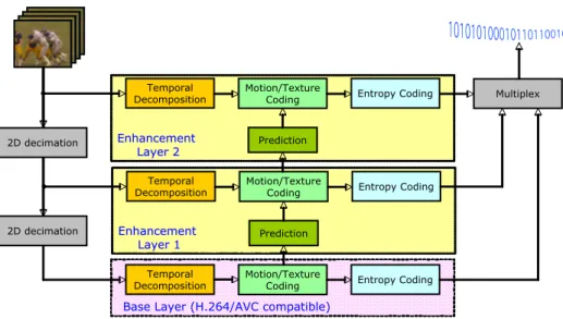
coding approach, the scalable paradigm enables the decoding from a unique coded representation(bitstream) at different “working points”in terms of spatial, quality and temporal resolution. The main drawback of the SVC architecture, shown in Figure 1, is the complexity increase compared to H.264 single layer coding. In SVC the original video sequence is downsampled to generate lower spatial resolutions that can be encoded at different quality layers. The lowest decodable point (in terms of spatial and quality resolution) is called Base Layer and is H.264/AVC compatible, while the others layers are called enhancement layers. The Inter-layer prediction is a new tool introduced in SVC that enables the reuse of the motion, texture and residual information from lower layers to improve the compression efficiency of the enhancement layers. In particular, from the motion estimation point of view, it has been shown that better compression performance are obtained by performing the full motion estimation process independently at each layer, where for the enhancement layers additional new macroblock modes(introduced by the Inter-layer prediction and defined in SVC standard) have to be evaluated. Because the motion estimation process is responsible for most of the encoding time, it is clear as this multi-layer architecture drastically increases the complexity compared to single-layer coding. This is one of the reason why the success of this scalable video coding extension will depend on the tradeoff between complexity and performance compared to the use of simulcast or transcoding solutions. A complexity analysis of the new SVC standard con be found in3 .
This work presents the full scalable extension of a fast motion estimation algorithm for the base layer and temporal scalability that was presented in4. The overall proposed algorithm not only decreases the complexity of
the motion estimation process for the enhancement layers (independently from the adopted scalability configura-tion), but it also provides a fast motion estimation algorithm for the base layer. This is the reason why different algorithms are used for motion estimation in the base layer and in the enhancement layers, as will be described in the following. The results show that the proposed algorithm could greatly decrease the complexity in terms of number of tested motion vectors with comparable compression performance to the fast motion estimation algorithm proposed in the reference software5 .
Further author information: (Send personal correspondence to Livio Lima or Daniele Alfonso) Livio Lima: E-mail: [email protected], Telephone: +390303715457
2D decimation
Temporal
Decomposition Motion/TextureCoding Entropy Coding
Multiplex
Base Layer (H.264/AVC compatible)
Base Layer (H.264/AVC compatible)
2D decimation
Prediction Temporal
Decomposition Motion/TextureCoding Entropy Coding Enhancement Enhancement Layer 1 Layer 1 Prediction Temporal
Decomposition Motion/TextureCoding Entropy Coding Enhancement
Enhancement
Layer 2
Layer 2
Figure 1. Scalable Video Coder structure
The remainder of the paper is structured as follow. Sections 2 gives a brief explanation on how the proposed algorithm works for the base layer, while in Section 3 the multi-layer extension is proposed. Finally Section 4 provides the conducted experimental simulations.
2. MOTION ESTIMATION IN BASE LAYER
The motion estimation algorithm in SVC base layer is based on two main steps: the Coarse Search and the Fine Search. The Coarse search is a pre-analysis step useful to initialize the Fine Search, which provides the motion vectors that will be used to actually encode each block.
2.1 Coarse Search
The Coarse Search is a pre-processing step that finds a single motion vector for each 16x16 macroblock of each frame following the display order and it uses only the previous original frame as reference. The Coarse Search could be applied on the whole sequence before the encoding process or independently within each Group of Picture (described in the follow). If the current macroblock is at position (i, j) in frame n, the Coarse Search tests 3 spatial predictors and 3 temporal predictors(obviously available from the second frame), where the 6 predictors are the motion vectors already computed for the Coarse Search of previous macroblocks. The spatial predictors are the vectors of the macroblocks in position (i − 1, j), (i, j − 1), (i − 1, j − 1) in frame n, while the temporal predictors are related to the macroblocks in position (i, j), (i, j−1), (i−1, j) in frame n-1. Subsequently a grid of 12 fixed motion vectors called “short updates”at half pel accuracy are added to the best spatial/temporal predictor to get the best motion vector for the 16x16 macroblock. At each step the criteria for the choice of the best motion vector is the minimization of the Sum of Absolute Differences (SAD). The vectors estimated during the Coarse Search do not have coding purposes, but are used as a good starting point for the Fine Search step explained in the next section.
It is important to note as the Coarse Search process is performed only on the input spatial resolution used to generate the base layer, that is potentially a downsampled version of the video sequence used to encode the enhancement layers, as in case of spatial scalability. It follows as the motion information generated by the Coarse Search has to be adjusted in order to be used in the Fine Search of the enhancement layers, as will be explained in section 3.
GOP border GOP border
key-pic B-lev-2 B-lev-1 B-lev-2 B-lev-0 B-lev-2 B-lev-1 B-lev-2 key-pic
f0
f1
f2
f3
f4
f5
f6
f7
f8
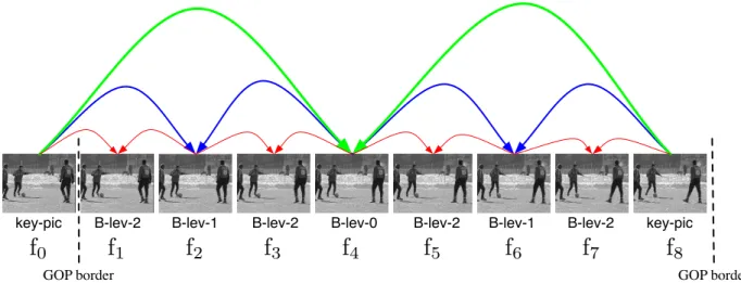
Figure 2. Hierarchical B-frame decomposition structure for a single GOP
2.2 Fine Search
The Fine Search is the step of the algorithm that is responsible for the estimation of the final motion vectors for each macro-blocks that are subsequently used for the motion compensation and coding. The Fine Search is applied on each frame following the encoding order given by the particular temporal decomposition struc-ture, where in the rest of the work only the Hierarchical B-frame decomposition, that enables native temporal scalability with improved performance compared to other structures,6 is considered. As shown in Figure 2, the
Hierarchical B-frame decomposition processes the video sequence in Group of Pictures (GOP) where for each GOP the last frame, called picture, is intra-coded(I-frame) or inter-coded(P-frame) with the previous key-picture as reference. Al the other key-pictures within the GOP are inter-coded as bidirectional key-pictures(B-frame) using the reference as shown in Figure 2. Since Hierarchical B-frame enbles the closed-loop motion estimation, during the Fine Search the motion estimation is performed using the decoded version of the reference frames.
For the understanding of the proposed algorithm, is also important to note as inside the reference software the bidirectional motion-estimation (for B-frames) for each block is not performed by joint search of the forward and backward motion vectors. First the best forward and backward vectors are independently estimated by one-directional motion estimation, then an iterative procedure “corrects”the vectors for bi-one-directional estimation. At each step of the iterative procedure one motion vector is fixed while the other one is refined. This is the reason because the Fine Search is further split in 2 steps: the one-directional step, and the bi-directional refinement. In B frames the one-directional step is applied two times to search the best forward and backward motion vectors and then the bi-directional refinement is applied, while P frames need only to the one-directional step to find the best backward motion vector.
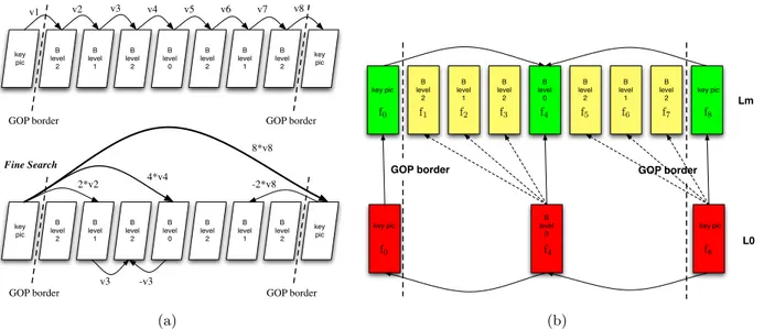
For each macroblock the one-directional step is applied for each block type because different partitioning scheme are evaluated for each macroblock. This means that the motion estimation process has to be performed for each possible sub-block(16x16, 16x8, 8x16, ...). Similarly to the Coarse Search, the Fine Search tests 3 temporal predictors and 3 spatial predictors, where the difference is in the meaning of the temporal and spatial predictors. In fact the spatial predictors are the result of the Fine Search already performed for the spatially adjacent blocks of the same size (and not macroblocks) while the temporal predictors are the results of Coarse Search scaled by an appropriate ratio, as shown in Figure 3(a).
To understand the meaning of the temporal and spatial predictors let consider the following example. Suppose to apply the one-directional step for the macroblock (i, j) of the frame f4, inspecting the macroblock mode Mx,
in order to obtain the Fine Search vectors f4,b(i, j, Mx) and f4,f(i, j, Mx). Let assume that c4(i, j) is the Coarse
Search motion vector for the macroblock (i, j) in frame f4 that has been estimated with a motion estimation
estimation is performed with respect to the previous frame. Since the temporal distance between f4 and its
references (f0and f8) is equal to 4 pictures, the temporal predictors has to be rescaled by a factor of 4. The sets
of temporal(T ) and spatial(S) predictors for backward and forward motion vectors are given by:
Tb(i, j) = {4c4(i, j), 4c4(i − 1, j), 4c4(i, j − 1)} Tf(i, j) = {−4c4(i, j), −4c4(i − 1, j), −4c4(i, j − 1)}
Sb(i, i) = {f4,b(i − 1, j − 1, Mx), f4,b(i − 1, j, Mx), f4,b(i, j − 1, Mx)}
Sf(i, i) = {f4,f(i − 1, j − 1, Mx), f4,f(i − 1, j, Mx), f4,f(i, j − 1, Mx)}
The best backward and forward predictor is choosed through a RD-optimization pb(i, j, Mx) = arg min
x∈Tb,Sb
(d(x) + λmot·r(x, bl mode Mx))
pf(i, j, Mx) = arg min
x∈Tf,Sf
(d(x) + λmot·r(x, bl mode Mx))
where d() is the MSE on the block (i, j) obtained using the vector x and r() is the cost function.
The best predictor is than refined through 3 different sets of update vectors: short(US), medium(UM) and
long(UL), where the new groups of medium and long updates are defined in order to take in account the distance
between current and reference frame in case of possibly long GOP. n particular, if D ≥ 8 long, medium and short updates are tested, if D = 4 or D = 2 medium and short updates are tested and if D = 1 only short updates are tested. So, for the above example, the best “updated backward predictor”(ub) is given by:
uMb (i, j) = pb+ arg min
u∈UM
(d(pb+ u) + λmot·r(pb+ u, bl mode Mx))
ub(i, j) = uMb + arg min
u∈US
(d(uM
b + u) + λmot·r(uMb + u, bl mode Mx))
The number and the values of the updates, as also the threshold value D are experimentally derived through an extensive set of simulations over different test sequences with different coding parameters in order to obtain the best tradeoff between performance and complexity. After the updates evaluation, for efficiency purpose ub
is compared to the zero motion vector(z) and the H.264 predictor(p264) and the best one is finally refined at quarter-pel accuracy(with vectors taken from the set UQP), in order to find the final Fine Search motion vector
f4,b(i, j, Mx) for the MB mode Mx:
ˆf4,b(i, j, Mx) = arg min
x∈{ub,z,p264}
(d(x) + λmot·r(x, bl mode Mx))
f4,b(i, j, Mx) = ˆf4,b+ arg min
u∈UQP
(d(ˆf4,b+ u) + λmot·r(ˆf4,b+ u, bl mode Mx))
The bi-directional motion vectors are obtained through an iterative refinement of one-directional vectors. At each step of the iterative procedure one motion vector is fixed while the other one is refined through 8 updates at quarter pel accuracy.
3. MULTI LAYER EXTENSION
To simplify the notation, referred to Figure 3(b) the base layer (BL) is identified by L0while a general
enhance-ment layer (EL) is represented as Lm. Exploiting the motion information from lower layers, for each picture of
higher layers we can expect to have a good representation of the motion using an appropriate scaled version of the motion flow of the corresponding pictures at lower layers. This is not true when a particular picture in a higher level has no associated picture at lower layers, for example when a different frame rate is used from one layer to another, thus a different motion estimation approach is used for pictures with or without an associated frame in lower layers. This problem is shown in Figure 3(b), where an 8-picture GOP is considered and the EL has a frame-rate 4 times larger then the BL. In this case, for the key-pictures (if P-type) and for B-level-0 pictures the motion information are directly inferred from the corresponding pictures in the BL, following the
key pic B level 2 B level 1 B level 2 B level 0 B level 2 B level 1 B level 2 key pic GOP border GOP border key pic B level 2 B level 1 B level 2 B level 0 B level 2 B level 1 B level 2 key pic GOP border GOP border v1 v2 v3 v4 v5 v6 v7 v8 2*v2 4*v4 8*v8 -2*v8 v3 -v3 Coarse Search Fine Search (a) key pic B level 2 B level 1 B level 2 B level 0 B level 2 B level 1 B level 2 key pic key pic B level 0 key pic
GOP border GOP border
L0 Lm f0 f0 f1 f2 f3 f4 f5 f6 f7 f8 f4 f8 (b)
Figure 3. 3(a): Scaling of Coarse Search motion vectors to obtain temporal predictors in Fine Search; 3(b): Motion scaling between layers with different frame-rate
process described in section 3.2. This case leads to a better compression efficiency and a speed-up of the motion estimation process. For the B-level-1 and -2 pictures the correspondence with the BL is missing, and consequently the motion information are similarly to what was used for the BL (see subsection 3.1).
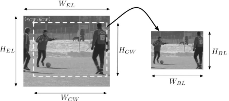
The problem of the different frame-rate is not the only aspect that has to be considered during the multi-layer extension process. In fact the SVC standard allows a particular type of spatial scalability, named Extended Spatial Scalability (ESS), where generally the BL is a scaled and cropped version of EL, as in case of SDTV to HDTV scalability, for which SDTV represents a base layer with 4:3 aspect ratio whereas HDTV corresponds to a 16:9 aspect ratio enhancement layer. The ESS defines the concept of Cropping Window (CW), that is the area of the EL used to generate the BL, as shown in Figure 4. In sections 3.1 and 3.2 we will refer as (WBL, HBL) the dimension of the BL, (WEL, HEL) the dimension of the EL, (xCW, yCW) the origin of
the CW inside the EL and with (WCW, HCW) the dimension of the CW. Obviously, depends on the value of
these quantities it corresponds a different scalability configuration. So, for eample, if (xCW, yCW) = (0, 0) and
(WCW, HCW) = (WEL, HEL) = (2WBL, 2HBL) we assume dyadic spatial scalability, if (xCW, yCW) = (0, 0) and
(WCW, HCW) = (WEL, HEL) = (WBL, HBL) is the case of CGS, and so on. This is the reason since in the
following all the algorithms will be generically presented. Therefore a layer can be of any type: CGS, MGS, dyadic spatial or ESS.
3.1 Frame without an associated match in lower layers
When the lower layers do not provide any motion information to the upper ones, the motion estimation process for the EL follows the algorithm explained in section 2 for the BL. The only difference concerns the Coarse Search, since as previously explained the full Coarse Search process is performed only for the BL. In order to have the temporal predictors for the Fine Search at higher layers, a scaling of the motion vectors obtained from the Coarse Search is performed. Hereafter, the process is explained only for one EL with respect to the BL. Similarly it could be easily extended between 2 consecutive enhancement layers. Let us define the frame rate ratio fR= fEL/fBLas the ratio between the frame rates of the EL(fEL) and BL(fBL), and the resolution ratios
as follow:
rX= WWCW
BL rY =
HCW
HBL (1)
Referred to Figure 3(b), suppose to estimate the temporal predictor c2,EL(i, j) for the macroblock (i, j) at
WBL HBL HEL WCW HCW WEL (xCW, yCW)
Figure 4. Base layer generation from Cropping Window
c4,BL(h, k) estimated for frame f4 of the BL has to be used to infer the temporal predictors. If the current macroblock lies inside the cropping window, the Coarse Search motion vectors c2,EL(i, j) for MB (i, j) in the EL
is computed as
c2,EL(i, j).x = c4,BL(h, k).x ∗ rX
fR c2,EL(i, j).y =
c4,BL(h, k).y ∗ rY
fR (2)
where h and k are the indexes of the macroblock of BL with coordinate [xBL(h, k), yBL(h, k)] of the upper-left
pixel given by:
xBL(h, k) = xEL(i, j) − xr CW
X yBL(h, k) =
yEL(i, j) − yCW
rY (3)
If the MB (i, j) lies outside the cropping window, as in the case of ESS with cropped BL, we can not use the BL motion information, and so c2,EL(i, j) = 0. After this scaling process, the Fine Search is performed as
explained in section 2.2. So, the set of temporal predictors for frame f2 in the EL, is given by:
Tb(i, j) = {2c2,EL(i, j), 2c2,EL(i, j − 1), c2,EL(i − 1, j)}
Tf(i, j) = {−2c2,EL(i, j), −2c2,EL(i, j − 1), −2c2,EL(i − 1, j)}
3.2 Frame with match in lower layers
For the pictures with corresponding low-layer representations, like KP and B0 pictures in Figure 3(b), we can fully exploit the motion information of the BL, expecting good performance with reduced computational complexity. However, these considerations are not completely true in case of ESS scalability so, in general, the reuse of the BL motion information can be done only for the blocks of the EL that lie within the cropping window. Furthermore, the performance depends also on the quality of the pictures in the BL. The higher the quality of the BL the more efficient the inter-layer prediction, both for texture and motion information. In order to show the dependencies between the quality of th BL and the performance of the proposed algorithm, two scenarios are considered:
• low complexity: the one-directional step of the Fine Search tests only 1 inter-layer predictor inferred from the lower layers (see below), together with the predicted motion vector provided by the SVC encoder and the zero motion vector. The best vector is finally refined through 8 updates at quarter pel accuracy. The bi-directional step is the same of the BL.
• high complexity: the one-directional step of the Fine Search tests 1 inter-layer predictor inferred from lower layers and refines it with short, medium and long updates as explained in section 2.2, together with the predicted motion vector provided by the SVC encoder and the zero motion vector. The best vector is finally refined through 8 updates at quarter-pel accuracy. The bi-directional step is the same of the BL.
It’s important to note as since in this case the Fine Search does not test the temporal predictors, the scaling of the Coarse Search information, described is section 3.1, is not needed.
Again, referred to Figure 3(b), let consider to estimate the one-directional inter-layer predictor (backward or forward) p4(i, j, Mx) for the macroblock (i, j) at position [xEL(i, j), yEL(i, j)] (that lies inside the Crop Window)
in frame f4 of the EL for the particular macroblock mode Mx. Each macroblock mode has a relative position
(xMx, yMx) inside the macroblock. The inter-layer predictor is a scaled version of motion vector f4,BL(h, k, Mx) computed in the Fine Search for the corresponding block mode Mx of BL where h and k are the indexes of the
macroblock of BL with coordinate [xBL(h, k), yBL(h, k)] of upper-left pixel given by the equation 3, while the
position of the block inside the macroblock is given by xBL(h, k, Mx) =xEL(i, j) − xr CW+ xMx
X yBL(h, k, Mx) =
yEL(i, j) − yCW + yMx rY
The value of the predictor is given by:
p4(i, j, Mx).x = f4,BL(h, k, Mx).x ∗ rX p4(i, j, Mx).y = f4,BL(h, k, Mx).y ∗ rY
As explained before, if the MB lies outside the cropping window, the motion information of the block is derived using the motion estimation algorithm explained in section 2, where the Fine Search is performed with zero temporal predictors.
4. EXPERIMENTAL RESULTS
In order to evaluate the performance of the proposed algorithm different configurations have been tested: Coarse Grain Scalability (CGS), Medium Grain Scalability (MGS), dyadic Spatial Scalability (SPA) and Extended Spatial Scalability (ESS), in each case using different test sequences, where the HD sequences used for ESS test are provided in7 .
In all the configurations we compare the fast search algorithm used in the JSVM 9.14 reference software8
and the proposed algorithm in terms of Rate-Distortion (R-D) performance and complexity. More details about how the fast search algorithm adopted in JSVM software works can be found in5 . The R-D performance is
evaluated using the Bjontegaard Delta9 , as suggested by the JVT commitee, while the complexity is evaluated
as the number of tested 4x4 block-match for each macroblock performed during the motion estimation process. Has been chosen to evaluate the complexity in terms of number of match in comparison to the encoding time because at the moment only software implementation of the SVC encoder are available, while the final target of our work is the hardware implementation for real-time coding. With software implementation the encoding time strongly depends on the level of optimization of the code, as for example efficient implementation of the matching functions or optimization for particular architectures. At the moment our algorithms have still to be optimized and so a comparison of the encoding time is not a fairly indicator of the complexity reduction. Furthermore, in view of an hardware implementation, the aim is to minimize the number of matching performed for each macroblock because this is the most time-consuming operation involved in the encoding process for each macroblock.
The main settings of JSVM software used for all the configuration are: 4, 8 and 16 picture GOP dimension with P-type key-picture, adaptive inter-layer prediction, single loop decoding and intra perdiod usually equal to 2 or 4 times the GOP dimension. For the SPA e ESS configurations we tested two different encoding modes for the EL: the first one using the same QP for both the BL and EL, while in the second one the QP of the EL is set to the QP of the BL - 6. In the CGS configuration we test only the case with QP of the EL is equal to QP of the BL - 6, as suggested in.8 In MGS configuration we usually define 2 enhancement layers with 3 MGS vectors
for each one and the extraction process to obtain the sub-bitstreams has been performed using the “Quality Layers”10 . In terms of resolution and frame-rate, for the SPA test we used a CIF BL at 30Hz and a 4CIF EL
at 30Hz or 60Hz; for the CGS and MGS tests both CIF 30Hz and 4CIF 30 Hz while for the ESS test we used a SDTV (720x576) BL at 25Hz and a HDTV EL (1920x1024) at 50 Hz. At the moment, the proposed algorithm supports only the progressive mode, and so the SDTV BL used in ESS experiments is not a native PAL/NTSC format, but rather it was obtained by cropping and downsampling the original HDTV video. For the dyadic
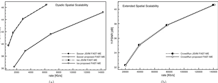
2000 4000 6000 8000 10000 12000 14000 rate [Kb/s] 36 38 40 42 44 46 Y -PSNR [dB] Soccer JSVM FAST-ME Soccer proposed FAST-ME Ice JSVM FAST-ME Ice proposed FAST-ME
Dyadic Spatial Scalability
(a) 20000 40000 60000 80000 100000 120000 140000 rate [Kb/s] 32 34 36 38 40 Y -PSNR [dB] CrowdRun JSVM FAST-ME CrowdRun proposed FAST-ME
Extended Spatial Scalability
(b)
Figure 5. 5(a): RD comparison for SPA using a GOP size = 8; 5(b): RD comparison for ESS using a GOP size = 8
5000 10000 15000 20000 25000 rate [Kb/s] 34 36 38 40 42 44 Y -PSNR [dB] Harbour JSVM FAST-ME Harbour proposed FAST-ME
Coarse Grain Scalability
(a) 5000 10000 15000 20000 25000 rate [Kb/s] 34 36 38 40 42 44 Y -PSNR [dB] Harbour JSVM FAST-ME Harbour proposed FAST-ME
Coarse Grain Scalability
(b)
Figure 6. 6(a): RD comparison for CGS using a GOP size = 8; 6(b): RD comparison for MGS using a GOP size = 8 and Extended Spatial Scalability simulations we used the high complexity version of the algorithm, because the different spatial format decrease the inter-layer correlation between the respective motion fields, requiring a more accurate motion estimation in the EL. In CGS and MGS, the low complexity mode of the algorithm has been used because each layer has the same resolution and it is reasonable that the EL needs only a refinement of the BL layer motion information. Therefore fewer motion vectors estimation should provide for enough quality improvement.
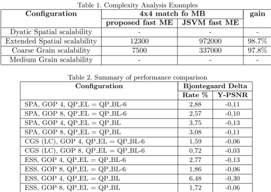
Examples of R-D comparison for SPA, ESS, CGS and MGS configurations are shown in Figure 5(a), 5(b), 6(a) and 6(b), while Table 1 presents the mean number of 4x4 block-match for MB for these configurations. Examples of R-D comparison for SPA, ESS, CGS and MGS configurations are shown in Figure 5(a), 5(b), 6(a) and 6(b), while Table 1 presents the mean number of 4x4 block-match for MB for these configurations. Examples of R-D comparison for SPA, ESS, CGS and MGS configurations are shown in Figure 5(a), 5(b), 6(a) and 6(b), while Table 1 presents the mean number of 4x4 block-match for MB for these configurations.
All the other performed experiments are summarized in Table 2, where the values have been obtained as the average over different working points, approximately in the 30dB to 40dB range. Table 2 does not present results for MGS scalability because is a relatively new configuration and the performance comparison is similar to those of CGS scalability. The motion estimation computational gain of the proposed algorithm is not reported
Table 1. Complexity Analysis Examples
Configuration 4x4 match fo MB gain
proposed fast ME JSVM fast ME
Dyatic Spatial scalability - -
-Extended Spatial scalability 12300 972000 98.7%
Coarse Grain scalability 7500 337000 97.8%
Medium Grain scalability - -
-Table 2. Summary of performance comparison
Configuration Bjontegaard Delta
Rate % Y-PSNR SPA, GOP 4, QP EL = QP BL-6 2,88 -0,11 SPA, GOP 8, QP EL = QP BL-6 2,57 -0,10 SPA, GOP 4, QP EL = QP BL 3,75 -0,13 SPA, GOP 8, QP EL = QP BL 3,08 -0,11 CGS (LC), GOP 4, QP EL = QP BL-6 1,59 -0,06 CGS (LC), GOP 8, QP EL = QP BL-6 0,72 -0,03 ESS, GOP 4, QP EL = QP BL-6 2,77 -0,13 ESS, GOP 8, QP EL = QP BL-6 1,86 -0,06 ESS, GOP 4, QP EL = QP BL 6,48 -0,30 ESS, GOP 8, QP EL = QP BL 1,72 -0,06
in the table because all the tested configuration show a almost constant gain, which is about 96% to 98% complexity reduction with respect to the JSVM Fast-ME method, as also evidenced in 1. Table 2 shows that the proposed algorithm has a good tradeoff between coding efficiency and complexity. In general the performance depends on the motion activity of the sequence, because the higher the motion is the more difficult it is to catch the “true”motion vector by testing few vectors. In spatial scalabiliy configurations (SPA and ESS) almost all sequences show a Bjontegaard Delta lower that 4% in bit-rate increasing or 0, 15 dB of Y-PSNR decreasing, while for the CGS configuration the proposed algorithm shows almost the same performance of Fast Search algorithm in reference software, and in fact the loss is lower than 0, 2dB in Y-PSNR or 2% in bit-rate increasing. About the two different modes of the proposed algorithm, the high complexity version increases the number of tested motion vector by about 50% with respect to the low complexity one, but with a better R-D performance, so that it appears suitable for spatial scalability applications.
5. CONCLUSIONS
This work presents a fully scalable motion estimation algorithm for the Scalable Extension of the H.264/AVC standard. The proposed algorithm correctly works for all the scalability configuration except for progressive to interlaced scalability. Two different modes for the algorithm at the enhancement layer are proposed, the low complexity mode suitable for CGS and MGS and the high complexity mode for spatial scalability (both ESS and SPA).
In conclusion, the proposed algorithm shows good performance with a very high reduction of the complexity and a limited loss in quality. In particular has been shown as for CGS and MGS scalability is possible to obtain the same RD performance, while for spatial scalability configurations the loss in performance is limited within 0, 2dB in Y-PSNR or 4% in bit-rate increasing. Although at the moment only software implementation of the encoder are available, the low complexity features shown in the work makes it suitable for hardware implementation in view of the use in consumer application.
REFERENCES
[1] ITU-T and ISO/IEC JTC 1, “Advanced Video Coding for Generic Audiovisual Services.” ITU-T Rec. H.264 and ISO/IEC 14496-10 (MPEG-4 AVC), Version 8 (including SVC extension): Consented in July 2007.
[2] Schwarz, H., Marpe, D., and Wiegand, T., “Overview of the Scalable Video Coding Extension of the H.264/AVC standard,” IEEE Transaction on Circuits and Systems for Video Technology 17(9), 1103–1120 (2007).
[3] D.Alfonso, M.Gherardi, A.Vitali, and F.Rovati, “Performance analysis of the Scalable Video Coding stan-dard,” Proc. of 16th Packet Video Workshop (2007).
[4] L.Lima, D.Alfonso, L.Pezzoni, and R.Leonardi, “New fast search algorithm for H.264 scalable video coding extension,” Proc. Data Compression Conference (DCC) (2007).
[5] Chen, Z., Zhou, P., and He, Y., “Fast Motion Estimation for JVT.” JVT input document G016, March 2003.
[6] Schwarz, H., Marpe, D., and Wiegand, T., “Comparison of MCTF and closed-loop hierarchical B pics.” JVT input document P059, July 2005.
[7] European Boadcasting Union. http://www.ebu.ch/en/technical/hdtv/test sequences.php. [8] ITU-T, “JSVM 10 software.” JVT-W203, April 2007.
[9] Bjontegaard, G., “Calculation of average psnr differences between rd-curves.” VCEG contribution M33, April 2001.
[10] Amonou, I., Cammas, N., Kervadec, S., and Pateux, S., “Optimized Rate-Distortion Extraction With Quality Layers in the Scalable Extension of H.264/AVC,” IEEE Transaction on Circuits and Systems for Video Technology. 17(9), 1186–1193 (2007).