Indirect search for Dark Matter towards
the Galactic Centre with the ANTARES
submarine Cherenkov neutrino telescope
Scuola Dottorale in Scienze Astronomiche, Chimiche, Fisiche, Matematiche e della Terra "Vito Volterra" Dottorato di Ricerca in Astronomia – XXV Ciclo
Candidate
Dr. Paolo Fermani ID number 698643
Thesis Advisors Prof. Antonio Capone Ph.D. coordinator
Prof. Roberto Capuzzo Dolcetta
Co-Advisor
Dr. Giulia De Bonis
A thesis submitted in partial fulfillment of the requirements for the degree of Doctor of Philosophy in Astronomy 1 December 2012
Thesis defended on 21 January 2013
in front of a Board of Examiners composed by: Prof. F. Ricci (chairman)
Prof. S. Capozziello Prof. F. La Franca Dr. O. Straniero Dr. M. Castellani
Indirect search for Dark Matter towards the Galactic Centre with the ANTARES submarine Cherenkov neutrino telescope
Ph.D. thesis. Sapienza – University of Rome © 2013 Dr. Paolo Fermani. All rights reserved
This thesis has been typeset by LATEX and the Sapthesis class. Version: 20 January 2013
I
Abstract
The aim of this thesis work is to search for neutrinos arising from Dark Matter particles annihilation in the Galactic Centre. To detect these neutrinos we used a large neutrino telescope: ANTARES.
In recent years several evidences (rotational velocity of stars in galaxies, existence of galaxy clusters, the evolution of cosmic structures, the famous example of the bullet cluster etc.) show the presence of an unknown invisible form of matter in our Universe (chapter 1), called Dark Matter. Since no standard model particles can satisfy the requirements for Dark Matter candidates (massive, stable and only gravitationally and weakly interacting), the most common hypothesis arises from the minimal supersymmetryc extension of the standard model. In this theory the Dark Matter candidate is the lightest neutralino, identified with the WIMP (Weak Interacting Massive Particle) (chapter 2). WIMPs present into the galactic halo can self-annihilate as Majorana particles producing some standard model secondary particles like bosons and quarks that eventually decay producing neutrinos. These neutrinos carry on an energy that is of the order of one third of the energy of the original WIMP (thus for an example WIMP mass of 100 GeV the resulting neutrino has an energy of ¥ 30 GeV ), they travel free in space and can be detected here, on Earth, by large neutrino telescopes like ANTARES.
We are searching for neutrinos of astrophysical origin, but we have to distinguish them in the much bigger amount of background particles: atmospheric muons and neutrinos produced in the interaction of cosmic rays in the Earth atmosphere. Since neutrinos have also a small cross-section we need detectors with large instrumented volumes. ANTARES is a deep-sea Cherenkov based detector located in the Mediter-ranean sea near the south cost of France at roughly 2400 m depth (chapter 3). It is composed by twelve strings of photomultiplier tubes (PMT) that can detect the Cherenkov light induced by charged particles generated in neutrino interactions with the matter near the apparatus. ANTARES can detect all the three neutrino flavours, but the main task of the detector is to reveal muon neutrinos. These neutrinos interacting with the matter around the apparatus produce muons that can travel along large distances and can be seen by the PMTs of the instrumented detector volume. To minimise the background we search for up-going events (coming from below the detector horizon, so mainly from the southern hemisphere, that interact with the Earth in the vicinity of the bottom of the apparatus producing muons) for which the Earth acts like a shield against the atmospheric muons.
In this analysis we use the data collected by the apparatus in the period 2007-2010 (chapter 4). To take into account the detector and environmental status we determine a data quality assessment to select only data taken in good conditions. In the considered time interval we have a lifetime of ¥ 588 days of active detector in a good environmental conditions. We examine the data set and the Monte Carlo simulations of background and expected signal. The Monte Carlo (MC) simulations allow us to describe all possible physical background that mimic the signal (muon neutrinos from the direction of the Galactic Centre): atmospheric muons and neutrinos are the main background. The MC simulations are used also to represent the response of the detector to signal and background events: raw and
II
simulated data are then reconstructed with the same software (BBFit reconstruction algorithm). Muon neutrinos from point-like sources, or by WIMP annihilations, are expected to be very rare signals. So we impose tight cuts to select a sample of data with enriched signal: this is the most important part in the analysis. To build a valid MC of the signal arising from the Dark Matter annihilation into the Galactic Centre we use the WIMPSIM package. We choose to constrain three different annihilation channels (‰‰ ≠æ b¯b, ·+·≠, W+W≠) with ten different WIMP masses,
ranging from 50 GeV to 1 T eV , for a total of 29 Dark Matter models.
The search for muon neutrinos from Dark Matter in the Galactic Centre is a search for a point like source, therefore we decide to follow a a "binned" search strategy. It means we search for signal events in cones of fixed angular apertures around the Galactic Centre direction. Indeed the only way to detect a neutrino signal from the Galactic Centre is to see a statistical excess of events over the underlying background. We search for the cuts optimization on the set of the parameters representing the track quality reconstruction and the angular bin cone aperture. To evaluate the statistical significance of the result, we use the Feldman and Cousins method (appendix A), evaluating the Model Rejection Factor (MRF) for each Dark Matter model chosen. With the best cuts we are able to minimise the MRF and, at the end, find the sensitivity of the ANTARES detector to all the selected Dark Matter models.
As an appendix, we describe the service task we have done in parallel for the ANTARES collaboration (appendix B). It consists of a calibration work concerning the charge calibration of the detector PMTs. Each PMT has two circuits, called ARS, that receive the analogue signal of the Cherenkov photons. The signal charge is measured together with its time of arrival. These signals are then digitised and sent to the shore. The ARSs undergo a cross-talk problem between the sections that measure time and charge. Our purpose is to study this effect and try to establish a universal correction to apply in all the data sets.
III
Contents
Introduzione VII
1 The standard model of cosmology and Dark Matter 1
1.1 Standard model of the Universe: first principles . . . 1
1.1.1 The cosmological principle . . . 1
1.1.2 The Universe is expanding . . . 2
1.2 The metric of the Universe . . . 3
1.3 The basis of the theory of the Universe . . . 4
1.3.1 The ruling equations of the Universe . . . 5
1.3.2 The components of the Universe . . . 6
1.3.3 The cosmological parameters . . . 7
1.4 Brief summary of the history of the Universe . . . 8
1.5 Dark Matter . . . 13
1.5.1 Dark matter properties and types . . . 14
1.5.2 Observational evidences . . . 15
1.5.3 The Galactic Centre . . . 17
1.6 The WIMP scenario . . . 18
1.6.1 The WIMPs relic . . . 18
1.7 WIMPs detection . . . 20
1.7.1 Neutrino from WIMP annihilation in celestial bodies . . . 20
1.7.2 Direct detection . . . 22
1.7.3 Indirect detection . . . 23
2 The super-symmetry theory and dark matter 25 2.1 Introduction to Supersymmetry . . . 25
2.2 The Minimal Supersymmetryc Standard Model . . . 27
2.3 The lightest super-symmetric particle . . . 29
2.3.1 SUSY WIMP candidates . . . 29
2.3.2 The SUSY broken symmetry . . . 29
2.3.3 The lightest neutralino . . . 30
2.3.4 The minimal supergravity model . . . 31
3 The ANTARES neutrino telescope 33 3.0.5 Neutrino astronomy . . . 33
3.1 Detection principle . . . 35
IV Contents
3.2.1 Low energy interactions . . . 37
3.2.2 High energy interactions . . . 37
3.2.3 Different types of neutrino interactions in ANTARES . . . . 38
3.3 The Cherenkov effect . . . 39
3.4 Light propagation in sea water . . . 40
3.5 Track reconstruction technique . . . 41
3.6 The detector response . . . 42
3.6.1 Angular response for ‹µ interactions . . . 43
3.6.2 The detector energy response for ‹µ interactions . . . 44
3.7 The detector design . . . 45
3.8 Detector general overview . . . 46
3.9 The detector string . . . 48
3.10 The optical module . . . 49
3.10.1 PMT characteristics . . . 50
3.11 Offshore electronics . . . 51
3.11.1 The front-end electronics . . . 52
3.11.2 Trigger logic . . . 52
3.12 Slow control . . . 53
3.13 Calibration . . . 53
3.14 Positioning . . . 54
3.15 Bioluminescence and K40 . . . 55
3.16 ANTARES observational characteristics . . . 56
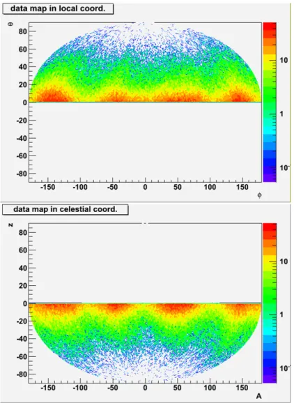
3.16.1 Observable sky . . . 56
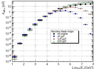
3.16.2 Effective area . . . 57
3.17 The current ANTARES detector . . . 57
4 Analysis of the 2007-2010 data 59 4.0.1 Definition of "run" . . . 61
4.0.2 DATA and DATA scrambled . . . 61
4.1 The coordinate convention system . . . 62
4.2 Data . . . 65
4.2.1 Configuration of the detector . . . 66
4.2.2 Types of runs . . . 67
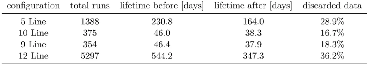
4.3 Data Quality selection of runs . . . 67
4.3.1 The detector lifetime of the data sample . . . 69
4.4 Construction of the detector simulation . . . 71
4.5 The background Monte Carlo . . . 72
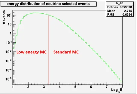
4.5.1 Standard and low energy Monte Carlo . . . 72
4.5.2 Monte Carlo and Data Quality selection . . . 73
4.6 The reconstruction algorithm . . . 74
4.6.1 The choice of the reconstruction algorithm . . . 77
4.7 The event selection . . . 79
4.7.1 Basic cuts and efficiency . . . 79
4.8 Weights policy for MC background events . . . 81
4.8.1 The standard formalism for weights . . . 81
4.8.2 How to use the weights . . . 83
Contents V
4.9.1 Angular resolution . . . 89
4.9.2 The effective area . . . 90
4.10 Monte Carlo simulation of ‹µ from Dark Matter . . . 90
4.10.1 The WIMPSIM package . . . 91
4.10.2 The annihilation spectra . . . 92
4.11 Weights policy for MC signal events . . . 93
4.11.1 The weight w2 in the v1r2p5 version of AntDST . . . 93
4.11.2 The signal weight convolution . . . 96
4.12 The selection of signal events . . . 97
4.12.1 Selection of ‹ candidates: the acceptance region . . . 97
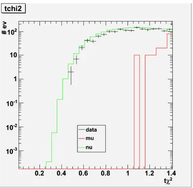
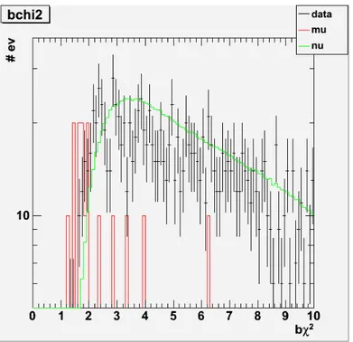
4.12.2 Selection of ‹ candidates: the cut t‰2 < b‰2 . . . 98
4.13 The binned analysis . . . 100
4.14 The statistical analysis of 2007-2010 data . . . 104
4.14.1 The Model Rejection Factor . . . 105
4.14.2 The cuts to optimize . . . 106
4.15 Final results and conclusions . . . 108
Conclusioni 113 A The Feldman and Cousins statistical approach 115 A.1 Bayesian interval construction . . . 115
A.2 Classical Neyman’s interval construction . . . 116
A.3 Poisson process with background and Feldman and Cousins ordering principle . . . 117
A.3.1 Our Feldman and Cousins construction of intervals . . . 118
B The Cross-Talk effect in ANTARES ARS 123 B.1 Structure and description of an ARS . . . 123
B.1.1 TVC . . . 125
B.1.2 AVC . . . 126
B.2 The cross-talk effect between the measures of time and charge . . . . 127
B.3 The study of the time evolution of the cross-talk parameters . . . 129
B.3.1 The first part of the analysis . . . 130
B.3.2 The second part of the analysis . . . 133
VII
Introduzione
Lo scopo di questa tesi è la ricerca di neutrini provenienti dall’annichilazione di materia oscura nel centro galattico.
Nella nostra ricerca usiamo i neutrini come portatori di informazioni astronomiche. Potrebbe suscitare curiosità il motivo che ci spinge ad usare i neutrini (pochi e difficili da rivelare) invece dei più abbondanti fotoni. Certo i fotoni sono abbondanti e facilmente rilevabili, ma se vogliamo studiare le regioni più dense e calde del cosmo, motori di molte sorgenti astrofisiche, queste risultano opache ai fotoni e quindi non indagabili direttamente. Inoltre i fotoni possono subire anche l’effetto della radiazione cosmica di fondo (CMB) producendo, nell’interazione, coppie elettrone-positrone. Anche i protoni, se decidiamo di usarli per fare astronomia, risentono dell’interazione con la CMB. Oltretutto i protoni, essendo particelle cariche, vengono deviati dalla presenza dei campi magnetici (per energie < 1019 eV) perdendo l’informazione della
sorgente originaria. I neutrini possono invece rivelarsi una buona scelta per condurre indagini astronomiche. Infatti essi sono debolmente interagenti, quindi penetrano le regioni opache ai fotoni; sono elettricamente neutri, non subiscono dunque l’influenza di campi magnetici; infine sono stabili e possono viaggiare per lunghe distanze inalterati. Come vedremo, essi costituiscono un valido oggetto d’indagine per la ricerca di annichilazione di particelle di materia oscura in oggetti astrofisici.
Negli ultimi decenni, numerose osservazioni di oggetti astrofisici di diverso tipo hanno portato all’ipotesi dell’esistenza di una forma di materia invisibile, perciò detta oscura, ma preponderante nel bilancio totale della materia presente nell’Universo (capitolo 1).
Le più note evidenze osservative della presenza di una forma di materia non bari-onica nell’Universo sono: la curva di velocità rotazionale nelle galassie a spirale, curva che rimane costante (vr≥ cost) anche a grandi distanze r dal centro delle galassie, contrariamente all’andamento aspettato (1/Ôr); l’esistenza stessa degli ammassi di galassie che, date le altissime velocità del gas intra ammasso (≥ O(1000 km/s)), dovrebbero invece disgregarsi; la ormai celebre analisi dello scontro del "bullet cluster" con un altro ammasso, in cui le buche di potenziale tracciano la materia visibile (stelle) e non il gas caldo visibile nell’X che dovrebbe rappresentare la parte maggiore della materia di un ammasso; ed ultimo, la presenza stessa di strutture cosmiche nel nostro Universo, inspiegabile senza l’ipotesi di una forma di materia nuova che, disaccoppiandosi prima della materia ordinaria dall’Universo primordiale, avvia la formazione di aloni di materia oscura in cui poi andranno a cadere le particelle della materia ordinaria (barionica) che formano le strutture che oggi vediamo intorno a noi nell’Universo.
VIII Introduzione non esiste nel modello standard alcuna particella che soddisfi le caratteristiche che dovrebbe avere tale forma di materia: elettricamente neutra, stabile e che interagisca solo per interazioni debole e gravitazionale. Per questo si ricorre a modelli che prevedano espansioni del modello standard delle particelle elementari.
Il modello usato più comunemente è quello della espansione supersimmetrica (SUSY) del modello standard (capitolo 2). In particolare nel modello supersimmetrico minimale (MSSM) le particelle di materia oscura vengono identificate con i neutralini più leggeri ‰. Queste particelle, che hanno le proprietà di particelle Majorana (quindi anti particelle di se stesse), vengono anche chiamate WIMP (Weak Interacting Massive Particles).
I WIMP dell’alone di materia oscura della galassia si accumulano nel centro incrementando la densità di materia oscura nel Centro Galattico; oppure possono essere attratti gravitazionalmente da oggetti massivi come le stelle (come il Sole) o i pianeti. In questi ultimi casi, per mezzo di successive collisioni elastiche, i WIMP vengono attratti nel centro di questi oggetti; qui si annichiliscono formando varie particelle secondarie (bosoni, quark, leptoni). La maggior parte di queste viene subito riassorbita, ma alcuni danno origine, decadendo, a neutrini che possono essere rivelati sulla Terra. Considerando i vari canali, la massa del neutrino risultante può andare da circa 1/3 a circa 1/2 della massa del WIMP. Considerando che i vari modeli supersimmetrici prevedono la massa del WIMP nell’intervallo 100 Gev ≠ 1 TeV , i neutrini risultanti hanno energie ben diverse da quelle tipiche dei neutrini solari (pochi MeV ) e possono essere rivelati qui, sulla Terra, per mezzo di telescopi per neutrini. Dati i piccoli flussi aspettati e la piccolissima sezione d’urto dei neutrini (‡‹ ¥ 10≠38· E[GeV ]) necessitiamo di grandi volumi instrumentati per la rivelazione. Solitamente si usa la tecnica di rivelazione di luce Cherenkov, quindi un’altra necessità è disporre di un grande mezzo che sia trasparente: acqua e ghiaccio sono mezzi ottimali.
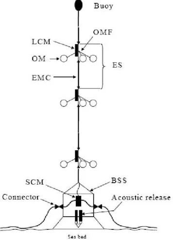
Nella nostra analisi utilizziamo i dati raccolti dall’esperimento ANTARES. ANTARES è un telescopio sottomarino per neutrini basato sulla tecnica Cherenkov (capitolo 3). Esso è composto da dodici stringhe, di 350 m di altezza, instrumentate con fotomoltiplicatori (PMT). Le stringhe sono ancorate al fondo marino a circa 2400 m di profondità al largo della costa mediterranea francese. I neutrini che interagiscono in corrente carica con la materia nei dintorni dell’apparato producono nell’interazione leptoni carichi che, attraversando il detector, possono essere rivelati per mezzo della luce Cherenkov che essi inducono. In questo modo è possibile ricostruirne la direzione di provenienza e l’energia. La rivelazione di neutrini muonici, che producono muoni nell’interazione con la materia, è l’obiettivo principale per cui è stato costruito l’apparato, anche se esso può rivelare anche gli altri sapori di neutrino.
Il problema principale è identificare gli eventi si segnale e distinguerli da quelli, molto più numerosi, di fondo. I tipi di fondo riscontrabili nell’esperimento ANTARES sono due: i muoni atmosferici ed i neutrini atmosferici prodotti nell’interazione dei raggi cosmici con l’atmosfera terrestre. Per minimizzare il fondo cerchiamo i cosid-detti eventi up-going cioè provenienti da sotto l’orizzonte del rivelatore (principal-mente dall’emisfero sud). In questo modo la Terra agisce come uno scudo che elimina il fondo di muoni atmosferici dal basso ma non quello dei neutrini atmosferici che, interagendo con la materia sul fondo dell’apparato, producono muoni che vengono
IX rivelati dal detector. Bisogna però considerare che i neutrini atmosferici di fondo sono distribuiti isotropicamente mentre gli eventuali neutrini di segnale provengono da una ben precisa direzione. Quindi osservare un eccesso statistico di eventi di neutrino in una data direzione può costituire una evidenza di segnale. Le tracce di eventi provenienti dall’alto (muoni e neutrini astrofisici) vengono scartate in sede di analisi dati considerando anche che ANTARES è ottimizzato per la rivelazione di eventi dal basso. In aggiunta alle tracce di fondo occorre considerare anche la bioluminescenza naturale marina e il decadimento del potassio presente nel mare. Questo rumore ottico è minimizzato considerevolmente con l’ausilio di sofisticati sistemi di trigger studiati per l’apparato.
In questa analisi usiamo i dati raccolti dall’esperimento ANTARES nel periodo di presa dati 2007-2010 (capitolo 4). Per scartare i dati acquisiti in periodi con un ambiente marino in cattive condizioni e per selezionare solo dati presi con un apparato attivo e perfettamente funzionante si stabiliscono dei criteri di qualità da applicare alla totalità dei dati considerati. Nell’intervallo di tempo suddetto, dopo i tagli di qualità, il tempo attivo di presa dati risulta pari a circa 588 giorni di osservazione.
Nell’analisi abbiamo esaminato il set di dati e le corrispondenti simulazioni Monte Carlo (MC) del fondo e del segnale. Le simulazioni MC ci aiutano a descrivere tutte le forme di fondo fisico (muoni e neutrini atmosferici) che contaminano la rivelazione del segnale (costituito da neutrini muonici provenienti dall’annichilazione di materia oscura nel Centro Galattico). Le simulazioni MC vengono anche usate per rappresentare la risposta del rivelatore agli eventi di segnale e di fondo. Sia gli eventi di fondo simulati col MC sia i dati grezzi vengono ricostruiti tramite un programma di ricostruzione di eventi chiamato BBFit.
Neutrini muonici da sorgenti puntiformi, o da annichilazione di WIMPs, sono segnali molto rari. Dunque, imponiamo dei tagli stringenti, su determinati parametri fisici, per selezionare un campione di dati arricchito in segnale. Quest’ultima è la parte più importante dell’analisi.
Per costruire una realistica simulazione MC di segnale da annichilazione di materia oscura nel Centro Galattico usiamo il pacchetto WIMPSIM. In particolare abbiamo scelto di porre dei limiti sulla sensibilità dell’apparato per tre diversi canali di annichilazione dei WIMP (‰‰ ≠æ b¯b, ·+·≠, W+W≠) e per dieci masse diverse
da 50 GeV a 1 T eV per un totale di 29 modelli differenti di materia oscura. La ricerca di neutrini da annichilazione di materia oscura nel Centro Galattico è una ricerca di sorgente puntiforme. Portiamo quindi avanti una ricerca detta "binned": cerchiamo eventi di segnale in coni angolari di apertura fissata centrati in
direzione del Centro Galattico.
Come abbiamo detto, l’unico modo di rivelare un segnale di neutrini dal Centro Galattico consiste nel riscontrare un eccesso statistico di eventi sopra il sottostante fondo. L’ultimo passaggio dell’analisi dei dati 2007-2010 corrisponde alla ottimiz-zazione del set dei due parametri rappresentanti la qualità della ricostruzione della traccia di muone e la semiapertura del cono angolare centrato nel Centro Galattico. Per calcolare la significatività statistica del risultato usiamo l’approccio di Feldman e Cousins (appendice A) applicando il metodo dell’MRF (Model Rejection Factor) per ogni modello di materia oscura preso in considerazione. Con i valori dei tagli ottimiz-zati possiamo alfine minimizzare l’MRF e valutare la sensibilità dell’esperimento
X Introduzione ANTARES alla rivelazione di flussi di neutrini provenienti dall’annichilazione di particelle di materia oscura nel Centro Galattico.
In appendice abbiamo descritto il lavoro di calibrazione svolto all’interno della collaborazione ANTARES (appendice B) parallelamente a quello di analisi di fisica. Questo lavoro concerne la calibrazione di circuiti, presenti in ogni PMT, che per-mettono di acquisire il segnale analogico dato dai fotoni Cherenkov e convertirlo in segnale digitale per poi spedirlo a terra per l’analisi. Questi circuiti, chiamati ARS, misurano anche la carica dei segnali ed i loro tempi d’arrivo sul fototubo. Gli ARS presentano un problema di "cross-talk" (diafonia) tra la parte del circuito che misura la carica e quella che misura il tempo. Lo scopo di questa nostra attività di calibrazione è cercare di studiare questo effetto e trovare una correzione universale, stabile nel tempo, da poter applicare a tutti i dati acquisiti dal rivelatore.
Ora descriviamo concisamente l’argomento di ciascun capitolo di cui si compone questa tesi.
Nel primo capitolo descriviamo in linea generale il modello standard dell’Universo. Partiamo dall’enunciazione del principio cosmologico e dalla constatazione dell’espansione dell’Universo (paragrafo 1.1). Descriviamo quindi la metrica che si usa per un universo omogeneo ed isotropo (paragrafo 1.2). Passiamo poi alla rassegna delle principali componenti in energia dell’Universo e alle equazioni che ne regolano l’espansione (paragrafo 1.3). Raccontiamo poi una storia sommaria della sua evoluzione dai tempi subito dopo l’istante iniziale ad oggi (paragrafo 1.4). Nella seconda parte del capitolo introduciamo le evidenze che permettono di ipotizzare la presenza di materia oscura come componente principale costituente la materia nell’Universo (paragrafo 1.5). Da ultimo introduciamo i WIMPs (paragrafo 1.6) e i metodi per una loro rivelazione (paragrafo 1.7).
Nel secondo capitolo introduciamo la teoria supersimmetrica di espansione del mod-ello standard delle particelle elementari (paragrafo 2.1). Trattiamo brevemente il modello minimale supersimmetrico (paragrafo 2.2) nel cui ambito è definita la particella supersimmetrica più leggere che viene identificata con il neutralino più leggero. Questa particella è quella più comunemente presa a modello per comporre la materia oscura (paragrafo 2.3).
Nel terzo capitolo descriviamo in dettaglio il telescopio per neutrini ANTARES. Per prima cosa spieghiamo il principio di rivelazione dei neutrini con l’apparato (paragrafo 3.1) e le diverse tipoogie di interazioni di neutrino visibili in ANTARES (paragrafo 3.2). Parliamo quindi brevemente dell’effetto Cherenkov (paragrafo 3.3) e della propagazione della luce in acqua (paragrafo 3.4), quindi schematizziamo la tecnica di ricostruzione delle tracce di eventi nell’apparato (paragrafo 3.5). Ci addentriamo poi nella descrizione del disegno del
rivela-tore (paragrafo 3.7), ne facciamo una panoramica generale (paragrafo 3.8) e passiamo in seguito a descrivere una stringa tipo (paragrafo 3.9). Nel seguito descriviamo la struttura e le caratteristiche dei fotomoltiplicatori (paragrafo 3.10) e l’elettronica di supporto (paragrafo 3.11). Segue la descrizione del sistema di "slow-control" dell’apparato (paragrafo 3.12), la calibrazione
(para-XI grafo 3.13), il sistema di posizionamento acustico delle stringhe (paragrafo 3.14) e l’analisi del rumore ottico di fondo dato dalla bioluminescenza marina e dal decadimento del potassio marino disciolto in acqua(paragrafo 3.15). Per concludere il capitolo mostriamo il cielo osservabile da ANTARES, l’area efficace dell’esperimento (paragrafo 3.16) ed il suo stato attuale (paragrafo 3.17).
Nel quarto capitolo definiamo il set di dati utilizzati (paragrafo 4.2) e la selezione di qualità applicata al set di dati per scartare quelli presi in periodi con un ambiente marino instabile (paragrafo 4.3). Ci occupiamo poi di descrivere come si costruisce una simulazione Monte Carlo dell’apparato (paragrafo 4.4). Dopo la definizione dei sistemi di coordinate usate per identificare una sorgente sulla sfera celeste (paragrafo 4.1), introduciamo il Monte Carlo che simula il fondo (paragrafi 4.5 e 4.8) e discutiamo in dettaglio l’algoritmo che ci permette di ricostruire le tracce di muoni rivelate dal detector (paragrafo 4.6). Quindi de-scriviamo la selezione di base degli eventi accettati (paragrafo 4.7) e mostriamo i grafici di confronto tra dati e Monte Carlo di fondo (paragrafo 4.9). Dopo il confronto tra i dati ed il MC di fondo passiamo alla costruzione del Monte Carlo di segnale che simula il segnale di neutrini aspettato dall’annichilazione di materia oscura nel Centro Galattico (paragrafi 4.10 e 4.11). Nell’ultima parte del capitolo trattiamo la selezione degli eventi di segnale (paragrafo 4.12), discutendone le ragioni e le finalità, quindi descriviamo l’analisi detta "binned" del set di dati (paragrafo 4.13), arrivando a definire la significatività statistica (secondo l’approccio di Feldman e Cousins) della nostra analisi (paragrafo 4.14) e mostrando i grafici della sensibilità di ANTARES a flussi di neutrini da annichilazione di WIMPs nel Centro Galattico (paragrafo 4.15).
Nell’appendice A è illustrato l’approccio statistico di Feldman e Cousins. Partendo dall’approccio classico di Neyman, passando per la statistica Bayesiana, si arriva a definire un nuovo metodo per la costruzione degli intervalli di confidenza per una misura sperimentale dato un certo livello di fondo.
Nell’appendice B descriviamo il lavoro di calibrazione dei circuiti ARS svolto all’interno della collaborazione ANTARES. Introduciamo i circuiti per la misura della carica e del tempo di arrivo dei segnali e la problematica dell’effetto di "cross-talk" tra questi due elementi. Quindi procediamo con la descrizione dello studio portato avanti per stabilire una correzione universale indipendente dal tempo per tutti i dati raccolti dall’esperimento.
1
Chapter 1
The standard model of
cosmology and Dark Matter
In this chapter [125,50,56] the standard cosmological model is described. This model is currently considered the most appropriate to explain almost all the astrophysics observations available. As the base of this model there is the cosmological principle. From this first assumption one can add, thanks to the use [116] of the general relativity and of the Einstein equations in particular, all the diverse components that form all together the so called CDM model.
After this brief description of the standard model of cosmology, that serves for contextualization, the dark matter scenario will be described. The different models and candidates for the role of dark matter particles will be shown.
1.1 Standard model of the Universe: first principles
In this section we will explain the cosmological principles, that are at the base of the standard model, the concept of redshift and the Hubble law, that describe the expansion of the Universe. With the Hubble law we can then evaluate in a simple way the age and the size of the Universe.
1.1.1 The cosmological principle
In the first years of the XX century the knowledge about the distribution, composition and metric of matter in the Universe was very poor. Friedmann was the first to find the solution of the Einstein equations for a homogeneous distribution of matter, but he never hypothesised the cosmological principle.
Thus, in the lack of observational data and with the aim of finding a simple model to describe our Universe, that could be used as a foundation for mathematical and geometrical theories, one has recourse, at the end of ’40 years, by Gamow [74, 17], to the formulation of the cosmological principle. This formulation has been revealed, thanks to the definition of new techniques that have brought to an incredible development of our knowledge of the Universe, correct.
2 1. The standard model of cosmology and Dark Matter
Theorem 1 (Cosmological principle) The Universe is homogeneous
and isotropic on large scales (Ø 100 Mpc).
It means that, in it, there not exist privileged positions or directions (following the Copernican principle). The concepts of homogeneity and isotropy appear to be strange to us in rapport to our perception of the Universe: stars, galaxies and other structures separates from each other by great empty spaces, thus a completely anisotropic and inhomogeneous scenario! This is the reason because, in the principle, one refers to the big scales1.
Thus, roughly above 100 Mpc, the Universe appear isotropic from our point of view in the space. But the isotropy in a given point in the space, combined with the cosmological principle, leads to the isotropy in any given point in the space, and the isotropy in any given point in the space implies the homogeneity of the Universe in any point.
1.1.2 The Universe is expanding
Let we take the spectrum of a galaxy and let us examine an absorption line of this spectrum. In a laboratory frame on Earth this line has a wavelength ⁄e, while the wavelength we observe, for the same line, in another galaxy is generally different and equal to ⁄o.
Now we define a quantity that has an enormous importance: the redshift (z), defined by:
z = ⁄o≠ ⁄e
⁄e . (1.1)
We need to specify that some galaxies show negative values of z, thus they undergo a blue-shift induced by their own motion, but almost all the galaxies show a red-shift of the spectral lines.
The Hubble law
In 1929 Hubble measured [87] redshift and distances of a sample of galaxies reporting his results in a redshift-distances diagram.
He, hence, found the relation that has his name:
v= cz = H0d. (1.2)
This is the Hubble law. More distant are the galaxies, more they are moving away from us. This regression is induced by their radial velocity v. In the formula 1.2 appears the Hubble constant H0. It has a measured value equal to H0 =
(71.9 ± 2.6) km/s/Mpc [71, 58].
The meaning of this law is that the galaxies move away from us and from each other linearly with the distance.
1.2 The metric of the Universe 3
The age of the Universe
Is interesting to note that, if today the galaxies are moving away from each other, there have been one moment in which they were very closed each other, all in the same point. In the absence of external forces the velocities of two galaxies, with a distance d between them, will be constants.
Thus, at a given time we have:
t0 = dv = Hd 0d = H
≠1
0 , (1.3)
where we made use of the Hubble law 1.2. The t0time is called Hubble time. With
the reported above value of the Hubble constant it is equal to t0= (13.69±0.13) Gyr
[95].
Thus, roughly 14 billions of years ago all the galaxies were forced in a point in the space. Consequently the Hubble time is a raw estimation of the age of the Universe. This value is also confirmed by the age of the most ancient stars that is compatible with it.
This is a simple scheme of the Big bang model, according to this theory, the Universe is evolved from a very little, dense and hot initial volume to the current enormous, rarefied and cold volume.
The size of the Universe
As we did for the age of the universe, the Hubble law 1.2 can be also useful to define a scale of interest in cosmology. This scale corresponds to the maximum distance that a photon can cover from the Hubble time until today.
This distance is called Hubble distance:
dH(t0) = c
H0 = (4300 ± 400) Mpc. (1.4)
It can be considered like a raw estimation of the maximum size of the Universe.
1.2 The metric of the Universe
Now we try to build models of the Universe that respect the cosmological principle and based on the general relativity. Since the general relativity [130] is also a geometrical theory let we now examine the geometrical properties of an homogeneous and isotropic space.
Let us assign to each point in the space the three space coordinates, constant in time, x– with (– = 1, 2, 3) and one time coordinate (– = 0): the so called proper
time (measured by a clock in motion with the point). The coordinates x– are called the co-moving coordinates.
If the matter distribution is uniform, then the space is homogeneous and isotropic and the proper time become the time measured by an observer that sees the Universe uniformly expanding around it, such as the three-dimensional space metric dl2
between space points is identical in any time, place and direction to respect the cosmological principle.
4 1. The standard model of cosmology and Dark Matter Thus, the expression for the metric, following the synchronous gauge, is ds2=
(cdt)2≠ dl2. Taken into account these geometrical considerations (for a complete
treatment see [142]), the metric that describes, among all the possible choices, in the better way a Universe characterised by the cosmological principle is the
Friedmann-Robertson-Walker metric (FRW), that has the form: ds2= (cdt)2≠ a(t)2 C dr2 1 ≠ Kr2 + r2(d◊2+ sin2◊d„2) D . (1.5)
where (r, ◊, „) are the polar coordinates in the co-moving reference system (if the Universe’s expansion is perfectly homogeneous and isotropic, then the co-moving coordinates of any point in space remains constants in time), t is the proper time,
K is the curvature constant: it can assume the values 1,0 or -1 if the Universe has a
closed, flat or open geometry respectively [121].
It is important to note besides the introduction of a new time dependent function:
a(t) called the scale factor. It has the dimensions of a length and serves to describe
the expansion or the eventual contraction of the Universe, and it is normalised in order to have today a value a(t0) = 1. This means that a galaxy have, in its own
co-moving reference system, coordinates that do not vary with time, the thing that vary with the time is the metric itself.
1.3 The basis of the theory of the Universe
To derive the equations ruling in the Universe we have to start from the expression of the Einstein equation [69]:
Gµ‹ = Rµ‹≠ 1
2gµ‹R= 8fiGTµ‹, (1.6)
where we have set c = 12. G
µ‹ is the Einstein tensor, Rµ‹ = R‡µ‡‹ is the Ricci tensor (where R‡
µ‡‹ is the Riemann tensor that tells us if the space is flat or curve), gµ‹ is the metric tensor and Tµ‹ is the energy-momentum tensor, that describes the distribution of matter and energy in the Universe. R = gµ‹R
µ‹ is the so called scalar curvature.
The left side of the equation describes the geometry of the space-time, while the right side of the equation3 accounts for the energy contained in it. This is the main
aim of the Einstein equation: to bond the matter (and energy) to the metric of the space-time.
First we define the Hubble parameter, that is an estimation of the expansion rate of the Universe. It tells us how much the scale factor varies with time:
H(t) = da/dt a(t) =
˙a(t)
a(t). (1.7)
Following this notation the Hubble constant represents only the particular case
H(t0) = H0. The Hubble law 1.2 can be rewrote in this way: v = H(t)d. This is
2From now on we will always consider c = 1.
1.3 The basis of the theory of the Universe 5 the only velocity field compatible with the isotropy and homogeneity stated in the cosmological principle.
1.3.1 The ruling equations of the Universe
From the Einstein equation we can derive [56] the equation that governs the expansion of the Universe. This is the Friedmann equation:
H(t)2= 3˙a a 42 = 8fiG3 fl≠ K a2, (1.8)
where with fl all the kind of energy densities of the components of the Universe (matter, radiation and dark energy) are taken into account. K is the curvature
constant just explained above.
The Friedman equation alone can not specify the behaviour of the scale factor in time, because is an equation with two unknown variables (a(t) and fl(t)). Thus, we use the energy conservation law ˆTµ
‹/ˆxµ= 0.
Considering an expanding, homogeneous and isotropic Universe we can derive, from the continuity and Euler equations that govern the evolution of the density fl and of the pressure P respectively, the so called fluid equation:
ˆfl ˆt + 3
˙a
a(fl + P ) = 0. (1.9)
Combining the Friedmann equation 1.8 with the fluid equation 1.9, with some passages we arrive to the second equation of Friedmann, also called acceleration
equation:
¨a
a = ≠
4fiG
3 (fl + 3P ). (1.10)
From this equation is clearly visible that, if the energy density fl is positive, then we will have a negative acceleration, that is a deceleration of the Universe.
Now we have three equations with three unknown variables: a(t), fl(t) and P (t). However the last equation 1.10 it is not independent from the others two, so we need a further equation.
The last equation we need is a state equation, of the type P = P (fl), that bonds together the pressure with the energy density of the components of the Universe.
For any components of cosmological interest the equation of state can be written in the simple form:
P =ÿ
i
wifli, (1.11)
where w is a dimensionless constant with values that differ with the type of com-ponents i considered. Our set of equations (1.8, 1.9, 1.10 and 1.11) describing the Universe is now complete.
6 1. The standard model of cosmology and Dark Matter
1.3.2 The components of the Universe
In this section we take in consideration the principal components of the Universe: radiation, matter and dark energy. Combining the fluid equation 1.9, that holds for each component separately, with the equation of state 1.11 we obtain the evolution of the energy density for each component:
flw(a) = flw,0a≠3(1+w). (1.12)
With this equation we can evaluate the evolution of the energy density as a function of the scale factor and of the redshift.
From the different behaviour of the energy density fli of the diverse components as a function of the scale factor it is possible to see that the Universe undergo three different regimes in which was dominated by only one component each time. First there was the radiation domination, then the matter domination and last the dark energy domination.
Radiation
In the first part of its life the Universe was dominated by the radiation component. A not degenerate fluid of relativistic particles in thermal equilibrium has an equation of state parameter equal to w = 1/3.
Thus, form the state equation and the density evolution equation 1.24, using the relation that bonds redshift and scale factor ( 1
a(t) = 1 + z), we can derive the trend of the radiation energy density as a function of the scale factor and of the redshift, and from the Friedmann equation we can derive the evolution of the scale factor with the time and the relative Hubble parameter:
flr= fl0,ra(t)≠4= fl0,r(1 + z)4 a(t) = 3t t0 41/2 (1.13) H(t) = 2t1 Matter
After the radiation the matter component dominated the Universe. For the matter, considered as a non relativistic ideal gas with negligible pressure, w = 0.
This leads to:
flm= fl0,ma(t)≠3= fl0,m(1 + z)3 a(t) = 3t t0 42/3 (1.14) H(t) = 3t2
1.3 The basis of the theory of the Universe 7
Dark energy
Recently the Universe has been started to be dominated by the dark energy compo-nent, which physical meaning is not yet understood [127]. Supposing the dark energy being fully described by the so called cosmological constant (first introduced and then rejected by Einstein) that have a w = ≠1, we obtain:
fl = constant
a(t) = exp[H0(t ≠ t0)] (1.15)
H(t) = H0
From the above reported behaviour of the scale factor, energy density and Hubble parameters we can derive the moments in which there were the passages of the domination phases between the different components.
As we have seen, the radiation energy density decreases more quickly than the matter one. The passage epoch is called radiation-matter equivalence. Equating the densities we obtain:
arm= 0,r
0,m ƒ 2.8 ◊ 10 ≠4
zrm= a≠1rmƒ 3600 (1.16)
The second moment of equivalence, this time between matter and dark energy, happens at: am = 3 Û 0,m 0, ƒ 0.75 zm ƒ 0.33 (1.17)
1.3.3 The cosmological parameters
For a flat Universe, a critical density can be defined as:
flcr= 8fiG3 H02. (1.18)
If the Universe has a critical density bigger than this value it will have a positive curvature (K = 1), otherwise it will have a negative curvature (K = ≠1). Currently the critical density has a value equal to flcr= (9.2 ± 1.8) ◊ 1029 g/cm3 [77].
It is useful to introduce some new variables. Let we define the dimensionless density parameters:
i= fli
flcr
. (1.19)
With (t) > 1(K = 1) we have a closed Universe, with (t) < 1(K = ≠1) we have an open Universe for (t) = 0 we have a flat Universe. Remember that a Universe ruled by the Friedmann equation cannot change its curvature’s sign.
With this new formalism the Friedmann equation, at the time t0, becomes:
8 1. The standard model of cosmology and Dark Matter In this formula is evident the dependence of the curvature of the Universe from its total energy density. Since we know that our Universe is flat ( K = 0), thus described by an euclidean geometry, the Friedman equation can be rewrote in the following way taking into account all the contributes to the today Universe’s energy density:
1 = 0,tot= 0r+ 0m+ 0 . (1.21)
Then to describe in the correct way the behaviour of our Universe it is necessary to know the values of the main cosmological parameters ( r0: radiation, m0: matter,
0 : dark energy) present in the above equation 1.21.
A lot or recent measures [34, 95,25] posed constraints over these parameters. • r= “(1 + 0.2271Nef) – Nef ¥ 3.04 – “ ¥ 4.76 ◊ 10≠5 • m¥ 0.258 ± 0.030 – bh2¥ 0.02273 ± 0.00062 – ch2¥ 0.1099 ± 0.0062 • ¥ 0.742 ± 0.030
Thus, as can be also seen from the parameters characterizing the dark energy component , the Universe expansion is accelerating exponentially. The acceleration is also confirmed by the deceleration parameter q04.
For a Universe containing the three major components described in the paragraph 1.3.2, this parameter can be expressed in the following way:
q0= ≠ 3¨aa ˙a2 4 t=t0 = 0,r+ 12 0,m≠ 0, (1.22)
Thus a positive value of q0 corresponds to a negative acceleration and vice-versa.
Recent measures of this parameter gave the value q0 ƒ ≠0.55: an accelerating
Universe.
1.4 Brief summary of the history of the Universe
In this section we will briefly describe [115] the history of the Universe with the diverse ages and their characterizing events.
The observed expansion of the Universe [135,102], as we have seen in the section 1.3 and in the paragraph 1.1.2, is a natural result of any homogeneous and isotropic cosmological model based on general relativity and ruled by the Friedmann equations. However the Hubble expansion (1931) [87], by itself, does not provide sufficient evidence for what we generally call the Big-Bang model of the Universe. The 4This parameter has been called in this way because when it was first introduced (half of the
XX century), scientists thought, because of the lack of observational data, that the Universe was decelerating.
1.4 Brief summary of the history of the Universe 9
Figure 1.1. Probability contours for , m in sky blue. Regions representing specific cosmological sceneries are illustrated: models of closed, flat or open Universe and the possible future evolutions. Data of the Supernova cosmology project. The region of maximum probability is consistent with an accelerated and dark energy dominated Universe [124].
formulation of the Big-Bang model began, as we said, in the 40s years by Gamow and his collaborators. They proposed that the early Universe was very hot and dense (enough to allow the nucleosynthesis (BBN) of the Hydrogen) and expanded and cooled step by step to its present state [74, 17]. Alpher predicted (1948) that, as a consequence of this model, a relic background radiation had to be survived [18,19] with a temperature of roughly 3 K. This radiation was then (1965) observed by Penzias and Wilson: it is the Cosmic Microwave Background (CMB) [117]. This confirmed the Big-Bang theory as the prime candidate to describe the Universe. But there were some problems with the initial conditions of the model. These were solved (1981) with the inflationary solution proposed by Guth [81].
Inflation
Proposed by Guth to solve the horizon, flatness and monopoles problems (see [50] for details) the Inflation mechanism describes the behaviour of the Universe in the first moments of its life. It does not modify the sequent Big-Bang model of structure formation and evolution of the Universe. The Inflation states that from an age of the Universe equal to ti = 10≠36 suntil the age te= 10≠32s, the Universe underwent
10 1. The standard model of cosmology and Dark Matter an accelerated expansion of the scale factor. Thus, in the short duration of only 10≠34 s the Universe expanded by the enormous factor 1030!
The early times
At the beginning, in the first decimal of seconds, the temperature, the density and the pressure were so high that the matter, in the way we know it today, could not existed. The early Universe was a plasma made of relativistic elementary particles (quarks, neutrinos etc.) and photons. For the long time of the primordial life of the Universe, the interactions rate between these elements proceed with such a big rapidity that all the particles were in thermal equilibrium and different species shared the same temperature. Thus, in the absence of external energy exchange, the expansion was adiabatic.
Due to the expansion of the Universe, certain rates may be too slow to either establish or maintain equilibrium. Quantitatively, for each particle type i, as a minimal condition for equilibrium, one requires that some rate iinvolving that type must be larger than the expansion rate (given by the Hubble parameter at that time) of the Universe H: i> H. Recalling (paragraph 1.1.2) that the age of the Universe is determined by the equation 1.3, this condition is equivalent to requiring that, on average, at least one interaction has occurred over the lifetime of the Universe.
Good examples of particles that were before in the thermal equilibrium and, when their rates became smaller than the expansion rate, decoupled proceeding autonomously with the evolution are the neutrinos and the photons. Neutrinos went out of the equilibrium before of the photons (this happened when the Universe was 1 s old at a temperature of 9 ◊ 109 K), then their background temperature is now
smaller than that of photons: T‹ ƒ 1.9 K [143]. The neutrino density parameter is ‹h2= 5 ◊ 10≠4, so the neutrino contribution to the matter budget is negligible.
The baryogenesis
When the Universe was very hot and dense and the temperature was of the order of
M eV /kB5, there were no neutral atoms or bonded nuclei. The radiation domination in such a hot ambient assured that each atom or nucleus produced have been immediately destroyed by an high energy photon.
When the temperature of the Universe become of the order of 1 MeV , the pri-mordial cosmic plasma is composed of: relativistic particles in equilibrium (electrons and protons strongly coupled by the Compton scattering e+e≠≠æ ““), relativistic
decoupled particles (neutrinos) and non relativistic particles (baryons).
The initial process of baryogenesis had an asymmetry in the numbers of baryons and anti-baryons of the order of 10≠10 constant along all the expansion. Under
1 MeV all the anti-baryons were annihilated, thus the baryon to photon ratio is
÷b= nb/n“ = 5.5 ◊ 10≠10( bh2/0.020). 5The Boltzmann constant has the value k
1.4 Brief summary of the history of the Universe 11
The nucleosynthesis
When the cooling of the Universe arrive at a temperature lower than that of the bound energy of the nuclei, the first light elements start to form [108].
The nuclear processes lead primarily to Helium 4He, with a primordial mass
fraction of about 25%. Lesser amounts of the other light elements are produced: about 10≠5 of Deuterium D and Helium 3He and about 10≠10 of Lithium 7Li by
number relative to the Hydrogen H. The abundances of the light elements (see figure 1.2) depend almost only from the baryon-photon ratio we have shown in the previous sub-paragraph. The nucleosynthesis happened from 1 s to roughly 200 s (T ƒ 7 ◊ 108 K) of the life of the Universe.
The few number of neutrons with respect to protons show the inefficiency of the BBN. Still today the 75% of the baryon matter is composed by free protons and almost the 24% of baryon objects, like stars and gas clouds, are composed by Helium.
Figure 1.2. Constraint on the baryon density from Big Bang Nucleosynthesis. Predictions are shown for four light elements: 4He, D,3Heand7Li. Spanning a range of ten order of magnitude. The solid vertical band is fixed by measurements of primordial Deuterium. The boxes are the observations; there is an upper limit on the primordial abundance of 3He[56].
Recombination
It is the time in which the baryon component of the Universe passes from a totally ionised situation to a neutral one. It can be defined as the time in which the ions
12 1. The standard model of cosmology and Dark Matter numerical density is equal to the neutral atoms numerical density. The ionization rate can be expressed by the ionization fraction X = ne/nb.
The recombination took place for X = 1/2 when the temperature of the Universe was of the order of Trec= 3740 K. This happened at a redshift of zrec= 1370 that is when the Universe was 240000 age old; it last roughly for 70000 years: it is not an instantaneous process.
Decoupling
It is the time at which the scattering rate of the photons over the electrons become smaller than the Hubble parameter, that represents the expansion rate of the Universe. The decoupling happen when (zdec) = H(zdec). With zdec ¥ 1100, when the Universe was 350000 year old and the temperature was of the order of
Tdec = 3000 K.
Last scattering epoch (CMB)
It is the time at which a photon of the thermal bath undergo its last scattering from the free electron of the strongly coupled baryon-photon fluid. Thus each observer in the Universe has a last surface scattering around him. After this moment the photons has been free to travel in the space. This last scattering happened at
zls ¥ zdec= 1100. It is important to note that the last three epoch described here: recombination, decoupling and last scattering happened after the radiation-matter equivalence time, thus in the matter dominated Universe. This implies also that these results are dependent from the cosmological model assumed.
The relic of the last scattered photons were first observed by Penzias and Wilson in 1965. They found an isotropic background of microwave radiation. The temperature, with a perfect Planck law of black body spectrum, of this Cosmic
Microwave Background (CMB) was measured by the COBE satellite in 1992: TCM B = (2.725 ± 0.001) K [105].
Another observable quantity inherent in the CMB is the variation in temperature from one part of the microwave sky to another one [131,149]. These anisotropies are of the order ofÈ T/T Í2 ¥ 10≠5and were first observed by COBE and then better
investigated by WMAP [86] and are one of the main aim of the Planck experiment (see figure 1.3).
The structures formation
Before the decoupling age the strongly coupling of the baryon-photon fluid tend to destroy all the possible fluctuations in the density of the plasma. After the last scattering epoch we have two separated gases: baryons and photons. From now on the baryon component is free to collapse under its own gravity falling in the potential wells created by the dark matter (DM) component (see section 1.5). This collapse permit to form, in the time passed from the last scattering until today, all the cosmic structures we can see: from the giants clusters of galaxies till the smaller asteroid.
1.5 Dark Matter 13
Figure 1.3. CMB temperature anisotropies maps. In the left upper plot the sky map observed by COBE while in the right upper plot the sky map resolution of Planck. In the bottom portions of sky maps resolution are showed for WMAP (2 and 8 years) and Planck (1 year prediction).
1.5 Dark Matter
The matter density parameter m has a great importance, although it no more represents the dominant component in the Universe. With this parameter we can know the composition of matter in the Universe: how much matter in the Universe is under the form of stars, gas etc.?
Currently the value measured for the matter density parameter, as we seen in the paragraph 1.3.3, is 0,m ƒ 0.3. Now we try to evaluate the different types
of ordinary baryon matter parameters to see in which amount they contribute to the total density matter parameter. The stars represent only the 0.5% of the total matter in the Universe: ú,0ƒ 0.004 [125] (estimated through the data derived from the star formation theory).
Also galaxies and galaxy clusters contains baryon matter under the form of hot gas [16], with temperature of the order of 106 K. They are not in the visible part
of the light spectrum but in the X part [23, 101]. All these contributes form the baryon matter6. From the BBN arise some strict constraints:
0,b ƒ 0.0267 [86].
The baryon matter parameter is too small to account for all the matter considered in the total matter density parameter, then the majority of this matter has a non baryon nature: DM ƒ 0.21. It is not visible but it is necessary to explain a lot of phenomena that would not be existent. This is the reason why it is called Dark
Matter.
14 1. The standard model of cosmology and Dark Matter
Figure 1.4. The pie scheme represents the divisions of the energy density in the Universe. As can be seen the dark matter represents the biggest part of the matter component of the Universe.
1.5.1 Dark matter properties and types
Candidates for non baryonic dark matter must satisfy several conditions: • they must be stable on cosmological time scales;
• they must interact weakly with electromagnetic radiation; • they must have the correct relic density.
Since the Universe is indeed dominated by non baryonic matter (see figure 1.4), it is obviously important to figure out the present density of various types of candidate particle expected to be produced in the early stages of the Big Bang. These relics are held in thermal equilibrium with the other components of the thermal bath of the Universe until they decouple. These relic candidates are divided into two classes:
Hot Dark Matter (HDM) and Cold Dark Matter (CDM). The former are relativistic
when they decoupled, the latter are non relativistic a the time of the decoupling [50].
Hot Dark Matter
Examples of this type of relics are the neutrinos. However, a lot of different measures (CMB, SN and galaxy survey) show that the relic of cosmic neutrino background is too small to account for all the non baryonic dark matter component of the Universe. As we saw in the section 1.4 ‹ < 0.048 at 95% C.L. [86, 58] that pose an upper limit on the neutrino mass equal to m‹ < 0.68 eV at 95% C.L., limits that are in agreement with those obtained in laboratory: m‹ < 2 eV [111]. But, over all these reasons, there is the fact that, if the dark matter was composed of relativistic particles, no one of the cosmic structures we observe today would be formed in the structures formation process [137].
Cold Dark Matter
Possible cold (non baryonic) dark matter candidates could be represented by the axions or the primordial black holes etc. The primordial black holes have been postulated in some strange cosmological models [93] and they must be formed before
1.5 Dark Matter 15 the BBN. Instead the axions [132] have been introduced to solve the strong CP problem of QCD; they naturally occur in super-string theories.
Then, the most diffuse and tested scenario is the Weak Interacting Massive Particle (WIMP) that will be described in the following section 1.6.
1.5.2 Observational evidences
In this paragraph we will describe some methods that are used to evidence the presence of dark matter in our Universe; we will see that dark matter is the dominant component among those that form the total matter distribution.
Rotational velocity of galaxies and the galactic halo
The classic approach to identify the presence of dark matter is the measure of the rotational velocity of stars in spiral galaxies. Consider a star in motion on a stable Keplerian orbit of radius r, which velocity is v, around the galactic centre. The star feels an acceleration given by ˙v = v2/r directed toward the centre of the galaxy and
originated by the gravitational attraction of all the matter M(r) contained in the sphere of radius r: ˙v = GM(r)/r2.
Equating the two expressions we obtain the relation between velocity and mass:
v=
Û
GM(r)
r . (1.23)
If the only matter is the luminous matter, one expect that the velocity would decrease, for large values or the radius, as v(r) Ã 1/Ôr. However, following [57,100], what one observe is that the velocity remains constant also until big values of r as can be seen in the figure 1.5.
In our own galaxy, for the solar orbit radius r ƒ 8.4 kpc, the velocity is v ƒ 220 km/s with little change out to the largest observable radius. Then it is usually assumed that the rotational velocity of the Sun corresponds to vŒ.
Figure 1.5. Observed rotational curve of the galaxy NGC 3198 (data points) compared to the prediction based considering only luminous matter (dashed line) [144].
16 1. The standard model of cosmology and Dark Matter This implies the existence of a dark halo. For a spherical matter distribution
dM(r) = 4fir2fl(r)dr we can obtain the density distribution of the halo using the
concept of v(Œ) expressed above:
fl(r) Ã v
2 Œ
r2 (1.24)
The local dark matter halo density in the Sun’s position has been estimated to be fl0ƒ 0.3 GeV/cm3 [111,91]. At some point, fl will have to fall off faster to keep the total mass of the galaxy finite, but we do not know at what radius it happens. Since the formula 1.24 is singular for r = 0, there is uncertainty on the Galactic Centre position. This uncertainty is solved parametrizing the radial dark matter density profile distribution. One famous parametrization is the Navarro Frank and
White (NFW) profile [112] (see paragraph 1.5.3).
Clusters of galaxies and weak lensing
Another way to identify the presence of dark matter is to look at its gravitational influence on visible matter: for example from the observations of clusters of galaxies [38] one can estimate the luminous mass and compared it to the predicted virial mass. Zwicky was the first to perform this calculus for the COMA cluster. Starting from the virial theorem, that bounds the kinetic energy of the cluster T = mÈvÍ2/2 with
its gravitational potential energy U = Gm2/2r in statical equilibrium: 2T + U = 0,
he estimated the virial mass of the COMA cluster: M Ã rÈvÍ2/G. Measuring the
velocity dispersion of the galaxies in the COMA cluster he noticed that there was a bigger amount of matter with respect to the one calculated only considering the luminous matter.
Figure 1.6. Shown above in the top panel is a color image from the merging bullet cluster 1E0657-558. The white bar indicate 200 kpc at the distance of the cluster. In the bottom panel is a Chandra image of the cluster. Shown in green contours in both panels are the weak lensing reconstruction. The white contours show the errors on the positions of the peaks and correspond to 68.3%, 95.5%, and 99.7% confidence levels. The blue crosses show the location of the centres used to measure the masses of the plasma clouds [49]. Measurements of the X-ray temperature of the hot gas in the cluster, which correlates with the gravitational potential felt by the gas, together with the study of weak gravitational lensing of background galaxies on the cluster can evidence the presence of dark matter [57].
1.5 Dark Matter 17 A particular example of the described method involves the Bullet cluster which recently (on cosmological time scales) passed trough another cluster. As a result, the hot gas forming most of the cluster’s baryonic mass was shocked and decelerated, whereas the galaxies in the clusters proceeded on their trajectories. Gravitational lensing shows that the potential wells trace the visible matter distribution and not the hot thermal gas distribution that is supposed to be the big part of the matter in the absence of dark matter (see figure 1.6). This is a direct empirical proof of the existence of dark matter [49].
1.5.3 The Galactic Centre
The presence of a dark halo in the galaxy is almost sure (according to the observable evidences, some of them shown above), the problem arise when considering the dark matter profile in the inner region of the galaxy.
The usual parametrisation for a dark matter halo density is given by:
fl(r) = ! fl0 r R "“#1 +!r R "–$—≠“– , (1.25) where r is the galacto-centric coordinate coordinate, R is a characteristic length (in the case of our galaxy is the galactic halo radius, roughly equal to 20 kpc [77]) and –, —, “ are free parameters. fl0 is the just defined galactic halo density
(¥ 0.3 GeV cm≠3).
There is consensus, at present, about the shape of the profile in the outer parts of halos, but not in the innermost regions, due to loss of numerical resolution in N body simulations and to the poor resolution in observation of rotation curves of outer galaxies [33].
Navarro, Frank and White found [112], with N-body simulations, that the profile could be well approximated at small radii with a power-law fl(r) = r“.
Observations of the velocity dispersion of high proper motion stars suggest the existence of a Super Massive Black Hole (SMBH) lying at the centre of our galaxy, with a mass MSMBH¥ 3.6 ◊ 106 M§, and accreting dark matter producing the so
called spikes [79].
The existence of such spikes would produce a dramatic enhancement of the annihilation radiation from the galactic center and consequently a large uncertainties that are associated with predictions of annihilation fluxes.
Furthermore, the scattering of dark matter particles by stars in the dense stellar cusp observed around the SMBH could substantially lowering the dark matter density near the Galactic center over 1010 yrs, due both to kinetic heating, and to capture
of dark matter particles by the SMBH [32].
In the region that contains also the GC (in an error circle of 0°.2 radius) the EGRET satellite observed (around 1 GeV ) an excess of gamma-ray radiation with respect to the expected emission of gamma-ray due to the interaction of primary cosmic ray with the interstellar medium (via p + X ≠æ fi0, He + X ≠æ fi0, where
X is an interstellar atom) [106].
Recently with the data of the Fermi satellite [1] (which has, with the LAT experiment, among one of its aim the indirect search for dark matter in the galactic
18 1. The standard model of cosmology and Dark Matter halo [68]) has been observed an excess of gamma-ray emission (at ¥ 130 GeV ) in the direction of the central region of the galaxy. Several hypothesis has been done to interpret this excess. Currently there are no evidences that it can be due to dark matter annihilation. For discussion and more details, among the big numbers of published articles, see [138, 146,48].
1.6 The WIMP scenario
Among the candidates for non baryonic dark matter (axions, primordial black holes etc.), that satisfied the three conditions reported in paragraph 1.5.1, the most diffused scenario is that of a dark matter made of the Weak Interacting Massive Particles (WIMPs).
The WIMP particles, indicated with ‰, have a mass ranging from 10 GeV up to few T eV , and with weak strength cross-sections. In the early Universe the WIMPs are in thermal and chemical equilibrium with the primordial plasma. In this scenario, their density would become exponentially suppressed when the Universe reached a temperature T < m‰. The WIMPs therefore freeze out of the thermal equilibrium once the rate of reactions, that change standard model particles into WIMPs and vice-versa, becomes smaller than the Hubble expansion rate of the Universe. After the freeze out, the WIMPs relic abundance remains constant accounting for the component of dark matter [57].
1.6.1 The WIMPs relic
The evolution of the number density of a generic species ‰ in the Universe, is described (following [50, 137,100]) by the Boltzmann equation:
dn‰ dt + 3 ˙a an‰= ≠ȇA· vÍn 2 ‰+ Â, (1.26)
where the term ˙a
a = H is the Hubble rate that takes into account the expansion of the Universe, ȇA· vÍn2‰is the rate of collisional annihilation (‡A is the cross-section for annihilation reactions, and v is the mean particle velocity);  denotes the rate of creation of particle pairs. If the creation and annihilation processes are negligible, one has the expected solution: n‰eq à a≠3. This solution also holds if the creation and annihilation terms are non zero, but equal to each other, i.e. if the system is in (thermal) equilibrium:  = ȇA· vÍn2‰eq.
Thus, the equation 1.26 can be written in the form:
dn‰
dt + 3Hn‰= ≠ȇA· vÍ(n
2
‰≠ n2‰eq). (1.27)
The equilibrium abundance is maintained by annihilation with its antiparticle ¯‰ into lighter particles l (‰¯‰ ≠æ l¯l) and vice versa (l¯l ≠æ ‰¯‰). In our case, the WIMP ‰ is a Majorana particle (‰ = ¯‰) [51].
The equilibrium density of WIMPs in the primordial plasma at temperature T and for a non relativistic specie is given, following the Boltzmann distribution, by:
n‰eq =
g
(2fi)3
⁄
![Figure 3.7. The angular distribution of light scattering in the deep Mediterranean Sea for (400 Æ ⁄ Æ 500) nm [ 109].](https://thumb-eu.123doks.com/thumbv2/123dokorg/5494235.62986/55.892.258.581.215.576/figure-angular-distribution-light-scattering-deep-mediterranean-sea.webp)