Thermodynamics of water and biosystems

(1)

Dipartimento di Scienze Matematiche e Informatiche, Scienze Fisiche e Scienze della Terra

D

OTTORATO DI

R

ICERCA IN

F

ISICA XXX Ciclo

T

HERMODYNAMICS OF

W

ATER AND

B

IOSYSTEMS

Dottorando: Sebastiano VASI

Tutore: Prof. Francesco MALLAMACE

Coordinatore: Prof. Lorenzo TORRISI

(2)

“All things are from water and all things are resolved into water.”

(3)

Riassunto

Il presente lavoro di tesi è incentrato sullo studio termodinamico dell’interazione dell’acqua con alcuni biosistemi, illustrando come l’acqua rivesta un ruolo importante nel "guidare" le proprietà di tali sistemi. In particolare, gli esperimenti sono stati condotti utilizzando la tecnica della Risonanza Magnetica Nucleare, passando dal metanolo, la più semplice molecola anfifilica, ad un sistema più complesso come il lisozima, una proteina enzimat-ica dotata di attività battericida.

Le misure di Risonanza Magnetica Nucleare sono state eseguite con uno spettrometro Avance della Bruker operante a 700 MHz ed utilizzando diverse tecniche e sequenze, tra cui il "Pulsed Field Gradient Stimulated Echo" e la "High-Resolution Magic Angle Spin-ning". La strumentazione utilizzata è localizzata nel Laboratorio di Fisica dei Sistemi Complessi gestito dal Prof. F. Mallamace, presso il "Dipartimento di Scienze Matem-atiche e InformMatem-atiche, Scienze Fisiche e Scienze della Terra" (MIFT) dell’Università di Messina.

Sono stati oggetto di studio molte grandezze dinamiche e termodinamiche dei sis-temi investigati, tra cui la diffusione, misure ottenute mediante l’utilizzo di gradienti di campo magnetico che permettono di effettuare una codifica spaziale delle frequenze di precessione degli spin attivi, in grado quindi di rilevare uno spostamento degli stessi du-rante il tempo di osservazione. In particolare l’universalità e la rilevanza di temperature estremamente importanti per l’acqua sono state osservate anche nei processi caratteriz-zanti i sistemi acquosi. Un esempio è dato dalla temperatura "magica" di circa 315 K alla quale avviene un cambiamento nella dinamica dell’acqua in quanto l’acqua passa dall’essere un fluido normale all’essere un liquido complesso ed anomalo, e viceversa. Nel caso dei sistemi acquosi, per esempio acqua e proteina, tale temperatura rappresenta l’inizio del processo di "unfolding" della proteina in cui essa comincia a denaturare per assumerere lo stato di semplice catena polipeptidica lineare. I risultati ottenuti hanno permesso anche di mettere in evidenza l’importanza del legame idrogeno in relazione alla sua competizione con l’effetto idrofobico. Infatti, è tale competizione che genera un cambiamento nella dinamica dei sistemi acquosi rispetto al caso dei sistemi puri.

Tale lavoro ha potuto avvalersi di collaborazioni con il gruppo del Prof. E. H. Stan-ley del "Center for Polymer Studies and Department of Physics" della Boston University, Boston (USA) e del Prof. S.-H. Chen del "Department of Nuclear Science and Engineer-ing" del Massachusetts Institute of Technology, Boston (USA).

(4)

Summary

This thesis focuses on the thermodynamical study of water interaction with some biosys-tems, illustrating how water plays an important role in "driving" the properties of such systems. In particular, the experiments were conducted by means of Nuclear Magnetic Resonance technique and by passing from methanol, the simplest amphiphilic molecule, to a more complex system such as lysozyme, an enzyme protein with bactericidal activity. Nuclear Magnetic Resonance measurements were performed by means of a Bruker Avance spectrometer operating at 700 MHz and by using various techniques and se-quences, including the Pulsed Field Gradient Stimulated Echo and the High-Resolution Magic Angle Spinning. The instrumentation used is located in the Laboratory of Physics of Complex Systems managed by Prof. F. Mallamace at the Department of Mathematical and Informatics Sciences, Physical Sciences and Earth Sciences (MIFT), University of Messina.

Many dynamic and thermodynamic quantities of the investigated systems have been studied, including diﬀusion obtained by the use of magnetic field gradients which allow to perform a spatial encoding of spin frequencies, thus able to detect a shift of the same during observation time. In particular, the universality and relevance of extremely impor-tant temperatures for water have been observed even in processes characterizing aqueous systems. An example is the "magic" temperature of about 315 K at which a change in water dynamics occurs as water passes from being a normal fluid to being a complex and anomalous liquid, and vice versa.

In the case of aqueous systems, e.g., in water and protein solution, such temperature represents the beginning of the unfolding process of the protein in which it begins to de-nature and to assume the state of a simple linear polypeptide chain. The results obtained also made it possible to highlight the importance of the hydrogen bond in relation to its competition with the hydrophobic eﬀect. In fact, it is such a competition that generates a change in the dynamics of the aqueous systems with respect to the case of pure systems. In this work, we collaborate with Prof. E. H. Stanley of the Boston University, Boston (USA) and Prof. S.-H. Chen of the Department of Nuclear Science and Engineering of the Massachusetts Institute of Technology, Boston (USA).

(5)

Acknowledgements

Firstly, I would like to give my sincere thanks to my girlfriend Sonia and to my entire family with all my heart for supporting and helping me in everyday life, because it is mainly thanks to them if today I have achieved this goal.

I would like to express my gratitude to my advisor Prof. F. Mallamace for the related research of my PhD studies and immense knowledge, and because he provides me the opportunity to join his team, and gave access to the laboratory. Besides my advisor, I thank my labmates, Dr. Carmelo Corsaro and Dr. Domenico Mallamace, not only colleagues with whom I have a lot of interesting discussions or endless work together, but friends with whom I have a lot of fun together. In particular, I am grateful to Dr. Corsaro for helping me during writing my thesis. Also I thank all the staﬀ and my colleagues of the MIFT Department of the University of Messina, and in particular Prof. L. Torrisi and Dr. P. Donato for the useful help during these last three years.

My sincere thanks also goes to Prof. E. H. Stanley of the "Center for Polymer Studies and Department of Physics", Boston University (USA) and Prof. S.-H. Chen of the "De-partment of Nuclear Science and Engineering", Massachusetts Institute of Technology, Boston (USA).

Lastly, I would like to thank all the people that being part of my life and I have known during my PhD studies.

(6)

List of Figures

1.1 The water molecule . . . 2

1.2 Hydrogen bonds in water . . . 3

1.3 Water phase diagram . . . 4

1.4 Zoom of the water phase diagram . . . 6

1.5 Water density anomaly . . . 7

1.6 Some water anomalies in the response functions . . . 8

1.7 Water anomalies in viscosity . . . 11

1.8 Water anomalies in diﬀusion . . . 12

1.9 Theoretical interpretations for water properties . . . 13

1.10 Methanol and water-methanol system . . . 21

1.11 Some peculiar properties of the water-methanol mixture . . . 23

1.12 Lysozyme . . . 28

1.13 Some properties of the water-lysozyme solution . . . 31

2.1 Analogy between a spinning nucleus and a bar magnet . . . 34

2.2 The clockwise precession of the magnetic moment vector . . . 36

2.3 Time dependence of the longitudinal magnetization . . . 39

2.4 Time dependence of the transverse magnetization . . . 40

2.5 Precession of the magnetization . . . 42

2.6 Coherent state of spins (left) states and the projection onto the (𝑥,𝑦) plane (middle) and sum vector of the (𝑥,𝑦) component. . . . 43

2.7 Diﬀerent states of the spin system . . . 43

2.8 FID for a water sample . . . 46

2.9 Spectrum for the water sample . . . 46

2.10 FID of a sample with multiple resonance frequencies . . . 47

2.11 Spectrum of the FID reported in figure 2.10 . . . 47

2.12 Avance Bruker 700 MHz NMR Spectrometer . . . 49

2.13 BSMS Keyboard . . . 50

2.14 Scheme of the NMR probehead . . . 51

2.15 Timing diagram for the spin-echo pulse sequence . . . 52

2.16 Timing diagram for the inversion recovery pulse sequence . . . 53

2.17 The inversion recovery experiment for the determination of𝑇₁ . . . 53

2.18 Hahn spin-echo pulse sequence . . . 54

2.19 Pulsed Field Gradient Stimulated Echo sequence . . . 57

2.20 HR-MAS NMR rotor and spectra . . . 58

2.21 Comparison between NMR and HR-MAS spectra . . . 59

3.1 The relaxation time𝑡_𝛼vs 1000/𝑇 . . . . 60

3.2 Zoom of figure 3.2 in the high-𝑇 region . . . . 61

3.3 The relaxation time𝑡_𝛼vs𝑋_W . . . 62

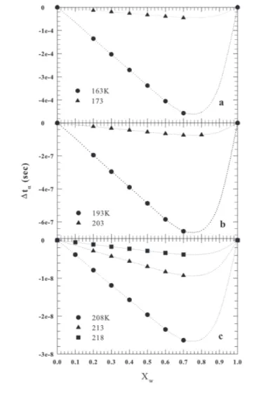
3.4 Δ𝑡_𝛼 vs𝑋_W for 163< 𝑇 < 218 K . . . . 63

3.5 Δ𝑡_𝛼 vs𝑋_W for 296< 𝑇 < 335 K . . . . 64

(8)

3.7 Measured diﬀusion𝐷 data for hydrated lysozyme . . . . 67

3.8 Ratio between diﬀusion data of bulk water and of that in hydrated lysozyme 69 3.9 The thermal behavior of the reorientational correlation time of lysozyme hydration water . . . 71

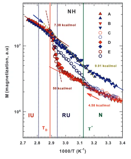
3.10 The hydrodynamic radius for bulk water and lysozyme hydration water . 72 3.11 Arrhenhius reprentation of the magnetization values of lysozyme amide NH groups . . . 75

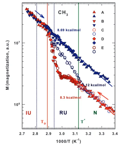
3.12 Arrhenhius reprentation of the magnetization values of lysozyme methyl CH₃groups . . . 76

3.13 Arrhenhius reprentation of the magnetization values of lysozyme me-thine CH groups . . . 77

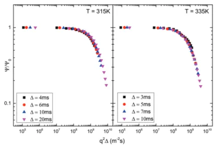
3.14 The normalized echo NMR attenuation as a function of𝑞2_Δ _{. . . .} ₇₉

3.15 The normalized spin-echo amplitude as a function of𝑞2 . . . 80

3.16 Mean square displacement vs diﬀusion time . . . 80

3.17 𝑇 dependence of the power law exponent 𝛼 for hydrated lysozyme . . . 81

4.1 |Δ𝑡_𝛼,𝑚| versus 1000∕𝑇 . . . . 84

4.2 𝑡_𝛼vs𝑋_Wfor all the investigated temperatures . . . 85

(9)

List of Tables

1.1 List of some physical characteristic properties of water phases at 1 atm . 12 2.1 List of selected nuclear species with their properties relevant for NMR . 35

(10)

List of Abbreviations

AR (pure) ARrhenius (behavior)

CS Conformational Constituents

CSA Chemical-Shift Anisotropy

DRLS Depolarized Rayleigh Light Scattering

DSC Diﬀerential Scanning Calorimetry

DSE Debye-Stokes-Einstein

EMCT Extended Mode Coupling Theory

EPSR Empirical Potential Structure Refinement

FID Free Indution Decay

FSDC Fragile-to-Strong Dynamic-Crossover

FST Fragile-to-Strong Transition

FT Fourier Transform

FWHM Full-Width (at) Half-Maximum

GPD Gaussian Phase Distribution (approximation)

H Hydrogen

HB Hydrogen Bond

HDA High-Density Amorphous (Phase)

HDL High-Density Liquid (Phase)

HDS High-Density Structure

HR High-Resolution

HR-MAS High-Resolution Magic Angle Spinning

LDA Low-Density Amorphous (Phase)

LDL Low-Density Liquid (Phase)

LDS Low-Density Structure

LLCP Liquid-Liquid Critical Point

LLPT Liquid-Liquid Phase Transition

MCT Mode Coupling Theory

MD Molecular Dynamics

MRI Magnetic Resonance Imaging

MSD Mean-Squared Displacement

ND Neutron Diﬀraction

NMR Nuclear Magnetic Resonance

PFG Pulsed Field Gradient

PFGSE Pulsed Field Gradient Spin-Echo

PFGSTE Pulsed Field Gradient STimulated (spin) Echo

RF Radio-Frequency

SA Super-Arrhenius (behavior)

SGP Short Gradient Pulse (approximation)

SI Système International (d’unités)

SF Singularity-Free (Scenario)

SLC Stability Limit Conjecture

TE Time (of the) Echo

(11)

TMSC Temperature Modulated Scanning Calorimetry

VD Variable Delay (parameter)

VFT Vogel-Fulcher-Tamman

(12)

Physical Constants

Boltzmann Constant 𝑘_𝐵 = 1.380 648 52(79) × 10−23J K−1

Nuclear Magneton 𝜇_𝑛= 5.05 × 10−27_{A m}−2

Proton’s Gyromagnetic Ratio 𝛾 = 2.675 221 900(18) × 108rad s−1T−1 Reduced Proton’s Gyromagnetic Ratio 𝛾 = 42.58 × 108MHz T−1

(13)

List of Symbols

𝐸_𝑎 activation energy J

𝑚_𝑙 angular quantum number 𝑙 azimuthal quantum number

𝑇_𝐵 boiling point temperature K

𝐻0 constant magnetic field A m−1

𝐷 diﬀusion coeﬃcient m2s−1

𝑆 entropy J K−1

𝑆_{𝐹 𝑇} Fourier transformed signal

𝑇_𝐿 fragile-to-strong dynamic crossover temperature K

𝑇_𝑔 glass transition temperature K

𝑇_𝐻 homogeneous nucleation temperature K

ℎ hydration level

𝑟 interproton distance Å (10−10m)

𝑐_𝑃 isobaric specific heat capacity J g−1K−1

𝑇∗ _{"magic" temperature} _K

𝐵 magnetic field T

𝑔 magnetic field gradient T m−1

𝑚_𝑗 magnetic quantum number

𝑀 (macroscopic) magnetization N m T−1

𝑇_𝑀 melting point temperature K

𝑋MeOH methanol molar fraction 𝑡MeOH

𝛼 water relaxation time s

𝑠_𝑚 molar entropy J K−1mol−1

𝑋 molar fraction

𝑣_𝑚 molar volume m3mol−1

𝐼 nuclear spin quantum number

𝐿_𝑧 orbital angular momentum (along the z axis) N m s

𝑃 pressure Pa (N m−2)

𝑇_𝐷 protein denaturation temperature K

𝑇1 proton spin-lattice (longitudinal) relaxation time s 𝑇2 proton spin-spin (transverse) relaxation time s

𝑡_𝛼 relaxation time s

𝑠 spin quantum number

𝑆_𝑧 spin projection angular momentum along the z-axis N m s 𝑚_𝑠 spin projection quantum number along the z-axis

𝐵0 static magnetic field T

𝑇 temperature K

𝐽_𝑧 total angular momentum (along the z axis) N m s

𝑉 volume m3

𝑋W water molar fraction 𝑡W

𝛼 water relaxation time s

(14)

𝜎 chemical shift

𝜌 density kg m−3

Δ diﬀusion time s

𝛿 duration of the gradient pulse s

Ψ echo attenuation a. u.

𝜙 fluidity Pa−1s−1

𝜉 hydrodynamic radius m

𝜅_𝑇 isothermal compressibility Pa−1(m2N−1)

𝜔0 Larmor angular frequency rad s−1

𝜈0 Larmor frequency s−1

𝜇 magnetic moment N m T−1

𝜌_𝑁 number density of nuclei m−3

𝜏 delay of the gradient pulse s

𝜏_𝜃 reorientational correlation time s

𝜏_𝑐 rotational characteristic correlation time s 𝛼_𝑃 thermal expansion at constant pressure K−1

(15)

Dedicated to those who love and supported me in achieving this

goal.

(16)

Chapter 1

Water and water systems

1.1 Water

Water is the most copious inorganic molecule in the universe after hydrogen and it is essential to life and human activity [1–11]. Since water is absolutely essential to all living things, it should not be surprising that it has been considered a very important topic in both philosophy and science from ancient times. For example, in the VIth_century BC, Thales of Miletus, philosopher, mathematician and astronomer, declared water to be the "principle element" of all things introduced for the first time by Aristotle. Thales claimed that from water all things emerge and to which they return, and, in addition, that all things sooner or later are water. Subsequently, Aristotle agreed that water was the "principle" of biology and thus of all living things. Indeed, all life on Earth needs water to survive (i.e., living organisms require, contain and maintain a balance of water) and/or to fulfill its functional activity. In the human body, water contributes to many biological and physiological functions such as the triggering of enzymatic activity (e.g., water-lysozyme interaction [4, 12, 13] in the human saliva). From the point of view of biology, water acts as a solvent or a solute, and a biomolecule, structuring proteins, nucleic acids and cells [1–5, 14]. Furthermore, water is unique compared to the other substances for all its properties (and anomalies), especially in the supercooled regime [4, 5, 15–17] where water remains liquid below the melting point.

In nature, it is possible to find water in gaseous, liquid and solid phases, and, in particular, water is the only inorganic substance that is liquid at atmospheric pressure and ambient temperature. In these conditions, it is an odorless, tasteless liquid, and appears colorless in small quantities, although it has a hint of blue [1, 7, 18]. Water freezes into ice below 0◦C and boils above 100◦C. Ice also appears colorless, and water vapor is essentially invisible as a gas.

Because of what has just been said, understanding the thermodynamical and dynam-ical properties of water is a challenging research subject in both science (including the fields of physics, chemistry, and biology) and technology. In particular, the focus of this thesis is on biological water, i.e. water located in living systems, and the study of its interaction with substances in aqueous solutions.

1.1.1 The water molecule

The water molecule consist in two hydrogen (H) atoms bonded with an oxygen (O) atom, so its chemical formula is H₂O1(figure 1.1). Each hydrogen is bound to the central oxy-gen atom by a covalent chemical bond, in which a pair of electrons are shared between them. The structure of the molecule is "bent" like, with positive and negative sites lo-cated in diﬀerent places. In fact, the O atom has an average electron density about 10

1_{The molecular composition of water is due to the London scientist Henry Cavendish in 1781,}

(17)

times more intense than the H atoms and this provokes a dislocation of the center of the positive charge (half way between the two hydrogen atoms) on respect with the center of the negative charge (on the oxygen atom). Indeed, a diﬀerent and "partial" positive and negative charge distribution is established, giving rise to a permanent dipole moment. In this way, each molecule of H₂O is electrically neutral, but polar. Polarity is respon-sible for some water’s unique properties. For example, it makes water a "good solvent" allowing it to dissociate ions in salts and greatly bond to other polar substances (e.g., alcohols).

FIGURE1.1: The liquid water molecule. As experimentally determined, a gaseous water molecule has an O–H length of 0.9718 Å and H–O–H angle of 104.474◦, instead in the liquid water molecule these values are slightly greater [7]. Commonly used values for O-H lengths and H-O-H angles in the liquid water molecule are ranged between 0.957 Å and 1.00 Å, and from 104.52◦to 109.5◦, respectively. Note that the H-O-H angle in both liquid and gaseous phase is somewhat less than the tetrahedral angle (109.47◦), because of the lower repulsion between H atoms than between them and the unbonded electrons (lone pairs) of the oxygen

atom [1].

The presence of two lone pairs of electrons in the oxygen atom, in addition to be responsible for example of the H–O–H bond angle (∼ 104.5◦ for the gas phase and ∼ 106◦for the liquid phase) which is smaller than the typical tetrahedral angle of 109.47◦, gives rise to an electrostatic-type bond between water molecules called hydrogen bond.

1.1.2 The hydrogen bond

The hydrogen bond2(HB) establishes in water when a hydrogen atom of one molecule ("proton donor") interacts with the oxygen atom of another water molecule ("proton ac-ceptor").

The hydrogen bond in water can be considered as the sum of an electrostatic part (∼ 90%) and a covalent one (∼ 10%), but, normally, HB is established from a complex com-bination of interdependent interactions [1]. In particular, HBs are not static connections because they switch protons and partners without stop3.

Liquid water is composed by a combination of (i) long, weak and bent HBs, (ii) short, straight and strong HBs, and (iii) hydrogen bonds with many intermediate between

2_{Hydrogen Bonding was first suggested in water by Latimer and Rodebush in 1920 [1, 2, 20, 21] and its}

concept and denomination were developed later by Pauling [22].

(18)

FIGURE 1.2: Hydrogen bond tetrahedron between water molecules in the liquid phase.

(i) and (ii) [7]. When two isolated H₂O molecules come close, a dimer is formed by means of one or two HBs. In the first case (the most energetically favourable one), the structure formed is called linear, otherwise it is cyclic or bifurcated. When several water molecules approach, they assemble trimers and other diﬀerent clusters as a function of their value of temperature and pressure4_{. In fact, when T decreases, the HBs cluster} and form an open tetrahedrally coordinated HB network. In particular, when the T of the stable liquid phase is lowered, HB lifetime and cluster stability increase. Note that, in liquid water, each H₂O molecule can form at most four HBs with surrounding water molecules establishing, indeed, a HB tetrahedrally coordinated network. This structure emerges because each electrons of the lone pairs of the oxygen and each hydrogen of a water molecule can establish a HB with a H atom and two O atoms of diﬀerent water molecules, respectively. This situation is well evident in figure 1.2. Generally, water molecules have the ability to form an extended dynamic HB network with localized and structured clustering.

From the point of view of the binding energy, in liquid water, the H atom is connected to the O atom of the same water molecule by means of a covalent bond (∼ 492 kJ/mol), but has an additional energy of attraction to the oxygen of another water molecule (hydrogen bond enthalpy: ∼ 23 kJ/mol [23]). In particular, this strong attraction (called indeed the hydrogen bond) has an energy strength in liquid water far greater and more directional at room temperature than Van der Waals interaction forces (∼ 5.5 kJ/mol) [1, 7, 11].

Anyway, the physics of hydrogen bond, for its complexity and importance not only in water and aqueous systems, should require a complete treatise [7, 11]. It is really important to stress the fact that H₂O molecules have the tendency to attract each other

(19)

strongly by means of hydrogen bonds. In particular, HB is the principal addresser for the complex phase diagram of water.

1.1.3 Water phase diagram

In nature, water can be found in gaseous, liquid and solid phases5 _{as showed in figure} 1.3, a (P,T) plot that represents the phase diagram6of water.

0 100 200 300 400 500 600 10 1 10 2 10 3 10 4 10 5 10 6 10 7 10 8 10 9 10 10 10 11 10 12 GAS LIQUID SOLID

Cri ti cal Poi nt

(1 atm) Freezi ng Poi nt I h I c XI rhom bi c) (ortho-III V VIII IX XV II VI VII X P r e s s u r e ( P a ) T emperature (K) XI (hexagonal) Tri pl e Poi nt Boi l i ng Poi nt (1 atm)

FIGURE1.3: The (𝑃 ,𝑇 ) phase diagram of water. The black lines repre-sents the phase curves that divide the physical states of water. Freezing, boiling and triple points are reported. The star (⭐) denotes the stan-dard ambient condition. The thirteen forms of ice are also indicated and

separated by light blue lines.

At standard ambient temperature and pressure (marked with a⭐ in figure 1.3) water is a liquid, but it becomes gaseous (i.e., water vapor) if its temperature is increased above 100◦C or solid (i.e., ice) lowering the temperature below 0◦C, at fixed pressure. These "phase transitions" at pressure of 1 atm are denoted with a red line in figure 1.3 that crosses the melting point of ice (or the freezing point of liquid water) at 𝑇_𝑀∼ 273 K and the boiling point of water at𝑇_𝐵∼ 373 K. In particular, the range defined by these equilibrium points corresponds to the stable liquid range. Furthermore, there is a special point at 273.16 K and 611.657 Pa called "triple point" where liquid water, gaseous water and hexagonal ice stably coexist, and where both the melting point and the boiling point are equal.

5_{In thermodynamics, a phase is a region of a system in which all physical properties of a material are}

basically uniform

6_{Phase diagrams illustrate the preferred physical states (phase) of matter at diﬀerent temperatures and}

pressure. Each equilibrium curve (phase line) on a phase diagram denotes a phase boundary and gives the conditions when two phases may stably coexist because these states have the same Gibbs free-energy. In fact, here, just a very small change in temperature or pressure possibly causes a phase transition from one physical state to the other. In particular, where three phase lines join each other, there is a "triple point", when even three phases stably coexist.

(20)

The end point of the phase curve that denotes conditions under which liquid water and its vapor become indistinguishable from each other is the "critical point", defined by a critical temperature𝑇_𝑐 and a critical pressure𝑃_𝑐. At temperatures above𝑇_𝑐 a gas cannot be liquefied.

Anyway, the phase diagram of water is quite rich. For example, as shown in figure 1.3, at low temperatures, in its crystalline state, water is found to exist in thirteen diﬀerent forms, nine of which are stable (ices II, III, V, VI, VII, VIII, X, XI, hexagonal I_ℎ) over a particular ranges of temperature and pressure, and four are metastable (ices IV, IX, XII and cubic I_𝑐). The known ices can be partitioned into the low-pressure ices (I_ℎ, I_𝑐and XI), high pressure ices (VII, VIII and X) and the others (found in the range of moderate pres-sures around 1 GPa). For example, below 273 K and at 1 atm, the stable crystalline state is the so-called Ice I_ℎ. Here each water molecule has four nearest neighbours consitut-ing, as already mentioned before, a regular tetrahedron held (together) by HBs. Because of the strong directionality of the hydrogen bond, this kind of tetrahedrally coordinated network results to be open. It is important to stress that water molecules can form an extended dynamical HB network and this clustering behavior is commonly accepted to be the cause of water anomalous properties.

1.1.4 Anomalous properties of water

Water is characterized by several uncommon thermodynamic and dynamical properties or anomalies that make it a "sui generis" liquid7. So, although it is an apparently simple molecule (see figure 1.1), water shows anomalous and complex behaviors mostly due to its HBs [22, 26, 27], and it seems that life and its processes depend on these anomalous properties [2, 6, 7, 11, 26].

The high cohesion between water molecules due to HBs gives it a high freezing and melting point, and it is because of these that in our planet we find more water in its liquid state. Furthermore, water properties such as its large heat capacity and its high content in organisms permit to more easily control our body temperature. As already mentioned, water has unique hydration properties towards important biological macro-molecules (e.g., proteins) that regulate their structures and biological functions [1, 4, 12, 13] and it is also an excellent solvent due to its polarity, high relative permittivity (dielectric constant) and small size.

Nowadays, over 70 anomalies have been found for water [7]. Figure 1.4 displays a detailed region of the phase diagram of figure 1.3 in which some peculiar properties of water are evinced. In particular, it is noteworthy to attention the supercooled regime in which these anomalies become more evident [16, 25]. At atmospheric pressure, water can be "supercooled" down to its crystal homogeneous nucleation at𝑇_𝐻∼ 231 K, because at this temperature the nucleation rate suddenly increases [16], and it is not possible to find water in its liquid state below this point. In the supercooled regime, water is in a metastable state, a condition of precarious equilibrium in which it is prepared to collapse in its crystalline state when a perturbation is applied. Note that the process of supercooling depends on the purity of water and the freedom from nucleation sites in the cooling of liquid water [16]. Like any other liquid, water can be also superheated over its boiling point, without going through a phase transition, until ∼ 553 K. As seen for the supercooled water, the rate of nucleation control the superheating process too. Thus it is possible in principle to have liquid water within a huge temperature range (231–553 K).

7_{The properties of water are seen to be anomalous on respects the materials used in the comparison and}

the interpretation of the term "anomalous" [7]. In the past decades, a lot of articles have been published on water anomalies, even an historical study [24] Today, water scientists agree that water is the most anomalous substance [25].

(21)

These metastable limits are not thermodynamic but kinetic in nature; so, they occur only when the nucleation time is shorter than the experimental observation time.

150 200 250 0.1 0.15 0.2 0.25 T M Supercooled Region Ice II Ice III Ice I TMD T H

"No Man's Land"

W idom Line Liquid-Liquid Critical Point T x LDL LDA HDL HDA P r e s s u r e ( G P a ) T emperature (K)

FIGURE1.4: The (𝑃 ,𝑇 ) phase diagram of water in the frame of its poly-morphism and the supercooled regime (see the text for more details). At ambient pressure, metastable supercooled water is located on the phase diagram between the melting temperature𝑇_𝑀∼ 273 K and the homo-geneous nucleation temperature𝑇_𝐻∼ 231 K. The amorphous phases, LDA and the HDA, and the LDL and HDL phases are reported together with the melting𝑇_𝑀, the maxima density TMD and the homogeneous nucleation temperature𝑇_𝐻and the crystallization𝑇_𝑋loci. The Liquid-Liquid critical point and the Widom line are also reported and they will

be described later.

Liquid water experiences a glass transition8 when the cooling rate is very high (∼ 106K/s) [16, 28, 29] becoming an amorphous solid at the temperature𝑇_𝑔∼ 130 K9[31, 32]. So, below the glass transition temperature𝑇_𝑔, water exists as glass; above this tem-perature, it becomes a highly viscous fluid that crystallizes spontaneously into cubic ice (I_𝑐) at𝑇_𝑋∼ 150 K.

The region between𝑇_𝐻 and𝑇_𝑋 represents the temperature range where liquid water is not easily accessible experimentally, known as “No Man’s Land” of the phase diagram (see figure 1.4).

Unlike most other substances, glassy water is characterized to be "polyamorphic"10 at least in two diﬀerent forms, known as low-density amorphous water (LDA) and high-density amorphous water (HDA), separated by a first-order phase transition and that can

8_{The glass transition is a "dynamic arrest" phenomenon (DA) in amorphous materials from a "viscous"}

state to a noncristalline "glassy" state by cooling fast enough to avoid crystallization [16]. In such condi-tions, the units constituting the system, switching from single molecules to clusters of molecules, interact more strongly and their dynamics slows down considerably: therefore, it is observed a drastic change of the physical properties of the system. This phenomenon is marked by the glass transition temperature𝑇_𝑔that is diﬀerent for each material. In fact, this temperature depends on the strength of the interparticle interactions, i.e., the "bonds" that are being broken as the particles rearrange.

9_{It has been argued that the glass transition temperature for water is higher than about 130 K [30]} 10_{Polyamorphism is the phenomenon that predicts for a substance its existence in several amorphous}

(22)

be transformed one into the other by tuning the pressure [4, 15, 29, 33–35]. This "poly-morphic glass transition" is combined with a large and sharp variation in the system volume when thermodynamic parameters such as temperature change infinitesimally.

This polyamorphism of water in conjunction with HB networking suggest that liquid water can also be polymorphous, i.e., a mixture of a high-density liquid (HDL) and a low-density liquid (LDL) [16]. In the HDL form, which rules for high temperatures, the local tetrahedrally coordinated structure is not perfectly established, but in the LDL phase, a more open “ice-like” HB network arises.

Some of the most known anomalies of water at atmospheric pressure are (i) the max-imum of the density 𝜌 at ∼ 277 K (figure 1.5), (ii) the zero value of the coeﬃcient of thermal expansion𝛼_𝑃 at ∼ 277 K (figure 1.6a), (iii) the minimum of the isothermal com-pressibility𝜅_𝑇 at ∼ 319 K (figure 1.6b), and (iv) the minimum of the isobaric specific heat capacity𝑐_𝑃 at ∼ 309 K (figure 1.6c).

The density maximum is the reason of the water expansion on heating or cooling at ∼ 277 K. Technically, this maximum at 4◦C is caused by the contrasting eﬀects due to the increasing of temperature that provides both structural collapse (i.e., an increase of density) and thermal expansion (i.e., a lowering of𝜌) [7].

255 270 285 300 315 330 345 360 965 970 975 980 985 990 995 1000 ( k g / m 3 ) T emperature (K) Maxim um at ~ 277 K

FIGURE1.5: The temperature dependence of liquid water density𝜌 at atmospheric pressure. The density maximum is well evident at ∼ 277

K. Data taken from [36–38].

At higher temperatures there are more high-density structures (HDS), whereas at lower temperatures there is a higher concentration of low-density structures (LDS). In-creasing the temperature, the "transition" from LDS to HDS occurs with positive changes in both enthalpy and entropy due to the greater hydrogen bond bending and the less or-dered structure, respectively.

The central property of the water density anomaly is the locus of temperatures at which the density is maximum at fixed pressure that is known as temperature of maximum density (TMD). Note that, if the pressure is positive, this locus has a negative slope in the (𝑃 ,𝑇 ) plane. This happens because when 𝑇 is lowered, the compressibility of liquid water increases [29].

(23)

The density maximum results in several important features that aﬀect life. For exam-ple, the freezing of rivers, lakes and oceans is from the top down, so permitting survival of the bottom ecology [7].

In addition, at atmospheric pressure, liquid water shows another peculiarity, that is the modulus of its response functions11increases sharply on reducing the temperature, diverging towards the supercooled region [16, 29]. Figure 1.6 shows the𝑇 dependence of some liquid water response functions at 1 atm.

-1.0 -0.5 0.0 0.5 0.5 0.6 0.7 0.8 255 270 285 300 315 330 345 360 75 80 85 90 P ( 1 0 -3 K -1 ) Zero at ~ 277 K a) ln P P B S V T kTV 2 ln ln T T B V P kVT b) T ( G P a -1 ) Minimum at ~ 319 K Minimum at ~ 308 K c P ( J / m o l * K ) Temperature (K) 2 P P B S S c T T k c)

FIGURE1.6: The temperature dependence of liquid water a) thermal ex-pansion coeﬃcient𝛼_𝑃, b) isothermal compressibility𝜅_𝑇 and c) isobaric specific heat𝑐_𝑃 at atmospheric pressure. Equations for each response

function are also reported. Data taken from [36, 39].

The first derivative of the natural logarithm of density𝜌 with respect to the tempera-ture𝑇 at constant pressure 𝑃 determines the coeﬃcient of thermal expansion 𝛼_𝑃

𝛼_𝑃 = − ( 𝜕ln𝜌 𝜕𝑇 ) 𝑃 (1.1)

11_{In thermodynamics, the response functions represent the variation of a system’s thermodynamic}

(24)

that can be also express as the cross-correlation between𝛿𝑆 and 𝛿𝑉 , the entropy and volume fluctuations, respectively:

𝛼_𝑃 = ⟨𝛿𝑆𝛿𝑉 ⟩

𝑘_𝐵𝑇 𝑉 (1.2)

Note that𝛿 represents the variation about the mean value of a thermodynamic quan-tity,𝑘_𝐵 is the Boltzmann constant and𝑉 being the mean value of 𝛿𝑉 for a fixed number of molecules. As shown in figure 1.6a, 𝛼_𝑃 is zero before the melting point, at ∼ 277 K, location of the already described maximum value of water density. It is noteworthy that the locus of points where𝛼_𝑃 changes its sign coincides with the TMD. In particular, lowering the temperature, the coeﬃcient of thermal expansion becomes negative, and it is a very anomalous behavior compared with normal liquids that remain positive with an almost linear dependence on temperature. In fact, liquids expand on heating, while water contracts with increasing temperature for𝑇 < 277 K.

The variation of the natural logarithm of the density𝜌 with respect to the natural logarithm of pressure𝑃 at constant 𝑇 defines the isothermal compressibility 𝜅_𝑇

𝜅_𝑇 = ( 𝜕ln𝜌 𝜕ln𝑃 ) 𝑇 (1.3) that is proportional to the microscopic volume fluctuations𝛿𝑉 :

𝜅_𝑇 = ⟨

(𝛿𝑉 )2⟩

𝑘_𝐵𝑇 𝑉 (1.4)

The𝑇 dependence of the isothermal compressibility is strictly related to the slope of the TMD in the (𝑃 ,𝑇 ) plane [40]. In a normal liquid, reducing the temperature, 𝜅_𝑇 decreases, whereas in water, as pointed out in figure 1.6b, it increases sharply at𝑇 = 319 K towards lower temperatures. In addition, from experimental data [41], the lower temperature behavior appears to be described by a power law:

𝑌 (𝑇 ) = 𝐴 ( 𝑇 𝑇_𝐿 − 1 )_𝛾 (1.5) where𝑌 is a thermodynamic quantity, A its amplitude and 𝛾 is a critical exponent associated to the divergence of𝑌 at the singular temperature 𝑇_𝐿.

The variation of the entropy𝑆 with respect to 𝑇 at constant 𝑃 multiplied by the temperature determines the isobaric specific heat𝑐_𝑃:

𝑐_𝑃 =𝑇(𝜕𝑆 𝜕𝑇

)

𝑃 (1.6)

that is, microscopically, proportional to entropy fluctuations𝛿𝑆 at fixed pressure:

𝑐_𝑃 = ⟨

(𝛿𝑆)2⟩

𝑘_𝐵 (1.7)

in which it has been considered the number of moles𝑛 equal to 1. The isobaric specific heat of water behaves like its𝜅_𝑇, but the increase starts at𝑇 = 308 K (see figure 1.6c). In fact, the water structure equilibrium shifts towards LDS as the temperature is reduced, causing great changes in entropy fluctuations. In particular, at supercooling temperatures where a much larger shift arises,𝑐_𝑃 increases a lot and follows a power law similar to that of equation 1.5.

Lowering the temperature, the variation of water response functions appears more pronounced (and less when a pressure is adopted [29]), and, in particular, Speedy and

(25)

Angell [42] could assert that the characteristic relaxation times and the thermodynamic response functions of water diverge at a peculiar temperature𝑇_𝐿= 228 K. Note that this temperature lies in the already defined "No Man’s Land". So, experiments performed within this region could be very useful for understanding the physical origin of this ap-parent singular temperature 𝑇_𝐿, giving possible explanations of many open questions concerning the properties of supercooled water [43].

Water is characterized even by peculiar dynamical properties because of the compe-tition at equilibrium between HB and Van der Waals interactions. Transport coeﬃcients such as viscosity𝜂 (or structural relaxation time 𝑡_𝛼) and translational diﬀusion𝐷 show a particular trend at lower temperatures when the LDS predominate.

In water, the shear viscosity𝜂12is marked by a large cohesivity due to its extensive 3D hydrogen bonding (figure 1.7 (top)). In fact, HBs tend to form more ordered (and symmetrical) structures, whereas the van der Waals interactions (together with the ther-mal energy) have the inclination to assemble more packed disordered structures (more similar to those of normal liquids) in conjunction with the thermal energy. As mentioned before, reducing the temperature, HBs win over van der Waals interaction resulting in an increase of the number of LDS with respect to HDS [44]. In this way, the majority of clusters are larger and their presence leads to an increase of viscosity due to a reduction of the movement.

As usually happens when pressure is applied to a liquid, its molecules are forced to stay together and holes and defects vanish increasing the viscosity of the liquid. In liquid water, the application of a pressure provokes the break of the tetrahedral HB network (i.e., the LDS), that is the molecular mobility increases. In fact, the LDS reduce its number and size under pressure, and water will become more like a normal liquid. The variation of the shear viscosity with respect to pressure is shown in figure 1.7 (bottom). It looks clear that it becomes more pronounced at low temperature, where the number of LDS is bigger [45].

In particular, viscosity is connected to the already mentioned glass transition tem-perature𝑇_𝑔. It is possible to define𝑇_𝑔 as the temperature at which viscosity reaches the value of 1013_{poise [47]. Using Angell’s interpretation [28, 30, 48], the "fragility" of a} glass-former is described in terms of the deviation of its viscosity and relaxation time𝑡_𝛼 temperature dependence from simple Arrhenius behavior. A supercooled liquid is termed "fragile" when it is characterized by a highly non-Arrhenius temperature dependence of 𝑡_𝛼; whereas, a supercooled liquid is "strong" when its viscosity shows a temperature de-pendence close to the Arrhenius law. A fragile liquid changes a lot its structure with temperature; on the contrary, the structure of a strong liquid changes a little when tem-perature changes. Furthermore, strong liquids become fragile on compression, and this behavior can be related to a polyamorphism in the glassy state. The pure Arrhenius (AR) behavior belonging to strong liquids is identified by an activation energy𝐸_𝑎that is temperature-independent. In this case, the viscosity𝜂 is usually written as

𝜂 = 𝐴 exp ( _𝐸 𝑎 𝑘_𝐵𝑇 ) (1.8) where A is just a temperature-independent factor, like𝐸_𝑎, and𝑘_𝐵is the Boltzmann’s constant. On the other hand, the fragile or Super-Arrhenius (SA) behavior was usually treated with a Vogel-Fulcher-Tamman (VFT) equation [49–51] in which, lowering the temperature, the eﬀective activation energy value increases. In this frame, the viscosity is represented by the following law

12_{The shear viscosity of a liquid is established by the cohesiveness of molecules, i.e., the forces holding}

(26)

0 2 4 6 8 10 255 270 285 300 315 330 345 360 -30 -25 -20 -15 -10 -5 0 ( c P ) P ( p s ) Temperature (K)

FIGURE1.7: (Top) Temperature dependence of water shear viscosity at atmospheric pressure and (bottom) its variation with respect to pressure

as a function of temperature. Data taken from [45, 46].

𝜂 = 𝐴 exp ( 𝐵 𝑇 − 𝑇0 ) (1.9) where A and B are factors independent from𝑇 and 𝑇₀is the "ideal" glass transition temperature (known as the Kauzmann temperature [30]) which is kinetic in nature. The power law approach has a more physical meaning with respect to the VFT method. In fact, water is one of the most known and studied fragile liquid above 235 K [52], and, in particular, it seems that its viscosity follows a power law diverging at about 228 K [42]. Anyway, the temperature dependence of 𝜂 must change from its power law form below 235 K because of the presence of𝑇_𝑔at below 180 K. So, it has been proposed [53, 54] that supercooled water experiences a "fragile-to-strong" transition (FST) around the crossover temperature of 228 K, and that it is due to an end point in the formation of a hydrogen bonded tetrahedral network structure [52].

Another transport parameter of great importance is the translational diﬀusion𝐷. It represents the molecular transport driven by the kinetic energy and it is also related to the size of the diﬀusing object and the viscosity of the system through the Stokes-Einstein (SE) relation

(27)

𝐷 = 𝑘𝐵𝑇

6𝜋𝜂𝜉 (1.10)

in which𝜉 is the hydrodynamic radius for a spherical molecule. It has been reported that this relation breaks down at temperatures not far above the glass transition temper-ature𝑇_𝑔 [55] and also that, for supercooled water, the SE is no longer valid well above 𝑇_𝑔, occurring at about 225K [56, 57]. The𝑇 -dependence of 𝐷 in water was shown in figure 1.8 [58, 59]. In particular, by means of Pulsed Field Gradient Spin-Echo (PFGSE) Nuclear Magnetic Resonance (NMR), Price et al. were able to reach 238 K and they found that, lowering the temperature, the diﬀusion behavior became non-Arrhenius and can be described by a VFT law like that of equation 1.9.

240 255 270 285 300 315 330 345 360 375 1E-10

1E-9 1E-8

Price et al. Simpson and Carr

D ( m 2 / s e c ) T emperature (K)

FIGURE 1.8: Temperature dependence of supercooled water self-diﬀusion in a lin-log plot. Data taken from [58] (dark blue circles) and

[59] (light blue squares).

In table 1.1 are listed some of the most known thermal properties of water at 1 atm.

TABLE 1.1: List of some physical characteristic properties of water phases at atmospheric pressure [37].

Temperature𝑇 Density 𝜌 Specific Heat C_𝑝 Thermal Cond.𝑘 Viscosity 𝜂

(K) (kg/m3₎ _(J/mol_⋅K) _(W/m_⋅K) _(cP)

liquid 293.16 998.21 75.38 0.56 1.79

vapor 373.16 0.6 37.47 0.03 0.01

Note that Mallamace et al. [60] presented a very complete overview about transport properties and anomalies of water, especially in the supercooled region.

1.1.5 Theoretical models and scenarios

In order to comprehend the anomalous and chemico-physical properties of liquid water, diﬀerent theoretical models have been developed. However, we will detail only the recent three most plausible interpretations [29].

(28)

FIGURE1.9: The (𝑃 ,𝑇 ) planes representing the thermodynamic behav-ior of water predicted by three competing theories, a) the stability limit hypothesis, b) the percolation picture (and singularity-free hypothesis), and c) the liquid–liquid phase-transition hypothesis. Here𝐶 denotes the known critical point,𝐶′indicates the hypothesized second critical point, and𝑇_𝑠 shows the locus of spinodal temperatures. 𝐺 and 𝐿 denote the low-density and high-density fluid phases that exist below𝐶, whereas LDL and HDL denote the low-density and high-density liquid phases

that exist below𝐶′. Figure adapted from [61].

Stability limit conjecture

In 1976, Speedy and Angell hypothesized that the temperature𝑇_𝐿= 228 K may be con-sistent with the limit of mechanical stability for the supercooled liquid water [42]. On the basis of this assumption, in 1982 Speedy [62] proposed an "interpretation" to explain the thermodynamics of metastable water, the Stability Limit Conjecture (SLC), according to which the increment in response functions for supercooled water is generated by the approach to the spinodal curve13, the locus of the points where superheated liquid water becomes unstable with respect to the vapour phase (𝑇_𝑠curve in figure 1.9a). In normal liquids, the spinodal starts at the liquid-gas critical point and, in the (𝑃 ,𝑇 ) plane, it has a positive slope and decreases monotonically with decreasing𝑇 along a path lying below the liquid-gas coexistence curve. According to Speedy’s interpretation, in liquid water, the spinodal is curved inwards instead: it has a minimum at negative𝑃 and, decreasing 𝑇 , it passes back to positive 𝑃 .

In particular, the spinodal can be considered a locus of diverging density and entropy fluctuations [29], so its retracing character would indeed demonstrate some of the exper-imentally observed water’s anomalies. In fact, the maximum in the density𝜌 of water at 277 K and the minimum in the isothermal compressibility𝜅_𝑇 at 319 K are possibly manifestations of spinodal-induced thermodynamic singularities occurring in the super-cooled region. From a thermodynamic point of view it appears that the slope in the (𝑃 ,𝑇 ) plane of a spinodal curve must shift sign upon meeting a line along which the thermal expansion coeﬃcient𝛼_𝑃 becomes zero as showed in figure 1.6a [62, 63]. This line is the already mentioned temperature of maximum density (TMD) that is the locus of temper-atures at which the density is maximum at fixed pressure. Therefore, for liquids with a density maximum such as water, the most physically plausible way for the TMD line to terminate is at an intersection with a spinodal line [63]. But, the situation in which it is possible the intersection in the (𝑃 ,𝑇 ) plane of a positively sloped spinodal line with

13_{The liquid spinodal line, or simply spinodal, designates the limit of stability of the (metastable) liquid}

(29)

a negatively sloped TMD line involves that the liquid spinodal has a minimum at the intersection point [62]. So, at𝑇 less than that of the intersection point, the spinodal is negatively sloped and will occur at higher𝑃 as 𝑇 decreases. Since the intersection of the TMD and spinodal lines is in general expected to occur in the negative𝑃 region of the (𝑃 ,𝑇 ) plane, the spinodal curve 𝑇_𝑠changes from negative to positive𝑃 as 𝑇 decreases, as predicted by the SLC, and illustrated in figure 1.9a.

All the considerations done before allow to predict the behavior of the spinodal line near to specific points, such as its intersection with the TMD line. Anyway, the SLC does not provide informations on the specific shape of the spinodal in the entire (𝑃 ,𝑇 ) plane. The real lack of this interpretation is just in the retracing of spinodal to positive pressure that, e.g., can generate another lower (implausible) critical point for the vapour–liquid transition [29]. To investigate this evidence, several simulation studies have been per-formed. For example, Sastry et al. [64], Sasai [65] and Borick et al. [66], using lattice models with directional interactions, demonstrated that the intersection of the TMD and the spinodal causes the latter to retrace. However, the spinodal does not reach positive pressure and it is replaced by a locus of limits of stability of the supercooled liquid with respect to the solid phase. Furthermore, Poole et al. [67], by means of molecular dynam-ics (MD) simulations found that the spinodal of liquid water is found to be not reentrant and that the TMD line changes slope in the metastable region of the phase diagram at negative pressure.

Singularity-free scenario

Another hypothesis explaining water anomalies is the singularity-free (SF) scenario (fig-ure 1.9b). In this interpretation, the increases in water response functions upon super-cooling (figure 1.6) are illustrated as a consequence of the existence of density anomalies [40, 68]. As an example, Sastry et al. [40] proved that the increment of𝜅_𝑇 on cooling below a negatively sloped TMD line is a requirement of thermodynamics, as stated in the following equation:

(_𝜕𝜅 𝑇 𝜕𝑇 ) 𝑃 ,TMD = 1 𝑣 𝜕2_𝑣 𝑚 𝜕𝑇2 ( 𝜕𝑃 𝜕𝑇 ) TMD (1.11)

where𝑣_𝑚denotes the molar volume and the subscripts "P" and "TMD" indicates that the derivatives are calculated at constant pressure along the TMD locus. Equation 1.11 reports how the temperature dependence of𝜅_𝑇is related with the slope of the TMD line in the (𝑃 ,𝑇 ) plane. Along the TMD line, since 𝜕2𝑣_𝑚∕𝜕𝑇2> 0, the signs of (𝜕𝜅_𝑇∕𝜕𝑇 )_{𝑃 ,TMD} and (𝜕𝑃 ∕𝜕𝑇 )_TMDin equation 1.11 are the same. Consequently, if the TMD has negative slope in the (𝑃 ,𝑇 ) plane, therefore the isothermal compressibility will increases on cool-ing. Thus, in an anomalous liquid such as water, the increase of𝜅_𝑇 upon isobaric cooling is inseparably related to the presence of a negatively sloped TMD.

So in the SF scenario, an increase of compressibility in water is only a thermody-namic requirement and not a priori evidence of any singular behavior as confirmed by Sastry et al. [40] with their lattice model simulation. This model may be viewed as a thermodynamic realization of some basic features of the percolation model of Stanley and Teixeira [69], which indeed predicts the presence of compressibility maxima at low temperatures, i.e., no thermodynamic singularities.

Furthermore, the model explains all the water anomalies in the same way. For exam-ple, the coeﬃcient of thermal expansion𝛼_𝑃 is related to𝜅_𝑇 by the equation:

(30)

(_𝜕𝜅 𝑇 𝜕𝑇 ) 𝑃 = − (_𝜕𝛼 𝑃 𝜕𝑃 ) 𝑇 (1.12) indicating that it increases in magnitude (having a negative sign) on increasing pres-sure but remains finite, without displaying any singularities. Equation 1.12 further sug-gests that the locus of extrema of𝜅_𝑇 with respect to𝑇 along isobars coincides with the locus of extrema of𝛼_𝑃 with respect to𝑃 along isotherms [68]. In particular, Sastry et al. [40] reveal that, on lowering the temperature, liquid water structure equilibrium passes continuously from HDS to LDS (or from High Density Liquid (HDL) to Low density Liquid (LDL)). On the other hand, their model yields two first-order phase transitions. In the low-temperature transition, the phase with higher density also has higher entropy, and hence the transition line has negative slope in the (𝑃 ,𝑇 ) plane [70]. This leads to the last scenario that will be presented in the next section.

Second critical point and liquid-liquid transition

The second critical point interpretation was formulated in 1992 by Poole et al. [70]. It ascribes the anomalous properties of supercooled water to the presence of a metastable, low-temperature liquid-liquid critical point (LLCP), already mentioned in figure 1.4 and indicated with 𝐶′ in figure 1.9c, that is associated with a liquid-liquid phase transition (LLPT) between low-density liquid (LDL) and high-density liquid (HDL) phases.

This hypothesis indeed furnishes a thermodynamically consistent perspective on the global phase behavior of metastable water linking the anomalies of supercooled water to the observed first order transition between LDA and HDA that terminates at the sec-ond critical point above which the two metastable forms of amorphous water become indistinguishable [70]. It is well known that in proximity of a critical point, fluctuations between two closing phases are more accentuated. These enhanced fluctuations influence the properties of liquid water leading to anomalous behavior. Therefore, the already men-tioned experimentally observed sharp increases in liquid water response functions upon cooling are the macroscopic manifestation of the increased fluctuations (equations 1.2, 1.4 and 1.7) associated with this critical point. In particular, in this interpretation, the transition between a denser, disordered phase and a less dense but more structured phase involves discontinuities of volume and entropy: it is a first-order phase transition. Be-cause the high-density phase is also the one with the largest entropy, the phase transition locus is characterized by a negative slope in the (𝑃 ,𝑇 ) plane, and the critical point asso-ciated with this transition corresponds to the temperature above which (and, unusually, the pressure below which) is impossible to distinguish the coexisting phases (figure 1.4). MD simulations were very useful to follow and understand the metastable phases of liquid water and many potentials have been developed and used to reproduce and un-derstand water properties. In 1974 Stillinger and Rahman, using ST2 potential for water, were able to emulate water pair correlation and intermediate scattering functions obtained experimentally [71]. In the 90’s, Poole et al. performed several works on this topics us-ing both ST2 and TIP4P potentials for water [67, 70]. Accordus-ing to ST2 model, the LDA phase possesses sharp inflections in which the volume changes abruptly, suggesting the existence of a first-order phase transition between two amorphous solid forms [70]. Fur-thermore, the response functions of water investigated with the ST2 model increase in the supercooled region in qualitative agreement with experimental observations. The use of TIP4P potential for water furnishes similar results, but adding a contradiction with the stability limit conjecture [67, 72]. In fact, studying the behavior of the liquid spinodal and its relationship to the TMD, Poole et al. found that the TMD retraces towards lower

(31)

temperatures at negative pressure, and does not intersect the spinodal. So their calcu-lated spinodal shows a monotonic positive slope in the (𝑃 ,𝑇 ) plane and does not retrace towards positive pressure, in contrast with the SLC scenario. Anyway, because of the substantial numerical uncertainties associated with finite-size effects which affect com-putational studies, the location of the second critical point is different depending on the model used. In fact, the ST2 model predicts that this occurs at approximately 235 K and 2 kbar [73], whereas the TIP5P model predicts it at approximately 218 K and 3.2 kbar [74].

Mishima and Stanley [75] gave the first important experimental support to the second critical point scenario. In particular, they have studied water droplets with diameters of the order of 1-10𝜇m at high pressures. In such small volumes, nucleation of secondary ice phases following melting in the supercooled regime is kinetically suppressed. So they measured the melting curve of metastable ice IV discovering that this locus experiences a sharp change of slope in the region where it would intersect the presumed line of first-order liquid-liquid phase transitions. It was just this sudden change in the melting curve slope to be attributed to a change in nature of the liquid phase into which the solid melts. This concept is expressed by the Clausius-Clapeyron equation:

d𝑃 d𝑇 =

Δ𝑠_𝑚

Δ𝑣_𝑚 (1.13)

in which d𝑃 ∕d𝑇 indicates the slope of the melting curve in the (𝑃 ,𝑇 ) plane, and Δ𝑣_𝑚 and Δ𝑠_𝑚 denote the diﬀerence in volume and molar entropy, respectively, between the coexisting liquid and solid phases. Furthermore, Mishima and Stanley predicted a low-temperature critical point at approximately 220 K and 1 kbar for supercooled water [75] (figure 1.9c). However, because of the proximity between homogeneous nucleation locus and the first-order transition line, these experiments did not completely clarify the situation.

In the past years, new light was shed on this hot topic. Following the idea of con-fining water, Chen et al. [53, 76, 77] have studied the dynamics of water contained in laboratory synthesized nanoporous silica matrices MCM-41-S with pore diameters of 18 and 14 Å. In this frame, crystallization can be avoided and water can be studied in its liquid state well below 235 K (𝑇_𝐻). In their work, they interpreted the sharp change in the thermal behavior of the average translational relaxation time at 𝑇 = 225 K as the predicted fragile-to-strong liquid-liquid transition. Furthermore, Liu et al. [76] showed that the L-L transition temperature decreases steadily with an increasing pressure, until it intersects the 𝑇_𝐻 line of bulk water at a pressure of 1600 bar. Above this value of pressure, it is no longer possible to distinguish the characteristic feature of the FST. This end point seems to coincide just with the hypothesized second critical point (figures 1.4 and 1.9c). In the (𝑃 ,𝑇 ) plane showed in 1.4, the continuation of L-L transition locus at pressure lower than that of the critical point is called Widom line and coincides with the locus of specific heat maxima, being a critical isochore. Xu et al. [78], by means of MD simulations, found a correlation between the F-S dynamic crossover and the Widom line. In particular, as stated by the Adams-Gibbs theory [79], they evidenced a possi-ble thermodynamic-dynamic relation, in this case between the LLPT and the fragile-to-strong dynamical transition. In particular, this correlation is given by the temperature 𝑇 ≃ 225 K that is called 𝑇_𝐿 and represents both the temperature of the FST and the Widom line temperature (𝑇_𝑊). Recently, Xu et al. [80] review the recent experimental and theoretical progresses on the study of the LLPT in water.

(32)

1.2 Water interacting with other systems

As already stated in 1.1, water has some unusual and important physical and chemical properties, playing a very essential role as a solvent and sustaining the biochemistry of life [1–5, 14]. In fact, over the past three decades, water is not longer considered only as a simply "life’s solvent", but indeed as a "matrix of life" that actively interacts with biomolecules. Water may be considered as a biomolecule in the sense that aggregates of H₂O molecules accomplish delicate biochemical tasks in their interaction with biosys-tems.

Water is called the "universal solvent"14_{because more substances can be dissolved in} water than in any other chemical. In fact, much of life’s chemistry takes place in aqueous solutions, or solutions with water as the solvent. Anyway, the attribute "universal" is not entirely accurate, since there are some substances (such as oils) that do not dissolve well in water. Water’s behavior as a solvent depends on its polarity and the response of its hydrogen-bonded network to the presence of an intruding solute particle [1].

H₂O is an extremely "good solvent" for ions allowing their dissociation in salts and greatly bond to other polar substances (e.g., alcohols). In particular, this is a result of water’s polarity and high dielectric constant, which enables it to screen the Coulombic potential of ions. In the same way, water is an eﬃcient solvent for biomolecular poly-electrolytes such as proteins [1]. As a polar species, water is good at dissolving polar molecules engaging in favorable Coulombic interactions with ions and other polar so-lutes. On the contrary, is a "bad solvent" for non-polar molecules. In fact, non-polar molecules stay together in water because the strong attractive forces that water molecules generate between each other are more intense than the Van der Waals interactions with non-polar molecules. When a polar compound is inserted in aqueous solution, it is sur-rounded by small sized water molecules that constitute an interface called hydration shell. In this frame, two diﬀerent types of substances can be distinguished: (i) hydrophilic ("water-loving") polar substances that will mix well and dissolve in water, and (ii) hy-drophobic ("water-fearing") non-polar substances, that do not mix well in H₂O.

These non-polar molecules are called hydrophobes and usually have a long chain of carbons that do not interact with water. This tendency of water to exclude hydrophobes is named "hydrophobic eﬀect" [81, 82]. In fact, when a hydrophobe is dropped in water, higly dynamic HBs between liquid water molecules will be broken to make room for the hydrophobe. So, hydrophobic solutes in water experience a force that causes them to aggregate. It seems clear that this hydrophobic interaction is in some way responsible for several important biological processes [83], e.g., the folding of proteins. In addition to proteins, there are many other biological substances that rely on hydrophobic inter-actions for its survival and functions, like the aggregation of phospholipids into bilayer membranes in every cell of human body. Particularly interesting is the case of the inter-action of water and amphiphiles, such as methanol.

Here, the role of biological water in its interaction with several biosystems will be highlighted.

1.2.1 Water-methanol solutions

Small amphiphiles in solution with water can be used as "model systems" to analyze water HB interactions and the consequent HB networks [84]. Amphiphilic or amphi-pathic molecules can be considered approximately as linear molecules constituted by a hydrophobic terminal groups and a hydrophilic head. When such "surfactant" molecules

14_{A solvent is a substance that can dissolve other molecules and compounds, which are known as solutes.}