Для цитирования: Экономика региона. — 2015. — №3. — С. 114-122 For citation: Ekonomika regiona [Economy of Region], — 2015. — №3. — pp. 114-122 doi 10.17059/2015-3-10 UDC: 314.17 G. Betti а), E. Caruana b), S. Gusman b), L. Neri a)
a) University of Siena (Siena, Italy) b) National Statistics Office (Valletta, Malta)
economIc Poverty and InequalIty at regIonal level
In malta: focus on the sItuatIon of chIldren
1This paper performs an economic poverty and inequality mapping of three children age categories in Malta; it consists in the first attempt based on income from the EU-SILC survey and Census data. From a policy-making point of view, the availability of such key economic indicators at locality level certainly pro-vides a valuable tool in assessing the effectiveness of national strategies and in identifying areas that need to be targeted by new policies; in fact sample surveys alone cannot provide reliable information at such a fine level of detail, while national censuses are not designed to and cannot be extended to cover specific topics such as economic poverty and inequality. Thus, the merging of the two sources provides policy-makers with a new insight into the differences between localities. There are also benefits of a technical nature, particu-larly in terms of sampling strategies, that can be derived from this study. Through such an exercise it is pos-sible to identify economic homogeneity and/or heterogeneity among households with children in different lo-calities: this is useful when defining strata for sampling design for surveys aiming at studying other economic phenomena relating to children.
Keywords: economic poverty mapping among children, Malta, sampling strategies on economic surveys 1. Introduction
Economic poverty and inequality maps are spa-tial descriptions of the distribution of poverty and inequality; for their construction, living stand-ard information covering consumption expend-iture are needed. Generally censuses do not col-lect expenditure information, so poverty esti-mates are not computable even in the census year. On the other hand, living standard surveys gen-erally cover consumption, however, do not nor-mally permit sufficiently fine disaggregation be-cause of the limited sample size. In order to fill this gap, the World Bank has invested in a meth-odology for generating small area economic pov-erty and inequality measures, thereby permitting the construction of poverty and inequality maps. The methodology, developed by Elbers, Lanjouw and Lanjouw [1], has been applied to a substan-tial number of developing countries, and in many cases the results obtained have been used by gov-ernments to allocate financial resources.
The scope — and the original contribution of this paper — consists in the first attempt of im-plementing an economic poverty and inequality mapping based on income (instead of consump-tion expenditure) from the European Union — Statistical on Income and Living Conditions (EU-1 © Betti G., Caruana E., Gusman S., Neri L. Text. 2015.
SILC) survey and Census data. Moreover, the at-tention is focussed on three age group categories of children, since they are often the most affected by economic poverty.
Statistics on children are therefore extremely important for policy makers, in order to propose ad hoc policies, to combat and eradicate problems such as famine, poverty, exclusion form education, social life, etc., and in order to monitor the effec-tiveness of already undertaken policies. Statistics on children are very important also in developed countries and particularly in the European Union. Information about the economic status where chil-dren live, their health status, their involvement in labour activities, their possible social exclusion, the general condition of immigrated children or chil-dren born in a EU country from immigrated parents are extremely useful information. In the former EU —15 countries, the quality of such data has reached a very high standard and the Commission has the goal to standardise and harmonise this quality level among the current EU-28, including Malta.
The basic idea is to estimate a linear regression econometric model with local variance compo-nents using the information from the smaller and richer data sample, in the Maltese SILC conducted in 2005, including some aggregate information from the Population and Housing Census or other sources available for all the statistical units in the sample. The vector of covariates utilised in the
re-gression model should be restricted to those vari-ables that can also be linked to households in the census.
The estimated distribution of the dependent variable in the regression model (monetary varia-ble) can, therefore, be used to generate the distri-bution for any sub-population in the census con-ditional to the sub-population’s observed charac-teristics. Using the estimated distribution of the monetary variable in the census data set or in any of its sub-populations, a set of economic poverty measures based on the Foster-Green-Thorbecke indexes (for α = 0,1,2) have been computed: the Sen index and an absolute poverty line calculated using the information contained in the rich sam-ple survey, as well as a set of inequality measures based on the Gini coefficient, the Gini coefficient of the poor and two general entropy (GE) meas-ures, with parameter c = 0,1. Moreover, bootstrap-ping standard errors of the welfare estimates will be computed so as to assess the precision of the estimates.
This paper is made up of five sections. After this introduction, section two is devoted to the compar-ison and the harmonisation of the data sources, giv-ing special attention to the Census and SILC data sets. In section three, the estimated econometric linear regression models with variance components are reported and there is a full description of how the Montecarlo simulation has been considered in order to prepare the statistical information for cal-culating bootstrapping standard errors of poverty and inequality measures. Section four reports the above-described indices calculated for the whole children population of Malta and disaggregated at district and locality levels; three age-groups of children have been identified, according to the ed-ucation system: 0–5, 6–13 and 14–17 years. Finally, section five reports concluding remarks and recom-mendations; in fact, from a policy-making point of view, the availability of economic key indicators at locality level certainly provides a valuable tool in assessing the effectiveness of national strategies and in identifying areas that need to be targeted by new policies on economic phenomena.
2. Data sources
Malta is geographically divided into two Regions, Malta and Gozo-Comino. These are di-vided into 6 Districts which, in turn, are didi-vided into 68 Localities.
The two main sources of statistical informa-tion available in Malta are: The Populainforma-tion and Housing Census (PHC) — 2005, and The Statistics on Income and Living Conditions (SILC) survey — 2005.
The 2005 Population and Housing Census was undertaken between 21st November 2005 and 11th December 2005, with the midnight of 17th November 2005 as reference time of the census [2]. This was the sixteenth census being carried out since the first one that was undertaken in 1842, and was carried out in terms of the Malta Census Act of 1948. The target population of the Population and Housing Census included all persons (na-tionals and non-na(na-tionals) as well as all house-holds that were residing in Malta and Gozo as on the census night. Moreover, detailed information was collected on main and secondary dwellings, as well as on vacant ones. The enumerated total pop-ulation stood at 404,962 persons. The total count of private households stood at 139,583. Nearly 19 percent of these households were single-member households, while two- and three-person house-holds amounted to 26 and 22 percent of the to-tal number of private households respectively. The average household size stood at 2.9. The re-gion of Gozo and Comino (NUTS 3 classification divides Malta into two regions namely, Malta and Gozo and Comino) turned out to be the smallest amongst the six districts in Malta (according to NUTS 4 classification). In fact, this region com-prised only 10,744 or 8 percent of the total house-hold population. On the other hand, the Northern Harbour district stood out as the largest district in Malta with a total of 42,731 private households (31 percent), while the Southern Harbour region came next with 28,192 households living in this district.
The census questionnaire contained many questions that have been collected in EU-SILC since the first data collection, in 2005. Information common to these two surveys includes house-hold size, househouse-hold type, the number of rooms in main dwelling, tenure status, availability of vari-ous hvari-ousehold amenities, labour status and occu-pation of a head of a household person. These data were collected in the census according to UNECE recommendations and were also in line with EU-SILC definitions and methodological recommen-dations, which was the key for the success of the poverty mapping project.
The Statistics on Income and Living Conditions survey is an annual survey carried out simultane-ously by all EU member states. It is a rich source of statistics on income distribution and aims to pro-vide a complete set of indicators on poverty, so-cial exclusion, pensions and material deprivation. This project is coordinated by Eurostat to ensure harmonised definitions and methodologies, and consequently comparability across all EU member state countries. In Malta, EU-SILC was conducted by the National Statistics Office (NSO), for the first
time in 2005. The fact that this is an annual survey makes possible, not only to depict the situation on poverty and social exclusion in Malta at a specific point in time, but also to monitor changes in liv-ing conditions over time.
The method used for EU-SILC data collection involves personal interviews. The target popu-lation consists of all persons residing in private households in Malta at the time of data collec-tion. In EU-SILC 2005, a sample of 5,104 house-holds was selected through simple random sam-pling of dwellings from the Water Services data-base, which served as the sampling frame for the survey [3]. This sample yielded a total of 4,709 el-igible households that were approached for an in-terview. Of these, 3,459 households responded to the survey such that information on a personal level was collected for a total of 10,282 persons (of whom 8,246 were aged 16 and over).
The main indicators that are derived from EU-SILC are based on household income which is col-lected, component by component, at the individ-ual level. When averaged over all household mem-bers through the use of an appropriate equiv-alence scale, the household income provides a reliable indication of the monetary well-being of the households. This is also the basis for the cal-culation of the at-risk-of-poverty rate, which is one of the most important EU-SILC indicators. Various disaggregations of these indicators make possible to shed light on which population cate-gories are most prone to poverty. Simultaneously, EU-SILC collects other information related to top-ics such as health and disability, employment, ed-ucation and material deprivation.
The two sources of data have been fully ana-lysed in order to identify the common concept and to construct the common variable to be compared. The original Census and SILC variables have been transformed in order to get comparable variables, divided into three categories:
a) household dwelling conditions and presence of durable goods,
b) household head characteristics,
c) household socio-demographic characte- ristics.
Each one of the 31 variable distributions from the Census was compared with the corresponding weighted distribution from the SILC, and a chi-square test was used for the comparisons.
3. Poverty mapping for small area estimation of income-based indicators
The basic idea can be explained in a simple way. Having data from a smaller and a richer da-ta-sample such as a sample survey and a census,
a regression model of the target household-level variable, given a set of covariates based on the smaller sample, can be estimated. Restricting the set of covariates to those that can also be linked to households in the larger data source, the es-timated distribution can be used to generate the distribution of the equivalised income (yh) for the population or sub-population in the larger sample given the observed characteristics. Therefore, the conditional distribution of a set of welfare meas-ures can be generated and the relative point esti-mates and standard errors can be calculated.
Practically the methodology follows two stages: a) the survey data are used to estimate a pre-diction model for the income
b) simulation of the income for each house-hold of the census in order to compute poverty/ inequality measures with their relative prediction error.
As regard to the empirical analysis introduced in this paper, the survey-based regression model is based on SILC survey, the prediction at the house-hold level are based on the entire Census data.
Stage one consists in developing an accurate empirical model of a logarithmic transformation of the total household equivalised income, meas-ured in Maltese Lira (Lm) during the reference year 2004. The survey-based regression model de-veloped for income is critical in order to obtain ac-curate poverty statistics. Denoting by lnych the log-arithm equivalised income of household h in clus-ter c, a linear approximation to the conditional distribution of lnych is considered:
= + = β +
ln ln | T T .
ch ch ch ch ch ch
y E y x u x u [1]
Previous experience with survey analysis [1, 4] suggests that the proper model to be specified has a complex error structure, in order to allow for a within-cluster correlation in the disturbances as well as heteroscedasticity. To allow for a within cluster correlation in disturbances, the error com-ponent is specified as follows:
,
ch c ch
u = η + e [2] where η and e are independent of each other and not correlated to the matrix of explanatory varia-bles. Since residual location effects can highly re-duce the precision of welfare measure estimates, it is important to introduce some explanatory varia-bles in the set of covariates which explain the var-iation in income due to location. For this reason, introducing locality-level explanatory variables among the explanatory variables of the model is crucial. Such variables can be recovered from ex-ternal datasets and/or from census data. In the empirical analysis presented, the locality-level
ex-planatory variables are computed as average, over all the census households in the 68 Localities, of the introduced covariates.
Some preliminary analyses on the Maltese SILC suggest that the equivalised income is locally dif-ferent so, in order to avoid forcing the parameter estimates to be the same for the whole country, it has been decided to estimate separate regression models for the following areas:
— Southern Harbour and South Eastern (Districts 1 and 3)
— Northern Harbour (District 2)
— Western and Northern (Districts 4 and 5) — Gozo and Comino (District 6)
Geographical differences in the level of prices are taken into account (SILC variable eq_inc_lm). From the fitting of model [1], the residual can be computed and used as estimates of the overall disturbances of ˆuch. This residual is decomposed into uncorrelated household and location compo-nents as follows: ˆuch = ˆηch +ech. The estimated loca-tion components (ˆηc) are the within cluster means
of the overall residual. The household component estimates (ech) are the overall residual net of
loca-tion components, these values can be used to esti-mate the variance of ech.
To allow for heteroscedasticity in the house-hold component, a model is chosen which explains its variation best. The covariates of this model can be the usual covariates as well as their squares or interactions between variables, the chosen set is labelled with z. A logistic model of the variance ech conditional on z is estimated (bounding the pre-diction between zero and a maximum A equal to 1.05×max(ech): 2 2 ln ch ' . ch ch ch e z r A e = α + -
Let exp(z'chα) = B and using the delta method the household specific variance is estimated as:
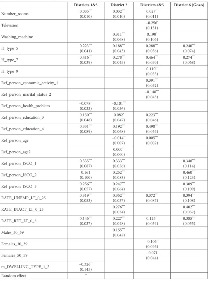
2 3 1var( ) (1 ) . ˆ 1 2 (1 ) ch AB r AB B B B - σ = + + + The variance of 2 η σ is estimated non-paramet-rically, allowing for heteroscedasticity in ech [see Appendix 2, 5]. The two variance components are combined in order to calculate the estimated var-iance-covariance matrix (ˆΣ) of the overall resid-ual of the original model. Once ˆΣ is calculated the original model can be estimated by GLS, the re-sults are in Table 1. In the present analysis, the models for heteroscedasticity have had an R2 around 0.04, so the heteroscedasticity can be con-sidered negligible.
Several models have been estimated for the four areas using variables shared by survey and census plus the aggregated area based variables from the census and just one local level variable in just one area is significant (see Table 1 for the re-gression results).
The consequent stage involves prediction at the household level based on the entire census data and aggregation to small area level. Now, the key assumption is that the models estimated from the survey data apply to census observations.
The parameter estimates obtained from the previous step are applied to the census data so as to simulate the income for each household in the census. A set of 100 simulations has been con-ducted. For each simulation a set of the first stage parameters has been drawn from their corre-sponding distribution simulated at the first stage: the beta coefficients ~β, are drawn from a multi-variate normal distribution with mean ˆβ (the co-efficients of the GLS estimation) and variance-co-variance matrix equal to the one associated to ˆβ. Relating the simulation of the residual terms ˆηc and ech any specific distributional form
assump-tion has been avoided by drawing directly from the estimated residuals: for each cluster the re-sidual drawn is ~ηc and for each household ~ech. The simulated values are based on both the predicted logarithm of income x'ch~β, and on the disturbance terms ~ηc and ~ech using bootstrapped methods:
(
)
ˆ
ln exp T .
ch ch c ch
y = x β + η + e [3] The full set of simulated ˆych is used to calculate
the expected value of each of the poverty meas-ures considered.
For each of the simulated equivalised income distributions a set of small area poverty and in-equality measures has been calculated by aver-aging the simulated equivalised income for each small area and the variance computed over all the 100 simulations gives the standard errors for each small area. As regard to the results, in the next section are reported poverty and inequality meas-ures calculated at the local level for children aged 0–5, 6–13 and 14–17 years.
As usual, in each poverty mapping analysis, we compare figures obtained from the sample sur-vey estimation and from the census for the whole country.
Income figures from the SILC and the census for the whole country show some discrepancies: particularly, the at-risk-of-poverty rate based on SILC is 13.84, the one based on census is 15.33; looking at the average equivalised incomes, the one based on SILC is Lm 3,797, the one based on census is Lm 3,751.
Table 1 Regression results by District: GLS estimates for fixed effects and standard error (in parentheses)
Districts 1&3 District 2 Districts 4&5 District 6 (Gozo)
Number_rooms 0.035(0.010)*** 0.032(0.010)*** (0.011)0.027** Television –0.256(0.151)* Washing_machine 0.311(0.068)*** (0.106)0.190* H_type_5 0.223(0.041)*** 0.188(0.043)*** 0.288(0.056)*** 0.240(0.074)*** H_type_7 0.416(0.039)*** 0.278(0.045)*** 0.464(0.050)*** 0.274(0.068)*** H_type_9 (0.055)0.110** Ref_person_economic_activity_1 0.391(0.052)*** Ref_person_marital_status_2 –0.148(0.043)*** Ref_person_health_problem –0.078(0.033)** –0.101(0.036)*** Ref_person_education_3 0.130(0.048)*** (0.047)0.082* 0.223(0.046)*** Ref_person_education_4 0.331(0.089)*** 0.192(0.068)*** 0.490(0.054)*** Ref_person_age –0.014(0.007)** 0.005(0.002)*** Ref_person_age2 (0.000)0.000** Ref_person_ISCO_1 0.335(0.087)*** 0.333(0.056)*** 0.348(0.114)*** Ref_person_ISCO_2 (0.100)0.161 0.252(0.083)*** 0.460(0.123)*** Ref_person_ISCO_3 0.256(0.057)*** 0.247(0.064)*** 0.309(0.109)*** RATE_UNEMP_LT_0_25 0.319(0.053)*** 0.352(0.057)*** 0.372(0.087)*** 0.394(0.108)*** RATE_INACT_LT_0_25 0.276(0.034)*** 0.402(0.052)*** RATE_RET_LT_0_5 0.146(0.037)*** 0.227(0.048)*** (0.054)0.125** 0.385(0.055)*** Males_50_59 0.155(0.042)*** Females_30_39 –0.106(0.046)** Females_50_59 (0.044)–0.071 m_DWELLING_TYPE_1_2 –0.326(0.145)** Random effect **
The discrepancies can be related to a possi-ble bias which can affect estimators based on pov-erty mapping if there are no area-specific predic-tors to control area specific bias. Demombynes et al. [6] demonstrated that ELL performance de-pends on the locality-level explanatory variables inserted into the income model based on survey data. In our empirical analysis, there was not ex-ternal information to create variable able to incor-porate in the model contextual effect, and unfor-tunately, the variables computed as average clus-ter level on census data are not significant in the specified models. However, in the case of Malta, regional estimates based on direct or small area estimation cannot be computed, and the ELL is the only methodology which could be applied [7]. Being based on a regression model function of a set of diverse type of independent variables, ELL could be seen a sort of multidimensional approach to poverty analysis. Among others, the most im-portant papers describing multidimensional ap-proaches could be Atkinson and Bourguignon [8], Tsui [9], Maasoumi [10], Anand and Sen [11], Sen [12], Duclos, Sahn and Younger [13], Atkinson et al. [14], Atkinson [15], Alkire and Foster [16]; one of the most popular multidimensional approach presented in literature is the one based on fuzzy set theory [17-23].
4. Poverty and inequality measures for children
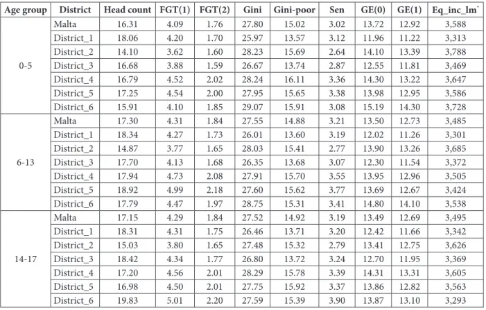
Table 2 reports poverty and inequality meas-ures calculated for the six Districts for children aged 0–5, 6–13 and 14–17 years. Figures 1, 2 and 3 report the percentage of children at-risk-of-pov-erty aged 0–5, 6–13 and 14–17 years among the 68 municipalities. The at-risk-of-poverty rates amongst children increased with increasing age. As an example, the at-risk-of-poverty rate among children within Gozo and Comino increased from 15.9 percent among children aged under 6 to nearly 20 percent within the 14–17 year old age group. This may be explained due to the fact that many households with children aged over 5 tend to have more than one child and less work inten-sity. Consequently, the equivalised income for these households tends to be lower than the other households with a resulting increase in the at-risk-of-poverty rate.
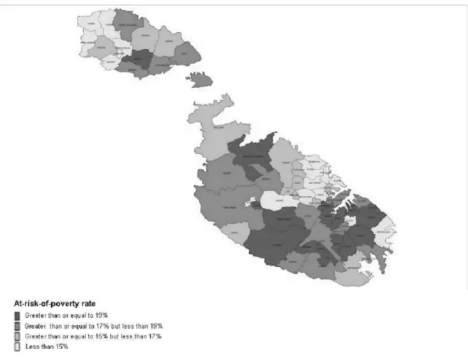
Through this exercise, it is also interesting to observe how the at-risk-of-poverty rates for chil-dren in certain localities differ significantly from that estimated for neighbouring localities. For ex-ample, if we focus on the 0–5 age-group, locali-ties that stand out in particular in this respect are Marsascala in the South Eastern district, Fgura in the Southern Harbour district, Mtarfa and Attard
Table 2 Poverty and inequality indices (%) for children
Age group District Head count FGT(1) FGT(2) Gini Gini-poor Sen GE(0) GE(1) Eq_inc_lm*
0-5 Malta 16.31 4.09 1.76 27.80 15.02 3.02 13.72 12.92 3,588 District_1 18.06 4.20 1.70 25.97 13.57 3.12 11.96 11.22 3,313 District_2 14.10 3.62 1.60 28.23 15.69 2.64 14.10 13.39 3,788 District_3 16.68 3.88 1.59 26.67 13.74 2.87 12.55 11.81 3,469 District_4 16.79 4.52 2.02 28.24 16.11 3.36 14.30 13.22 3,647 District_5 17.25 4.54 2.00 27.95 15.65 3.38 13.98 12.95 3,586 District_6 15.91 4.10 1.85 29.07 15.91 3.08 15.19 14.30 3,728 6-13 Malta 17.30 4.31 1.84 27.55 14.88 3.21 13.50 12.73 3,485 District_1 18.34 4.27 1.73 26.01 13.60 3.19 12.02 11.26 3,301 District_2 14.87 3.77 1.65 28.03 15.41 2.77 13.90 13.26 3,685 District_3 17.70 4.13 1.68 26.35 13.68 3.07 12.30 11.54 3,372 District_4 17.94 4.73 2.08 27.91 15.70 3.55 13.95 12.96 3,505 District_5 18.92 4.99 2.18 27.60 15.62 3.77 13.69 12.67 3,424 District_6 17.79 4.47 1.97 28.75 15.31 3.41 14.80 14.10 3,538 14-17 Malta 17.15 4.29 1.84 27.52 14.92 3.19 13.49 12.69 3,495 District_1 18.31 4.31 1.75 26.46 13.71 3.20 12.42 11.66 3,342 District_2 15.03 3.80 1.65 27.48 15.32 2.79 13.41 12.75 3,626 District_3 18.42 4.34 1.77 26.80 13.72 3.24 12.70 11.95 3,369 District_4 17.20 4.56 2.01 28.29 15.78 3.39 14.31 13.31 3,605 District_5 16.98 4.50 2.01 27.75 15.92 3.37 13.86 12.82 3,563 District_6 19.83 5.01 2.20 27.59 15.39 3.90 13.87 13.10 3,293
Fig. 1. HCR children aged 0–5 by Localities
in the Western district. The at-risk-of-poverty rate for children aged between 0 and 5 was estimated to be less than 15 % in these localities, which is in contrast with neighbouring localities. At the other end of the scale, St. Paul’s Bay in the Northern dis-trict stands out for having a relatively high at-risk-of-poverty rate among young children when com-pared to other localities in the vicinity.
In general, children are considered to be a vul-nerable group. The at-risk-of-poverty rate for per-sons aged between 0 and 17 is, in fact, higher than that estimated for the population as a whole. However when analysing results at locality level, it can be observed that for certain localities the op-posite is true. This is the case in 18 localities for the 0–5 age-group, 10 localities in the 6–13 age group and 6 localities in the 14–17 age groups.
5. Conclusions and recommendations The results derived from this study are of inter-est in their own right, but furthermore they can be applied advantageously within different fields, as will be described below.
From a policy-making point of view, the availa-bility of key indicators at locality level (LAU2) cer-tainly provides a valuable tool in assessing the ef-fectiveness of national strategies and in
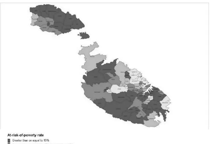
identi-Fig. 3. HCR children aged 14–17 by Localities
fying areas that need to be targeted by new eco-nomic policies, moreover the map representation convey an enormous amount of information about the spread and relative magnitude of pov-erty across localities, in a way which is quickly and intuitively absorbed also by non-technical audiences. Such detailed geographical profiles of poverty and inequality across a country are valu-able inputs for a wide variety of debates and de-liberations, amongst policymakers as well as civil society.
There are also benefits of a technical nature, particularly in terms of sampling strategies for survey studying any economic phenomena that can be derived from this study. Through such an exercise, it is possible to identify economic ho-mogeneity and/or heterogeneity among house-holds in different localities (and potentially in even smaller units within these localities). This is useful when defining strata for stratification sam-pling in any economic survey. For example gener-ally, in stratified sampling, a group of neighbour-ing localities belongneighbour-ing to the same district are grouped into one stratum. However, this study has shown how it may be wise to rethink such strat-ification, since certain localities in the same dis-trict have come across as having very contrasting
realities in terms of economic poverty. Similarly, this study would be useful to determine efficient cluster sampling. The clusters are assumed to be homogeneous such that the sampling variance of the estimators depends on the variation between the clusters and not within them. This study can shed some light on how safe it is to make these assumptions.
One further important advantage of this study is that it can be extended from a national pro-ject into one at the European level. The structures
for this are already in place through the availa-bility of 2011 census data for most countries and the existence of a number of harmonised surveys such as that on Statistics on Income and Living Conditions (EU-SILC), Household Budget Surveys (HBS) and the Labour Force Survey (LFS). As a re-sult, the methods used in this study may be ap-plied to most European countries in order to esti-mate various key economic indicators, thus max-imising the output of these important surveys. References
1. Elbers, C., Lanjouw, J. O. & Lanjouw, P. (2003). Micro-level Estimation of Poverty and Inequality. Econometrica, 71, 335-364. 2. NSO. (2007, July). Census of Population and Housing 2005.
3. NSO. (2006, December). EU-SILC 2005 Final Quality Report.
4. Neri, L., Ballini, F. & Betti, G. (2005). Poverty and inequality mapping in transition countries. Statistics in Transition, 7(1), 135-157.
5. Elbers, C., Lanjouw, J. O. & Lanjouw, P. (2002). Micro-level Estimation of Welfare. Working Paper No 2911. The World Bank, Washington, D.C.
6. Demombynes, G., Lanjouw, J. O., Lanjouw, P. & Elbers, C. (2006). How good a map? Putting Small Area Estimation to the Test. Policy Research Working Paper No. 40155. The World Bank.
7. Betti, G., Gagliardi, F., Lemmi, A. & Verma, V. (2012). Sub-national indicators of poverty and deprivation in Europe: meth-odology and applications. Cambridge Journal of Regions, Economy and Society, 5(1), 149-162.
8. Atkinson, A. B. & Bourguignon, F. (1982). The comparison of multidimensional distributions of economic status. Review of Economic Studies, 49, 183-201.
9. Tsui, K. (1985). Multidimensional generalisation of the relative and absolute inequality indices: the Atkinson-Kolm-Sen approach. Journal of Economic Theory, 67, 251-265.
10. Maasoumi, E. (1986). The measurement and decomposition of multidimensional inequality. Econometrica, 54, 771-779. 11. Anand, S. & Sen, A. K. (1997), Concepts of human development and poverty: a multidimensional perspective. Human Development Papers, United Nations Development Programme (UNDP), New York.
12. Sen, A. K. (1999). Development as freedom. Oxford University Press, Oxford.
13. Duclos, J.-Y., Sahn, D. & Younger, S. D. (2001). Robust multidimensional poverty comparisons. Canada: Université Laval. 14. Atkinson, A. B., Cantillon, B., Marlier, E. & Nolan, B. (2002). Social Indicators: The EU and Social Inclusion. Oxford: Oxford University Press.
15. Atkinson, A. B. (2003). Multidimensional deprivation: contrasting social welfare and counting approaches. Journal of Economic Inequality, 1, 51-65.
16. Alkire, S. & Foster, J. (2011). Counting and multidimensional poverty measurement. Journal of Public Economics, 95(7-8), 476-487.
17. Cerioli, A. & Zani, S. (1990). A fuzzy approach to the measurement of poverty. In: Dagum C. and Zenga M. (Eds). Income and wealth distribution, inequality and poverty. Berlin: Springer Verlag, 272-284.
18. Cheli, B. & Lemmi, A. (1995). A Totally Fuzzy and Relative Approach to the Multidimensional Analysis of Poverty. Economic Notes, 24, 115-134.
19. Cheli, B. & Betti, G. (1999). Fuzzy analysis of poverty dynamics on an Italian pseudo panel, 1985-1994. Metron, 57, 83-104. 20. Betti, G., Cheli, B. & Cambini, R. (2004). A statistical model for the dynamics between two fuzzy states: theory and applica-tion to poverty analysis, Metron, 62(3), 391-411.
21. Belhadj, B. (2011). A new fuzzy unidimensional poverty index from an information theory perspective. Empirical Economics, 40(3), 687-704.
22. Belhadj, B. (2012). New weighting scheme for the dimensions in multidimensional poverty indices. Economic Letters, 116(3), 304-307.
23. Belhadj, B. & Limam, M. (2012). Unidimensional and multidimensional fuzzy poverty measures: New approach. Economic Modelling, 29(4), 995-1002.
Authors
Gianni Betti — PhD in Applied Statistic, Associate Professor, Department of Statistics and Economics, University of Siena (7,
Piazza S. Francesco, Siena, 53100, Italy; e-mail: [email protected]).
Etienne Caruana — MSc in Statistics & Operations Research, Director of Social Statistics, National Statistics Office (Lascaris,
Valletta VLT 2000, Malta; e-mail: [email protected]).
Sarah Gusman — MSc in Statistics, Principal Statistician, National Statistics Office (Lascaris, Valletta, Malta; e-mail: gusman.
Laura Neri — PhD in Applied Statistic, Assistant Professor in Statistics and Economics, Department of Economics and