Number 28 -2015
RATIO MATHEMATICA
Journal of Foundations
and Applications of Mathematics
Managing editors:
Sarka Hoskova-Mayerova,
Fabrizio Maturo
Editorial Board
R. Ameri, Teheran, Iran A. Beutelspacher, Giessen, Germany A. Ciprian, Iasi, Romania P. Corsini, Udine, Italy
I. Cristea, Nova Gorica, Slovenia F. De Luca, Pescara, Italy S. Cruz Rambaud, Almeria, Spain B. Kishan Dass, Delhi, India J. Kacprzyk, Warsaw, Poland C. Mari, Pescara, Italy S. Migliori, Pescara, Italy F. Paolone, Napoli, Italy I. Rosenberg, Montreal, Canada M. Scafati, Roma, Italy M. Squillante, Benevento, Italy L. Tallini, Teramo, Italy I. Tofan, Iasi, Romania A.G.S. Ventre, Napoli, Italy T. Vougiouklis, Alexandroupolis, Greece R. R. Yager, New York, U.S.A.
Publisher
A.P.A.V.
Accademia Piceno – Aprutina dei Velati in Teramo
Honorary editor
Franco Eugeni
Editor in chief
15
Approach of the value of an annuity when
non-central moments of the capitalization
factor are known: an R application with
interest rates following normal and beta
distributions
Salvador Cruz Rambaud
1, Fabrizio Maturo
2, Ana María Sánchez
Pérez
31Department of Economics and Business, University of Almería, Spain,
2Department of Management and Business Administration, University of
Chieti-Pescara, Italy, [email protected]
3Department of Economics and Business, University of Almería, Spain,
(The authors are entered in alphabetical order by their last name)
Abstract
This paper proposes an expression of the value of an annuity with payments of 1 unit each when the interest rate is random. In order to attain this objective, we proceed on the assumption that the non-central moments of the capitalization factor are known. Specifically, to calculate the value of these annuities, we propose two different expressions. First, we suppose that the random interest rate is normally distributed; then, we assume that it follows the beta distribution. A practical application of these two methodologies is also implemented using the R statistical software.
Keywords: annuity; random interest rate; non-central moments.
2010 AMS subject classification: 91G30; 46N30; 65C60; 91G70; 62P05. doi: 10.23755/rm.v28i1.25
16
1 Introduction
This study aims to determine an approximate expression for the present, or final, value of an annuity when the interest rate is random. In the context of annuities assessment, the interest rate has a great relevance because even small changes may cause major changes in the total annuity value. Thus, the determination of the value of the interest rate should be carried out as accurately as possible.
The traditional approach treats interest rates deterministically; indeed, in contexts of certainty, the use of a single possible value for each period may be enough [8]. However, for those operations developed in uncertain environments, it is more reasonable the formulation of potential scenarios, which are subsequently reduced to one by statistical treatment [2].
The determination of the interest rate value must be based on the current situation, as well as on its possible future evolution, of both companies and environment. In this way, if prospects are unfavorable, interest rates must be higher, compared to more favorable situations, and hence to reduce the operation value as a consequence of the risk attached to it. However, in most cases, determining the interest rate of a financial operation is subject to the propensity/aversion to risk of the agent to be responsible for the assessment. In this sense, the adopted interest rate would be affected by a degree of subjectivity that may over/undervalue the project [7].
In this paper, we consider the interest rate as a random variable that is represented as X. Therefore, the capitalization factor,
1
i
, is also a random variable represented as U. Obviously, it is verified thatU
1
X
, thus, the relationship between the mean and standard deviation of both variables is as follows:As a result, if X is defined in an interval [ ba, ], then U will be in the interval ]
1 , 1
[a b . Henceforth, when the mean and standard deviation are mentioned we will refer, unless otherwise specified, to the random variable U.
In this case, the final value of an n-payment annuity, with payments of 1 unit each made at the end of every year (annuity-immediate), valued at the rate
X, would be the following random variable:
Thus, its expected value is: X U 1 and
U
X. 1 2 1 1 n U n U U U s . (1)17
On the other hand, the final expected value of an n-payment annuity, with payments of 1 unit each made at the beginning of every year (annuity-due), valued at the rate X, would be:
being
(
r)
r
E
U
the moment of order r, with respect to the origin, of the random variable U; hence, if the random variable is discrete, it adopts the following expression [1]:being pi the probability that the random variable takes the value ui. In the
continuous case, the expression of the moment of order r is:
for all values of r, being f(u) the density function of the random variable U.
As indicated, this paper proposes a mathematical expression of the final value of an annuity, immediate or due; specifically, we compute it using a random interest rate and suppose that the non-central moments of the capitalization factor are known. Section 2 shows the case of interest rates following the normal distribution. Section 3 takes into account the beta distribution, as an example of distribution with finite range. Section 4 shows a practical application using the R statistical software. Lastly, the conclusions are presented.
2 The expression of the final value of an annuity
when the interest rate follows a normal
distribution
The successive non-central moments of order r, with respect to the normal distribution, can be computed according to its mean and variance2
[4]: . 1 ) ( ) ( ) ( ) 1 ( ) ( 1 2 1 2 1 n n U n E E U E U E U s E , ) ( ) ( ) ( ) ( 2 2 1 n n U n E U E U E U s E (2)
k i r i i r r EU pu 1 ) ( , (3)
max min d ) ( ) ( u u r r E U uf u u , (4)18 0 1;
1
; 2 2 2
; 3 2 3 3 ; 4 2 2 4 4
6
3
; 5 3 2 4 5 10 15 ; 6 4 2 2 4 6 6
15
45
15
; 7 5 2 3 4 6 7
21
105
105
; 8 6 2 4 4 2 6 8 8 28 210 420 105 . Therefore, the final value of an n-payment annuity, with payments of 1 unit each made at the end of every year (annuity-immediate) that is the sum of the n first non-central moments
1 0 n r r
, is composed of the following partial sums:
. 1 1 1 1 0 1 2
n n r r n This can be written as
1 0 0 0 n r r r . . 2 ) 28 21 15 10 6 3 1 ( 1 2 2 2 6 5 4 3 2 2
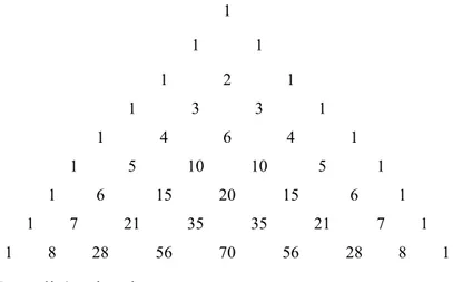
n r r r The coefficients of successive powers of , in parentheses, are the numbers in red in the following Tartaglia’s triangle (Figure 1):
Figure 1: Tartaglia’s triangle.
1 1 1 1 2 1 1 3 3 1 1 4 6 4 1 1 5 10 10 5 1 1 6 15 20 15 6 1 1 7 21 35 35 21 7 1 1 8 28 56 70 56 28 8 1
19 . 4 3 ) 70 35 15 5 1 ( 3 1 4 4 4 4 3 2 4
n r r r The coefficients of successive powers of , enclosed in the parentheses, are the numbers in green of the previous Tartaglia’s triangle.
, 6 15 ) 28 7 1 ( 15 1 6 6 6 2 6
n r r r whose coefficients are in blue.
And so forth.
In short, the sum of the n first non-central moments is:
E(( 1)/2) 1 1 2 2 2 1 0 2 ) 1 2 ( 5 3 1 1 1 n k n k r k r k n n r r k r k ,which can also be written as follows:
. 2 )! 1 ( 2 )! 1 2 ( 1 1 E(( 1)/2) 1 1 2 2 2 1 1 0
n k n k r k r k k n n r r k r k k (5)This method is used to calculate the final value of an n-payment annuity, with payments of 1 unit each made at the end of every year (annuity-immediate), with a random interest rate. Whereas, the calculation of the final value of an n-payment annuity, with payments of 1 unit each made at the beginning of every year (annuity-due), has the following expression:
. 2 ) 1 2 ( 5 3 1 1 1 E( /2) 1 2 2 2 1
n k n k r k r k n n r r k r k (6) In equations (5) and (6), the function E x( ) represents the integer part of x.To carry out the calculations in a comfortable and orderly manner, we propose to refer to Table 1.
20
3 The expression of the final value of an annuity
when the interest rate follows a beta
distribution
The best known random variable with a bounded range is the beta distribution. The expression of the non-central moments of the standard beta distribution of parameters
and is the following (rN ) [3]:. ) 1 ( ) 1 )( ( ) 1 ( ) 1 ( ) ( ) ( ) ( ) ( r r r r r (7) In this case, it is not feasible to give a closed expression of the sum of the n first non-central moments, but, having in mind that(1)(), we can
write the following recurrence relation [5]:
r r r r 1 . (8)
Tartaglia’s triangle Exponents of
0 1 2 3 4 1 0 - - - - 1 1
1 - - - - 1 2 1
2
0 - - - 1 3 3 1 3
1 - - - 1 4 6 4 1 4 2 0 - - 1 5 10 10 5 1
5
3
1 - - 1 6 15 20 15 6 1
6
4
2
0 - 1 7 21 35 35 21 7 1 7 5 3
1 - 1 8 28 56 70 56 28 8 1 8 6 4 2 0 0 2 4 6 8 1 1 3 15 105 21
Table 1. Tabular organization for calculations (the number that occupies the place ( sr, ) in Tartaglia’s triangle is equal to the sum of those in places
) 1 , 1
(r s and (r1,s).
However, it should be considered that the above mentioned moments refer to the standard beta distribution, Z, of parameters,
and , that is, with range]. 1 , 0
[ Furthermore, to obtain the moments
r
corresponding to the distributionU without normalize, that is to say, the beta distribution of parameters and , with range [a,b]: , ) (b a Z a U (9)
it is necessary to consider the relationship between its moment-generating functions [6]: ). ) (( e ) ( ) (t M ( ) t M b a t M at Z Z a b a U (10) Therefore, having in mind the expression of the nth derivative of a product of functions, we can write:
. ) ) (( ) ( e ) ) (( d d e d d ) ( d d 0 ) 0
r k k r Z k r at k r k Z k r k r at k k U r r t a b M a b a k r t a b M t t k r t M t Therefore,
r k k r k r k t U r r r a b a k r t M t 0 0 ) ( ) ( d d . (11)4 Calculation of the value of an annuity, with
payments of 1 unit each: an R application
Next, we are going to obtain the final value of an annuity, with payments of 1 unit each for five years through the different expressions developed in this work. In its calculus we consider that the payments are made at the end, or the
22
beginning, of each period. Present value calculation has been omitted provided it can be carried out similarly.
Given that in this work it has been contemplate that non-central moments of the capitalization factor are known, two possible options have been considered, where discount rate, X, follows:
a normal distribution;
a beta distribution.
Discount rate with a normal distribution
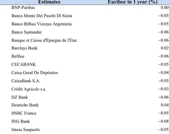
To estimate the mean and variance of the normal distribution, we consider Euribor’s data containing the estimated annual Euribor of different banks (Table 2), available at http://www.emmi-benchmarks.eu/euribor-org/euribor-rates.html. Specifically, the Euribor at 12 months is considered on 27/07/2016.
Estimates Euribor in 1 year (%)
BNP-Paribas 0.00
Banca Monte Dei Paschi Di Siena 0.05 Banco Bilbao Vizcaya Argentaria 0.05
Banco Santander 0.06
Banque et Caisse d'Épargne de l'État 0.06
Barclays Bank 0.02
Belfius 0.06
CECABANK 0.05
Caixa Geral De Depósitos 0.04
CaixaBank S.A. 0.05
Crédit Agricole s.a. 0.03
DZ Bank 0.06
Deutsche Bank 0.04
HSBC France 0.05
ING Bank 0.08
Intesa Sanpaolo 0.05
Table 2: Euribor distribution at 27/07/2016.
Source: http://www.emmi-benchmarks.eu/euribor-org/euribor-rates.html. To enter the data in the R environment, it is necessary to create a vector as follows:
23
>data=c(0.00,-0.05,-0.05,-0.06,-0.06,0.02,-0.06,-0.05,-0.04,-0.05,-0.03,-0.06,0.04,-0.05,-0.08,-0.05,-0.12,-0.03,-0.05,-0.04,-0.06)
To check for normality of the data, we need the R package “tseries”; thus, the Jarque-Bera Test is implemented:
> library(tseries) > jarque.bera.test(data)
We can accept the normality of the data because the p-value is greater than 0.05 (X-squared = 3.559, df = 2, p-value = 0.1687).
Following a preliminary analysis, we obtain 0.0442 and
0.0332
using the following scripts:
> mean(data) > sd(data)
The expressions formulated in Section 2 allow computing the expected final value when the expression of the non-central moments of the capitalization factor is known.
Now, we suppose to compute the final value of an annuity, with payments of 1 unit each for five years using the estimated mean and variance. Thus, if the payments of the annuity are at the end of each period, the final value is:
4.958541. 4 0
r r It is possible to check this result building a function to compute the sum of the non-central moments of the normal distribution for annuities whose payments are at the end of each period, with a duration of k years (however, firstly, we need to load the “moments” library):
>library(moments)
>sum_k_moments_post=function(data,k){ app.moments_post=rep(NA,k)
for (i in 0:(k-1)) app.moments_post[i+1]=moment(data, central = FALSE, absolute = FALSE, order =i)
sum_moments_post=sum(app.moments_post)+(k-1) return(sum_moments_post) }
24
Instead, in case the final value of an annuity, with payments of 1 unit each at the beginning of every year, for five years, we obtain:
4.958539. 5 1
r r Also in this case, we can check the result by creating a function to compute the sum of the non-central moments of the normal distribution for annuities whose payments are at the beginning of each period, with a duration of k years:
> sum_k_moments_ant=function(data,k){ app.moments_ant=rep(NA,k)
for (i in 1:k) app.moments_ant[i]=moment(data, central = FALSE, absolute = FALSE, order =i)
sum_moments_ant=sum(app.moments_ant)+k return(sum_moments_ant) }
>sum_k_moments_ant(data,5)
Using the formulation proposed in equation 5 (annuities with payments at the end of each period) and equation 6 (annuities with payments at the beginning of each period), we reach the same results (replacing the values of the mean and the standard deviation, it is simple to demonstrate this identity).
Discount rate with a beta distribution
Because the beta distribution is suitable to approximate also the data of Table 2, we refer to the same data of Euribor with the aim to compare it with the results obtained in the previous paragraph.
At this purpose we load the data of Table 2 and the R packages “actuar” and “EnvStats” as follows:
>library(actuar) >library(EnvStats)
Then, we create a function to normalize data and we apply it to the data of Table 2 as follows:
>nor=function(x){(x-min(x))/(max(x)-min(x))} >data2=nor(data)
Afterwards, we estimate the shapes of the beta distribution with the function “ebeta”:
25
Following this approach, we get the shapes parameters a = 2.394501 and b
= 2.66557. Then, we build a function to compute the mean and the standard
deviation: >mean_beta=function(a,b){a/(a+b)} >mean_beta(2.394501,2.665577) 0.4732142 >var_beta=function(a,b){a*b/((a+b)^2*(a+b+1))} >var_beta(2.394501,2.665577) 0.0411352
As known, a generic moment of the standard beta distribution is given by:
( ) ( ) r r r (12) where ()r (1)(r1).
To compute the moments of the standard beta distribution using this method, we need a function to calculate the factorial:
>fattoriale_crescente=function(n,f){n*factorial(x=n+f-1)/factorial(x=n)}
In this way, we can compute the moments as:
>momento_beta=function(a,b,f){fattoriale_crescente(a,f)/fattoriale_cresce nte((a+b),f)}
where a and b are the shapes parameters and f represents the order of the moment.
Using these codes, it is simple to calculate the sum of the moments of the standard beta distribution. However, we need the non-central moments of the original beta distribution (without normalize). At this purpose, we build a function to perform Equation (11) and obtain the non-central moments of the original beta distribution.
We set a as the lower bound of our interest rates, b as the upper bound of our interest rates, c and d as the parameters of the standard beta distribution, n as the number of years:
>c=2.394501 >d=2.665577
26 >a=-0.12 >b=0.04 >n=5 >momento_nn_normalizzato=function(n,a,b,c,d){for(k in 0:n) { m=mbeta(n-k, c, d) moment_nn_norm=sum( choose(n,k)*(a^k)*((b-a)^(n-k))*m )} return(moment_nn_norm)}
Afterwards, we present two functions: the first one computes the final value of an n-payment annuity, with payments of 1 unit each made at the end of every year (annuity-immediate); the second one calculates the final value of an n-payment annuity, with n-payments of 1 unit each made at the beginning of every year (annuity-due).
The first function is built as follows:
>sum_n_moments_non_norm_beta_pag_anticip=function(n,a,b,c,d){ app=rep(NA,n)
for (i in 1:n) app[i]=(momento_nn_normalizzato(i,a,b,c,d)+1) return(sum(app))}
>sum_n_moments_non_norm_beta_pag_anticip(5,a,b,c,d)
Thus, the final value of an n-payment annuity, with payments of 1 unit each made at the end of every year (annuity-immediate) for five years is:
5 1 4.892854 r r
.The second function is provided by the following code:
>sum_n_moments_non_norm_beta_pag_post=function(n,a,b,c,d){ app2=rep(NA,n) for (i in 0:(n-1)) app2[i+1]=momento_nn_normalizzato(i,a,b,c,d) app2[2:n]=app2[2:n]+1 return(sum(app2))} >sum_n_moments_non_norm_beta_pag_post(5,a,b,c,d)
Therefore, with our data, the final value of an n-payment annuity, with payments of 1 unit each made at the beginning of every year (annuity-immediate) for five years is:
4 0 4.892879 r r
.27
5 Conclusions
In this paper we have presented two methodologies to obtain the value of an annuity whose discount rate is a variable known in terms of random. Once the expected value of the discount rate has been analyzed through the non-central moments of the discount factor, the expression for determining the expected final value of an n-payment annuity has been deduced.
Specifically, the theoretical development of this methodology has been carried out in two different ways: by supposing that the interest rate follows a normal distribution, and considering that it follows a beta distribution.
Furthermore, we provided the code to reproduce our results with the R statistical software (available in Appendix 1).
Our results show slight differences between the estimates of the same data, approximating these with different distributions. This shows how the choice of the distribution of the approximation of data is important for the calculation of the value of an annuity when interest rates are represented by random variables.
28
Appendix 1: Replication material
data=c(0.00,-0.05,-0.05,-0.06,-0.06,0.02,-0.06,-0.05,-0.04,-0.05,-0.03,-0.06,0.04,-0.05,-0.08,-0.05,-0.12,-0.03,-0.05,-0.04,-0.06) library(tseries) jarque.bera.test(data) mean(data) sd(data) library(moments) sum_k_moments_post=function(data,k){ app.moments_post=rep(NA,k)
for (i in 0:(k-1)) app.moments_post[i+1]=moment(data, central = FALSE, absolute = FALSE, order =i)
sum_moments_post=sum(app.moments_post)+(k-1) return(sum_moments_post)}
sum_k_moments_post(data,5)
sum_k_moments_ant=function(data,k){ app.moments_ant=rep(NA,k)
for (i in 1:k) app.moments_ant[i]=moment(data, central = FALSE, absolute = FALSE, order =i)
sum_moments_ant=sum(app.moments_ant)+k return(sum_moments_ant)} sum_k_moments_ant(data,5) library(actuar) library(EnvStats) nor=function(x){(x-min(x))/(max(x)-min(x))} data2=nor(data)
ebeta(data2, method = "mle") mean_beta=function(a,b){a/(a+b)} mean_beta(2.394501,2.665577)
29 var_beta=function(a,b){a*b/((a+b)^2*(a+b+1))} var_beta(2.394501,2.665577) fattoriale_crescente=function(n,f){n*factorial(x=n+f-1)/factorial(x=n)} momento_beta=function(a,b,f){fattoriale_crescente(a,f)/fattoriale_crescente ((a+b),f)} momento_nn_normalizzato=function(n,a,b,c,d){ for(k in 0:n) { m=mbeta(n-k, c, d) moment_nn_norm=sum( choose(n,k)*(a^k)*((b-a)^(n-k))*m ) } return(moment_nn_norm)} sum_n_moments_non_norm_beta_pag_anticip=function(n,a,b,c,d){app=rep (NA,n) for (i in 1:n) app[i]=(momento_nn_normalizzato(i,a,b,c,d)+1) return(sum(app))} sum_n_moments_non_norm_beta_pag_anticip(5,a,b,c,d) sum_n_moments_non_norm_beta_pag_post=function(n,a,b,c,d){ app2=rep(NA,n) for (i in 0:(n-1)) app2[i+1]=momento_nn_normalizzato(i,a,b,c,d) app2[2:n]=app2[2:n]+1 return(sum(app2))} sum_n_moments_non_norm_beta_pag_post(5,a,b,c,d)
30
Bibliography
[1] Calot, G. (1974). Curso de estadística descriptiva. Madrid: Ed. Paraninfo. [2] Cruz Rambaud, S. and Valls Martínez, M.C. (2002). “La determinación de la tasa de actualización para la valoración de empresas”. Análisis Financiero, 87, 72-85.
[3] Fisz, M. (1963). Probability theory and mathematical statistics, 3rd Edition. New York: John Wiley and Sons, Inc.
[4] Mood, A.M.; Graybill, F.A. and Boes, D.C. (1974). Introduction to the theory of statistics, 3rd Edition. New York: McGraw Hill.
[5] Rice, J.A. (1995). Mathematical statistics and data analysis (2nd Ed.). California: Ed. Duxbury Press.
[6] Spiegel, M.R. (1975). Probability and Statistics. United States of America: Ed. McGraw-Hill.
[7] Suárez Suárez, A.S. (2005). Decisiones óptimas de inversión y financiación en la empresa. Madrid: Ed. Pirámide.
[8] Villalón, J.G.; Martínez Barbeito, J. and Seijas Macías, J.A. (2009). “Sobre la evolución de los tantos de interés”. XVII Jornadas de Asepuma y V Encuentro Internacional, 17, 1, 502.