A Model to Simulate Multimodality in a Mesoscopic Dynamic Network Loading Framework

(1)

Research Article

A Model to Simulate Multimodality in a Mesoscopic Dynamic

Network Loading Framework

Massimo Di Gangi and Antonio Polimeni

Dipartimento di Ingegneria, Universit`a degli Studi di Messina, C.da di Dio S. Agata, 98166 Messina, Italy Correspondence should be addressed to Massimo Di Gangi; mdigangi@unime.it

Received 25 July 2016; Accepted 13 October 2016; Published 11 January 2017 Academic Editor: Zhi-Chun Li

Copyright © 2017 M. Di Gangi and A. Polimeni. This is an open access article distributed under the Creative Commons Attribution License, which permits unrestricted use, distribution, and reproduction in any medium, provided the original work is properly cited. A dynamic network loading (DNL) model using a mesoscopic approach is proposed to simulate a multimodal transport network considering en-route change of the transport modes. The classic mesoscopic approach, where packets of users belonging to the same mode move following a path, is modified to take into account multiple modes interacting with each other, simultaneously and on the same multimodal network. In particular, to simulate modal change, functional aspects of multimodal arcs have been developed; those arcs are properly located on the network where modal change occurs and users are packed (or unpacked) in a new modal resource that moves up to destination or to another multimodal arc. A test on a simple network reproducing a real situation is performed in order to show model peculiarities; some indicators, used to describe performances of the considered transport system, are shown.

1. Introduction

In a multimodal transport system, users can organize their journey by considering the available transport features, with the aim to minimize their perceived cost. Therefore, it is important to have the opportunity to explicitly simulate the change among the available transport modes.

This paper discusses a dynamic network loading (DNL) model for the simulation of a multimodal transport system through a mesoscopic approach. The mesoscopic approach allows the evaluation of some traffic indicators (as flows, den-sity, and queues) grouping the vehicles into packets made up, in general, by several users having homogenous characteris-tics (i.e., path followed, departure time, and speed).

Multimodal features within DNL have been here mod-elled by introducing some original extensions to mesoscopic modelling for a more realistic representation of the opera-tions occurring in a transportation system; in particular they concern the following:

(i) the ability to take into account the physical occupa-tion of vehicles in the queue;

(ii) the articulation of users into classes and the man-agement of the FIFO discipline in the case of users belonging to different classes;

(iii) the ability to manage, at the same time and on the same network, different modes of transport and to simulate operations related to the change, en-route, among available modes.

The paper is structured as follows: after a concise lit-erature review reported in Section 2, in Section 3, after an illustration of the proposed simulation model (considering the representation of demand and supply and the definition of the loading model), the approach followed to simulate different modes on the same network, considering the aggregation and the unpacking of the modal resources, is described. An application to a test network of the pro-posed model and some comments on obtained results are shown in Section 4. Finally, some conclusions and perspec-tives for further planned deepening are briefly outlined in Section 5.

2. Literature Review

In this section, a concise literature review related to the main aspects of the paper is provided: the simulation of multi-modal transport systems and the dynamic network load-ing.

Volume 2017, Article ID 8436821, 16 pages https://doi.org/10.1155/2017/8436821

(2)

2.1. Background on Multimodal Transport. Various aspects are involved in modelling a multimodal transport system such as network representation, users’ behaviour, users’ perception, and preferences.

In order to formulate the problem, many ways to rep-resent the multimodal network were formulated such as a hypergraph (space-time graph) representation [1], a hierar-chical graph approach [2], and an expanded graph approach [3]. In this context, the shortest path evaluation between origin and destination can be performed using either a specific algorithm, like Dijkstra algorithm [4], or others [1, 5, 6]. Ambrosino and Sciomachen [7] propose an algorithm to find the shortest path in a multimodal network optimizing the performances of the modal change.

In dell’Olio et al. [8] a stated preferences survey was designed to explore the willingness to pay by users, consider-ing the transfer time in the multimodal systems, the available services, and the information provided. Similarly, in Arentze and Molin [9] the stated preferences surveyed data was used to calibrate a travel choice model in a multimodal network. Another aspect in a multimodal transport systems is related to the demand management, for example, introducing charges (i.e., parking, access to restricted areas) or varying transit fares to address the users to a specific transport mode and stimulate the modal split. Wu et al. [10] developed a strategy to define toll and fares with the aim to evaluate the impacts of different policies to reduce congestion. In Shi and Li [11] the effect of simultaneous modification of parking charge and transit fare, assuming the demand elastic, was analyzed. Daganzo [12] evaluated the transit fares and the tolls can address the system towards the system optimum.

The user perception is an investigated field in transport simulation, despite being in specific topics [13, 14]. Modesti and Sciomachen [15] proposed an utility function in a mul-timodal network (car, transit, and pedestrian) considering arc costs, arc travel times, and also the users’ preferences in transportation modalities.

In Spickermann et al. [16] some possible development scenarios for a city that adopts a multimodal transport system were analyzed. Kramers [17] investigated some information systems for multimodal and public transport users with the goal to identify the users’ requirements to be satisfied by the information system. Diana [18] evaluated the modal diversion of the users considering habits, cognitive, and affec-tive attitudes. Furthermore, user’s satisfaction [19] can be measured in a multimodal system (in the case of public transport), considering a set of attributes (such as punctuality, cleaning, comfort, and cost).

2.2. Background on Dynamic Network Loading. Considering the traffic assignment field, several formulations were pro-posed in literature to tackle the problem.

In static approach, Cantarella [20] proposed a fixed-point formulation in a multimodal network with elastic demand, considering different classes of users. Fernandez et al. [21] proposed some models to formulate network equilibrium with combined modes, modelling the network as the combi-nation of different subnetworks (one for each transport mode

considered). An equilibrium model in a multimodal network was proposed by Garc´ıa and Mar´ın [22] considering explicitly users’ behaviour in the mode choice/switch. Liu and Meng [23] proposed an user equilibrium with elastic demand to model users’ behaviour considering the interactions between cars and buses flows. Concerning dynamic approach, Bajwa et al. [24] adopted a dynamic traffic simulation model, with a mesoscopic representation of flows, to simulate a multimodal system able to model the choices related to departure time, mode, and route. Using a dynamic approaches it is necessary to evaluate how the user flow is loaded on the arcs of the network, defining a dynamic network loading (DNL) as a component of the Dynamic Traffic Assignment (DTA) [25]. In general, DNL includes a delay model (i.e., [26]) and an exit model (i.e., [27]) and gives as outputs some network indicators (flows, travel times, queues, etc.).

A DNL model is able to simulate the flow propagation in dynamic assignment providing some network indicators. The approaches to solve the problem can be classified considering the function on which they are based (exit function or link travel time [28–30]) or considering the aggregation level of the assignment model (macroscopic, i.e., [31]; mesoscopic, i.e., [32]; microscopic, i.e., [33]). Relating to the link travel time function, various expressions are proposed in literature ranging from linear functions [30] to polynomial functions [34].

Considering the exit function the works of Daganzo [35] and Smith [36] and the study conducted by Mahmassani et al. [37] can be cited.

Assumptions adopted on evolution of queues can also be used as a method to categorize the DNL models [38]; following this way models can be distinguished between link based and node based. The former [39, 40] are focused on link cost functions; the latter [35, 41, 42] consider flow splitting at nodes.

Concerning the mesoscopic approach, S´anchez-Rico et al. [43] propose to solve DNL with a discrete event algorithm based on flow discretization. Celikoglu and Dell’Orco [40] propose a solution algorithm implementing an exit func-tion with respect to capacity constraints and considering acceleration and deceleration on the packets. Linares et al. [44] present a multiclass DNL with a continuous link based approach with discrete demand.

3. Multimodal Transport Simulation Model

In the following of this paragraph the proposed approach to simulate a multimodal transport network considering en-route change of the transport modes is shown. It is based on development of a model previously presented by one of the authors [45]; however, to make the subject more understandable to the reader, some concepts already defined are replicated. The proposed improvements are highlighted by specifying explicitly the differences with the original model.

3.1. General Description. In this approach, simulations are

(3)

S

Running Queuing

m n

La

xSa La− xSa

Figure 1: Schematic representation of an arc.

of simplicity (but without prejudice to the generality of the

treatment), of constant amplitudeΔ𝑡, indicating with 𝜏 the

current time within the time interval,𝜏 ∈ [0, Δ𝑡]. Following

these definitions, the absolute time𝑡 can be evaluated as 𝑡 =

(𝑇 − 1) ⋅ Δ𝑡 + 𝜏.

The transportation network is represented conventionally

by means of a graph(𝑁, 𝐴), where 𝑁 is the set of nodes and

𝐴 is the set of arcs.

Outflow conditions are considered homogeneous on each arc and constant for the entire duration of an interval. They are estimated at the beginning of each interval and considered valid for the entire duration of the interval. This assumption also allows that the results are independent of the order in which the packets are moved. Once outflow characteristics (of arcs) for an interval are known, it is possible to track the movements of vehicles on each arc depending on the assumptions on the model of arc and movement rules defined below.

To define the performance associated with arc 𝑎 ∈ 𝐴

between nodes 𝑚 and 𝑛 ∈ 𝑁, whose length is indicated

by 𝐿_𝑎, the arc is divided into two segments by a section

𝑆 whose position, 𝑥𝑆

𝑎, can assume values between 0 and

𝐿_𝑎, as shown in Figure 1. In the absence of queue, at the

generic time𝜏, the value of the abscissa 𝑥𝑆_𝑎 is equal to𝐿_𝑎.

The part of the arc with𝑥 ∈ [0, 𝑥𝑆_𝑎[ is defined as running

segment, while the remaining part, with 𝑥 ∈ [𝑥𝑆_𝑎, 𝑙_𝑎], is defined as queuing segment. The calculation of the value of

𝑥𝑆

𝑎, that is the position taken by the section𝑆, is conducted

at the beginning of each interval and depends on the outflow conditions on the arc defined by the loading model. In particular, in Section 3.3.1, it is shown how this value is related with the packets movements and the queue on the arc.

3.2. Demand Model. Due to the available computing power, in current practice mesoscopic models using packet approach usually consider packets consisting of a single unit. There-fore, it seems appropriate to update the terminology used commonly in the description of the operations performed to simulate a transportation system using a mesoscopic modelling approach. For this purpose, an essential dictionary explaining the meaning of the terminology used in the remainder of the discussion is introduced.

User. It is basic unit that uses the transportation system to move between an origin and a destination. The user term may be referred to passengers travelling on the network or may be extended by analogy to the freight transport by substituting loading units (pallet and container) in place of the passen-gers.

Modal Unit. It is service, equipment, or vehicle of transport mode used by the user to perform a part or the whole trip between origin and destination. Each modal unit is defined by the mode of transport that represents and a class that specifies its dimensional and performance characteris-tics.

Point. It is entity, placed on the graph of the transport network, that represents a modal unit moving on the network. Demand is described in terms of users travelling on the network using a modal unit; modal units having the same characteristics are grouped into a single class. Each class of modal unit is characterized by the values of some coefficients that define the characteristics in terms of speed, occupancy, and capacity to receive users [45].

In the proposed model, the concept of path followed by an user is generalized. As a matter of fact, some modal units can have a predetermined route (i.e., an urban transit line, a ferry service, and a container shipping line) and the user can choose the whole (of a part) of this route to define its path to reach destination. The followed path can thus be then defined, in general, between two nodes of the network (not necessarily the origin and destination of the trip).

Let𝐾(𝑟𝑠, 𝑢) be the set of paths connecting node 𝑟 with

node𝑠 and followed by modal unit of class 𝑢 and Ω_𝑟𝑠 the

directed acyclic subgraph (of the graph of the network 𝐺)

made up by the arcs belonging to the set of paths𝐾(𝑟𝑠, 𝑢).

A modal unit belonging to class𝑢 leaving at time instant 𝑡

and moving on the subgraphΩ_𝑟𝑠is described through a point

𝑃 ≡ {𝑡, Ω_𝑟𝑠, 𝑢} that is, for calculation, a punctual entity that

moves on the network.

3.3. Dynamic Network Loading Model. In this section the dynamic network loading model is described, considering both the movement rules of points within each arc seg-ment and how the choice of the next arc is conducted. It should be noted that the possibility of simulating these operations consistent with the degree of approximation inherent in a mesoscopic approach is described here; a more detailed simulation requires the use of microscopic models.

3.3.1. Packets Movements. At time𝜏 of interval 𝑇, let 𝑃 ≡

{𝑡, Ω_𝑚𝑠, 𝑢} be a point left at time 𝑡 (where 𝑡 < (𝑇−1)⋅Δ𝑡+𝜏) that

has not yet reached its destination; its position on the graph

is represented by a point located at abscissa𝑥 of arc 𝑎(𝑚, 𝑛)

belonging to subgraphΩ_𝑚𝑠.

Let V_𝑎𝑇 be the speed on running segment of this arc

during the interval𝑇, 𝑘_𝑎maxthe maximum density on the arc,

and𝑄_𝑎the capacity of the final section of the arc (eventually

depending on 𝑇) such that 1/𝑄_𝑎 is the average service

(4)

The value of𝑥𝑆_𝑎is within the interval[0, 𝐿_𝑎] and depends on outflow conditions of the arc. It is determined at the beginning of each evaluation interval on the basis of the number of vehicles making up the queue and the charac-teristics of the class (occupancy parameter that indicates the space occupied by a single facility of the class) they belong [45].

Recalling thatΔ𝑡 is the time length of an interval and 𝜏 ∈

[0, Δ𝑡], with reference to the arc model described before, the following cases may occur:

(i) if 𝑥 < 𝑥𝑆_𝑎 the (representative point of) packet 𝑃

is located on the running segment, it moves at a

speed V_𝑎𝑇 and, within the interval𝑇, it may reach

a maximum abscissa𝑥𝑆_𝑎; consequently the distance

that can be covered on the segment is given by

min{𝑥𝑆

𝑎 − 𝑥, (Δ𝑡 − 𝜏) ⋅ V𝑎𝑇}. If it happens that 𝑥𝑆𝑎−

𝑥 < (Δ𝑡 − 𝜏) ⋅ V_𝑎𝑇_{, the packet}_{𝑃 enters the queuing}

segment of arc𝑎, before the end of the interval, at time

𝜏󸀠 _{= 𝜏 + ((𝑥}𝑆

𝑎− 𝑥)/V𝑎𝑇); otherwise at the end of the

interval it remains located on the running segment;

(ii) if𝑥 ≥ 𝑥𝑆_𝑎, the packet𝑃 moves on the queuing

seg-ment; run-off on this segment is regulated by the capacity of the final section of the arc; the length of the queuing segment travelled (within the queue)

from packet𝑃 by the end of the interval is given by

Δ𝑥 = ((𝛿 − 𝜏) ⋅ 𝑄_𝑎)/𝑘𝑎

max. If𝑥 + Δ𝑥 > 𝐿𝑎, the

packet𝑃 leaves the arc during interval 𝑇 at time 𝜏󸀠󸀠=

𝜏+((𝐿_𝑎−𝑥)⋅𝑘𝑎

max)/𝑄𝑎; otherwise it remains (queued)

on the queuing segment.

With reference to the introduced notation, it is possible to express the queue length as

(i) in terms of arc length:𝐿_𝑎− 𝑥𝑆_𝑎;

(ii) in terms of number of vehicles:(𝐿_𝑎− 𝑥𝑆_𝑎) ⋅ 𝑘𝑎_max;

(iii) in terms of time:((𝐿_𝑎− 𝑥𝑆_𝑎) ⋅ 𝑘𝑎_max)/𝑄_𝑎.

In particular, the expression

𝑡𝑡_𝑎𝑤= ((𝐿𝑎− 𝑥

𝑆

𝑎) ⋅ 𝑘𝑎max)

𝑄𝑎

(1)

can be used to evaluate the time spent in the queue, and the total travel time is given by

𝑡𝑡_𝑎= 𝑡𝑡_𝑎𝑟+ 𝑡𝑡_𝑎𝑤= 𝐿𝑎

V_𝑎𝑇+

((𝐿_𝑎− 𝑥𝑆

𝑎) ⋅ 𝑘𝑎max)

𝑄_𝑎 . (2)

For each arc𝑎, it must be verified that the residual capacity

of the arc is able to allow the output of point𝑃. Defining with

𝑈_𝑎(𝜏) the equivalent number of modal units of the reference

class exiting the arc during interval𝑇 until time 𝜏 and with

𝜀𝑢the equivalence, in terms of utilized arc capacity, between

modal units of class𝑢 and the reference class, point 𝑃 may

leave arc𝑎 if

[𝑈_𝑎(𝜏) + 𝜀𝑢]

𝜏 ⋅

Δ𝑡

Δ𝑡_𝑄 ≤ 𝑄𝑎. (3)

In (3), the factorΔ𝑡/Δ𝑡_𝑄is necessary to convert the value

to the time unit Δ𝑡_𝑄 considered for the capacity. If this

happens, the point𝑃 can leave the arc 𝑎; otherwise it means

that the arc𝑎 is saturated and the point 𝑃 remains on the arc

until there is a residual capacity enabling its exit.

For other considerations, related to spillback and overtak-ing opportunities, refer to [45].

3.3.2. Choice of the Next Arc to Be Covered. If point𝑃 can

leave the arc 𝑎(𝑚, 𝑛), the next arc 𝑎+ to be travelled is

chosen according to the choice probabilities𝜋Ω_𝑛𝑗associated

with those arcs leaving from the ending edge of the current

arc 𝑎(𝑚, 𝑛) and belonging to subgraph Ω_𝑛𝑠 (where 𝑠 is

destination). Indicating with FS_𝑛the forward star of node𝑛

on subgraphΩ_𝑛𝑠(the set of ending nodes of arcs leaving node

𝑛 belonging to subgraph Ω𝑛𝑠), the choice probabilities𝜋Ω𝑛𝑗,

with𝑗 ∈ FS_𝑛, can be evaluated as

𝜋Ω_𝑛𝑗= 𝑤𝑛𝑗

(∑_ℎ∈FS_𝑛𝑤_𝑛ℎ) (4)

with𝑤_𝑛ℎbeing the weight of arc(𝑛, ℎ).

Since Ω_𝑛𝑠 is a DAG (Directed Acyclic Graph) it is

guaranteed that such choice allows packet 𝑃 to reach its

destination.

3.3.3. Modal Change. Also in this case a concise dictionary, explaining the terminology used in the remainder of the discussion to model modal change operations, is introduced. Guest Point (Client). It represent a point that is aggregated, together with other guests, forming a tank point (host). Tank Point (Host). It represents the aggregation of several guest points (clients) belonging to other modes of transport. As an example, to better explain the meaning of guest points and tank points, let us consider a ferry as a modal unit and a tank point as its representation on the graph; the guest points constitute the representations on the graph of modal units boarding on the ferry that may belong to different classes (e.g., pedestrians, cars, and trucks).

Operations described in this paragraph allow the simu-lation of the transition from a client modal unit represented by a guest point to a host modal unit represented by a tank point and vice versa. The described approach allows users to choose, in defining the path to reach their destinations, only a part of the route followed by a selected modal unit. This allows considering within the simulation also the use of modal units that follow a determined route (i.e., transit servi-ces).

The modal change is essentially the operation of boarding on a tank point (host modal unit) of guest points (client modal

(5)

Out

m n

Boarding H

In Running segment Queuing segment

C1 C2 C3 C4

C1_C

2_C

3_C

4

Figure 2: Scheme of the operations taking place in boarding arc.

Alighting Running segment H Queuing segment m n Out In C1_C 2_C₃ C4 _C₁ _C₂ _C₃ _C₄

Figure 3: Scheme of operations taking place in alighting arc.

units) and, as reverse operation, the alighting of the guest points from tank point.

The simplest example is the loading of a pedestrian (guest) on a bus or on a car (tank) but it can also be considered the boarding of a car on a ferry or, considering freight, the loading of pallets on a truck and of containers on a ship, and so on.

The operation of modal change can be modelled by means of specific arcs suitably introduced into the network graph in correspondence of the occurrences where modal change takes place. A description of the boarding and alighting arcs and of the operations that occur in those arcs is summarized in the following.

In correspondence of a boarding arc (Figure 2) guest

points 𝐶_𝑖 enter the running segment of the arc and; at

the departure time of the tank point𝐻 (depending on the

definition of the departures law), the guest points present on the running segment are loaded into the tank point (possibly taking into account capacity constraints of the tank point). The tank point is placed on the queuing segment ready to be released.

When tank point𝐻 reaches an alighting arc (Figure 3)

guest points𝐶_𝑖are transferred on the running segment of the

arc so that the travel time needed for each guest to come out corresponds to the time needed for its landing. The evaluation of this time is assigned to appropriate cost functions.

To show how boarding and alighting arcs can be used in a multimodal context, we refer to Figure 4 (where continuous lines represent those elements where the modal units repre-sented by the guest points are moved and dotted lines indicate those elements over which the modal units represented by the

tank points are moved). It is considered a shuttle system that operates by means of the modal unit represented by the tank

point𝐻 between two nodes 𝑚₂and𝑚_𝑖−1.

The access to the system at the initial terminus is via a

boarding arc𝑚₁ → 𝑚₂while the tank point is abandoned at

the end terminal through an alighting arc𝑚_𝑖−1 → 𝑚_𝑖.

Move-ment between nodes𝑚₂ and 𝑚_𝑖−1 takes place as described

previously considering the outflow parameters and methods of the transport mode represented by the tank point.

In order to board on (and alight from) the tank point not only in correspondence of the two terminals but also at

intermediate nodes, at each intermediate node𝑛 will be the

connected alighting arc𝑛 → 𝑛_𝑎and a boarding arc𝑛_𝑏 → 𝑛,

as shown in Figure 4. As the tank point (shown in Figure 4

with𝐻) reaches node 𝑛, it is checked if, among its guest nodes

𝐶_𝑖, there is one whose associated subgraphΩ_𝑛𝑠contains the

alighting arc𝑛 → 𝑛_𝑎. If this happens, the considered guest

point is transferred from the tank point 𝐻 to the running

segment of alighting arc 𝑛 → 𝑛_𝑎. After performing the

alighting operation, guest points that are on the running

segment of the boarding arc𝑛_𝑏 → 𝑛 are transferred to the

tank point𝐻 (taking into account the residual capacity on

the tank point𝐻 and the time at which the tank point reaches

node𝑛).

As said above, in correspondence of a boarding arc, the

departure time of the tank point𝐻 depends on the definition

of the departures law; it is related to the availability of considered modal unit and the method how it is filled; the following cases can arise:

(i) continuous availability over time: in this case the exit

time of point 𝐻 depends exclusively on the time

needed to board on the modal unit;

(ii) discontinuous availability over time: the modal unit

represented by tank point𝐻 may have some

peculiar-ities in terms of frequency or may be available only at certain times; in this case two additional features are introduced: the frequency at which such modal units are available and the phase shift, with respect to the start time of the simulation, of the availability of the first modal unit.

3.4. Simulation Procedure. A point𝑃 ≡ {𝑡, Ω_𝑟𝑠, 𝑢} moves in the network following the above described rules and it is subject to some phenomena, as queues and overtaking; it is

characterized by the class𝑢 of its modal unit [45].

As said above simulations are conducted for discrete time

intervals𝑇 assumed of constant amplitude Δ𝑡, indicating with

𝜏 the current time within the time interval, 𝜏 ∈ [0, Δ𝑡]. From these considerations, the movement of a packet depends on its position on the arc (running or queuing) and on the fact that, during the movement, it may pass from the running segment to the queuing segment. At the end of each simulation time, outflow conditions are estimated and they are considered homogeneous on each arc and constant for the entire duration of the next simulation interval. The abscissa of

(6)

n H m1 m2 nb na mi mi−1 CC CC_C i

Figure 4: Scheme of the elements that characterize a system where modal shift takes place.

Point tracking

Point generation

Evaluation of the length of running/queuing segments

Update arc characteristics (queues, densities, etc.)

Evaluation of speeds for running segments The network is empty End Yes Yes No No Out m n Queuing segment Running segment Boarding H In Alighting Running segment H Queuing segment m n Out In S Running Queuing m n La t = t + 1 interval t is a leaving xS a La− xSa C1_C 2_C 3_C 4 C1 C2 C3 C4 C1 C2 C3 C4 C1_C 2_C 3_C 4

Figure 5: Scheme of the simulation procedure.

of modal units making up the queue and the characteristics of their classes as 𝑥𝑆_𝑎= 𝐿_𝑎− min{_{ { ∑ 𝑖=1,𝑞𝑎 1/𝜉_𝑢(𝑖), 𝐿_𝑎}_} } , (5)

where 𝜉_𝑢 is the occupancy parameter that indicates the

occupancy rate of the modal unit that class𝑢 represents (it is

defined so that1/𝜉_𝑢represents the space—linear or surface,

depending on the adopted schematization—occupied by a

single facility) and𝑞_𝑎is the number of modal units belonging

to the queue on arc𝑎.

A scheme of the simulation procedure is sketched in Figure 5, where the dotted frame indicates the main elements whose operations are involved in point tracking.

4. Application

In order to show the functioning of the proposed model a simple application based on a real case has been considered. The considered application has also been chosen to show

(7)

Figure 6: Location of the proposed application (images from Wikipedia). PA CT SA 1 2 3 4 5 6 8 7 9 10 RC

Figure 7: Test network on Strait of Messina (background image from https://www.google.it/maps).

a more general application of boarding and alighting arc; as a matter of fact the proposed model can be used not only in a more usual context, such as public transport, but also in other multimodal contexts, such as embarkation and disembarkation of vehicles to and from the ferries.

The developed application schematizes the crossing of the Strait of Messina (see Figure 6), connecting Sicilia island with Calabria in the Italian peninsula, which is carried out through the use of ferries. In this application, the considered users are wheeled vehicles (cars, trucks, buses, and motorcycles) that reach the sea terminal (in Calabria or in Sicily) and change transport mode (embarking on a ferry) to cross the Strait of Messina. Some indicators (such as waiting time, loading, and unloading times) are calculated to evaluate the performances of the transport system. Surveys carried out in a working day provide the data needed for the application.

In the following, after a description of the test network in Section 4.1, in Section 4.2 both demand and supply models

are reported. In Section 4.3 two simulation scenarios are discussed: the first one is the current system configuration; the second one is an hypothetical scenario where the run frequency of the ferries was halved.

4.1. Description of the Test Network. The two cities of Messina (Sicilia region) and Villa S. Giovanni (Calabria region) are the main terminals of the traffic crossing the Strait of Messina (Figure 6). They are far apart, at the closest point, about 3 kilometres. Several naval services are active between the two coasts, some of them allow the loading of wheeled vehicles. In the following, after a description of the test network, adopted demand data and supply model will be analyzed and results of some simulations will be shown and discussed.

As shown in Figure 7, the considered network, even if realistic, is quite schematic; the decision to consider a simplified network arises from the possibility to analyze in more detail the operations conducted by the proposed model.

(8)

0 10 20 30 40 50 60 70 80 90 100 Time of day Motorcycles Buses HGVs Vans Cars 5: 30 –6 :30 6: 30 –7 :30 7: 30 –8 :30 8: 30 –9 :30 9: 30 –10 :30 10 :30 –11 :30 11 :30 –12 :30 12 :30 –13 :30 13 :30 –14 :30 14 :30 –15 :30 15 :30 –16 :30 16 :30 –17 :30 17 :30 –18 :30 18 :30 –19 :30 19 :30 –20 :30 20 :30 –21 :30 (%)

Figure 8: Departure rate of wheeled vehicles crossing the Strait of Messina.

Table 1: Wheeled vehicles crossing the Strait of Messina from 6 a.m. to 10 p.m.

From To Cars Vans HGVs Buses Motorcycles

Sicily Calabria 1755 166 101 60 69

Calabria Sicily 1821 142 67 36 68

Total 3576 308 168 96 137

4.2. Demand and Supply Models

Demand. The average daily demand involving wheeled vehi-cles (classified in terms of cars, vans and light trucks, heavy goods vehicles (HGV), buses, and motorcycles) that cross the Strait of Messina was derived from surveys and is shown schematically in Table 1 [46].

As shown in Figure 7, two origins have been considered in the Sicilian side. They have been named PA (for Palermo) and CT (for Catania) that are the origins of the motorways connecting, respectively, the west and south part of Sicily to Messina. Two destinations have been considered in the Italian peninsula named SA (for Salerno) and RC (for Reggio Calabria) that are the destinations of the motorways connecting Villa S. Giovanni with, respectively, the north and east part of the peninsula. O/D rates have been obtained from surveys.

Starting from the temporal distribution of arrivals, during the day, at the port of departure (obtained by means of

Table 2: Parameters adopted for the classes of modal units consid-ered in the application.

Coefficients Cars Vans HGVs Buses Motorcycles

Speed𝜁_𝑢 1.00 0.750 0.580 0.670 0.83

Occupancy (linear)𝜉_𝑢 0.20 0.125 0.071 0.084 0.40 Equivalence𝜀_𝑢 1.00 1.870 3.970 3.400 0.33

surveys carried out on some weekdays on the shore of Sicily) and considering travel time needed to reach the port (the observed distributions, detected at the piers, were deferred by 30 minutes in terms of departure time from origins to take approximately into account of travel time needed to reach the pier), departure rates have been obtained as shown in Figure 8.

Modal Units. As described above, each class of modal unit is characterized by the values of some coefficients that define the characteristics in terms of the parameters defined in Section 3.1. With reference to the class of modal units considered in the application, the adopted characteristic parameters are described in Table 2.

Loading factor of ferries has been considered in terms of lane meters of cargo available; it has been transformed in loading capacity (in terms of vehicles) by considering

(9)

0 20 40 60 80 100 120 140 160 180 L o ade d v ehic les Departure time 6: 40 7: 20 8: 00 8: 40 9: 20 10 :00 10 :40 11 :20 12 :00 12 :40 13 :20 14 :00 14 :40 15 :20 16 :00 16 :40 17 :20 18 :00 18 :40 19 :20 20 :00 20 :40 21 :20 22 :00 22 :40 23 :20 CAR MOT VAN BUS HGV

Figure 9: Vehicles embarking on any run of the ferry, first simulation.

the linear occupancy factor for wheeled vehicles defined in Table 2. Adopted ferry capacity is of 1200 m of lane.

Supply. The test network is constituted by two sets of arcs: marine arcs (4-5, 5-6, and 6-7 in Figure 6) and terrestrial arcs (e.g., 1–3, 2-3, and 3-4). For the purposes of this test, the cruise arc (the ferry travel with its cruise speed of 14 knots) and the start/end arcs to consider the entry/living in the port and the embarkation/disembarkation of vehicles are considered as marine arcs. Urban arcs and highway arcs are considered as terrestrial arcs.

Ferry departures are derived from the current timetable and consist of a run every 40 minutes with the first one at midnight.

The operation of modal change has been modelled by means of a specific arc suitably introduced in the graph of the network in correspondence of occurrences in which the modal shift takes place. Referring to Figure 7 they are arc 4-5 for boarding and arc 6-7 for alighting. Cost functions adopted for such arcs have been calibrated from surveys [47]. In particular, an average time of loading/unloading has been considered for each vehicle belonging to a class. Adopted average times are reported in Table 3.

4.3. Simulated Scenarios. Simulations were performed to show the capabilities offered by the proposed model in the management of modal change. Results were focused on the operations conducted on boarding and alighting arcs. A simulation interval of 10 minutes has been considered;

Table 3: Average time (seconds) of loading/unloading operations adopted for the vehicles of each class.

Operation Cars Vans HGVs Buses Motorcycles

Loading 5.82 9.32 19.23 19.33 5.82

Unloading 5.16 6.51 18.01 19.80 5.16

departures from origins has been assumed uniform for each of the 6 time intervals belonging to an hour.

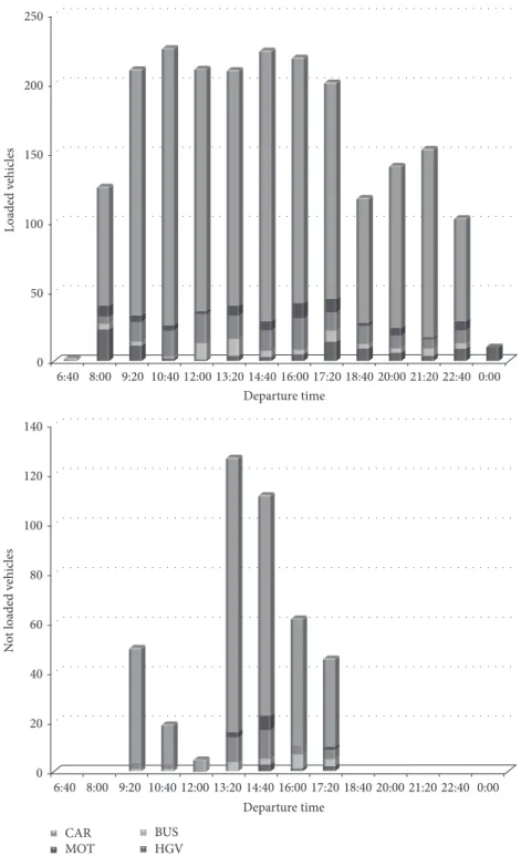
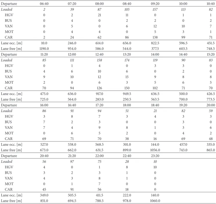
In the first simulation demand and supply were consid-ered as described above. In the second simulation demand was left unchanged while the frequency of the runs was halved, under the hypothesis of the unavailability of some ferries. The results, expressed in terms of vehicles embarking on any run of the ferry, are shown in Figures 9 and 10, respectively (numerical values are reported in Appendix).

Tables 4, 5, 6, and 7 show the values of the embarked vehicles in terms of filled space and vehicle numbers. The lane occupation parameter was used as indicator since the number of vehicles that can be embarked depends on the vehicular composition.

In the first simulation (Figure 9) the lane occupation parameter ranges from 10 to 949.5 meters (the number of vehicles embarked ranges from 2 to 174). In this scenario, all waiting vehicles are embarked on the ferry.

In the second simulation (Figure 10) the lane occupation parameter ranges from 10 to 1200 meters (the number of

(10)

0 50 100 150 200 250 6:40 8:00 9:20 10:40 12:00 13:20 14:40 16:00 17:20 18:40 20:00 21:20 22:40 0:00 L o aded v ehic les 0 20 40 60 80 100 120 140 6:40 8:00 9:20 10:40 12:00 13:20 14:40 16:00 17:20 18:40 20:00 21:20 22:40 0:00 N o t loaded v ehic les Departure time CAR MOT VAN BUS HGV Departure time

Figure 10: Vehicles embarking and remained on the pier for any run of the ferry, second simulation.

vehicles embarked ranges from 2 to 226). In this scenario, it happens that some vehicles cannot be embarked on the ferry. As an example, at time 9:20 the unloaded vehicles are 50, at 10:40 they are 19, and so on. Figure 11 shows the profile of the embarked vehicles, in terms of filled space. A peak (about 950 meters of filled space) can be seen at 13.20 hours for the first simulation and peak values from 9:20 to 17:20 for the second simulation.

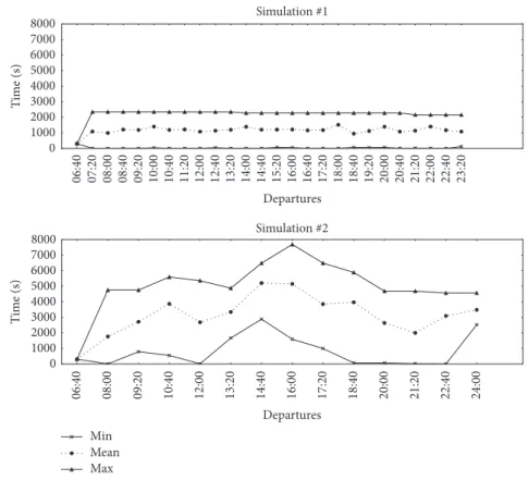
It has been possible to evaluate, for the two described sim-ulations, some statistics about the waiting times of vehicles and times for loading/unloading operations.

The waiting time for each vehicle on board of each run has been calculated as the difference between the departure time of the run of the ferry and the arrival time of the vehicle at the initial node of the boarding arc. Such values for the two simulations, expressed in seconds, are reported in

(11)

Table 4: Vehicles embarking on any run of the ferry, first simulation. Departure 06:40 07:20 08:00 08:40 09:20 10:00 10:40 Loaded 2 39 87 105 157 113 82 HGV 0 2 21 11 0 1 1 BUS 0 4 0 2 2 0 2 VAN 0 5 0 6 12 10 7 MOT 0 4 4 0 5 3 1 CAR 2 24 62 86 138 99 71 Lane occ. [m] 10.0 246.0 614.0 656.0 822.5 596.5 451.5 Lane free [m] 1190.0 954.0 586.0 544.0 377.5 603.5 748.5 Departure 11:20 12:00 12:40 13:20 14:00 14:40 15:20 Loaded 85 111 158 174 119 90 83 HGV 0 1 4 0 3 3 0 BUS 4 6 10 6 0 2 0 VAN 9 10 12 15 9 8 8 MOT 2 0 6 3 5 6 5 CAR 70 94 126 150 102 71 70 Lane occ. [m] 475.0 636.0 917.0 949.5 636.5 500.0 426.5 Lane free [m] 725.0 564.0 283.0 250.5 563.5 700.0 773.5 Departure 16:00 16:40 17:20 18:00 18:40 19:20 20:00 Loaded 86 91 94 51 21 82 59 HGV 3 8 7 3 4 3 3 BUS 7 2 3 0 0 3 0 VAN 7 4 9 8 1 3 6 MOT 0 6 5 2 0 4 2 CAR 69 71 70 38 16 69 48 Lane occ. [m] 527.0 538.0 568.5 301.0 144.0 457.0 335.0 Lane free [m] 673.0 662.0 631.5 899.0 1056.0 743.0 865.0 Departure 20:40 21:20 22:00 22:40 23:20 Loaded 56 97 75 28 10 HGV 4 0 1 8 10 BUS 3 2 3 1 0 VAN 4 3 8 1 0 MOT 0 1 7 0 0 CAR 45 91 56 18 0 Lane occ. [m] 349.0 505.5 411.5 222.0 140.0 Lane free [m] 851.0 694.5 788.5 978.0 1060.0

Appendix and profiles of the waiting time values (minimum, maximum, and mean value) for the two simulations are shown in Figure 12.

In the first simulation the waiting time (considering all the departure times) ranges from 4 to 2350 seconds; the mean of the wait time ranges from 310 to 1520 seconds. In the second one the waiting time (considering all the departure times) ranges from 5 to 7680 seconds; the mean of the waiting time ranges from 310 to 5199 seconds.

5. Conclusions

In this paper, the simulation of a multimodal transport system with a mesoscopic approach is discussed. En-route changes

of the transport modes are modelled to simulate users’ behaviour within a mesoscopic DNL framework. Model is extended to be applied in a multimodal context introducing two main aspects: the modal change of travellers and the aggregation of modal resources, describing how different modal resources can be aggregated in another one containing them. The operation of modal change is modelled by means of functional arcs (boarding and alighting arcs) introduced into the graph in correspondence of the node where the modal change is carried out.

A test application based on a real case has been developed considering the ferry services that guarantees the cross of the Strait of Messina (connecting Sicilia island with Calabria in the Italian peninsula). In particular, within the application,

(12)

Table 5: Vehicles embarking on any run of the ferry, second simulation. Departure 06:40 08:00 09:20 10:40 12:00 13:20 14:40 Loaded 2 126 211 226 211 210 224 HGV 0 23 11 2 1 4 3 BUS 0 4 3 1 12 12 4 VAN 0 5 14 19 21 17 15 MOT 0 8 5 4 2 7 7 CAR 2 86 178 200 175 170 195 Not loaded 0 0 50 19 5 127 112 HGV 0 0 0 0 3 BUS 1 1 0 4 2 VAN 3 2 0 10 12 MOT 0 0 0 2 6 CAR 46 16 5 111 89 Lane occ. [m] 10.0 860.0 1204.5 1202.0 1206.0 1203.5 1202.5 Lane free [m] 1190.0 340.0 0.0 0.0 0.0 0.0 0.0 Departure 16:00 17:20 18:40 20:00 21:20 22:40 24:00 Loaded 219 201 118 141 153 103 10 HGV 5 14 9 6 4 9 10 BUS 3 8 3 3 5 4 0 VAN 23 13 13 9 7 9 0 MOT 11 10 3 6 1 7 0 CAR 177 156 90 117 136 74 0 Not loaded 62 46 0 0 0 0 0 HGV 1 2 BUS 6 3 VAN 4 4 MOT 0 1 CAR 51 36 Lane occ. [m] 1202.5 1201.0 723.5 792.0 854.5 633.5 140.0 Lane free [m] 0.0 0.0 476.5 408.0 345.5 566.5 1060.0

users’ operations consisting in reaching the port terminal with wheeled vehicles (i.e., cars, vans, etc.) and changing transport mode (embarking the vehicle on a ferry) have been simulated.

Two scenarios have been considered: the first one repro-ducing the current state of the transport system; the second one assuming that frequency of ferries is halved. Some indicators obtained from the model (such as waiting time, loading, and unloading times) have been used to evaluate the performances of the transport system.

The evaluation of the loading/unloading operation times has been conducted by means of cost functions calibrated on real observations. Waiting times at terminals can be obtained for each vehicle and some statistics on these values have been used as performance indicators.

Another indicator consists in the respect of ferries’ capacity constrain that, in the reported example, consists of the number of vehicles that were not able to embark due to overcoming of the usable length of ferry cargo lane.

It is shown how the possibility to consider more trans-portation modes interacting each other can be effectively approached in a mesoscopic DNL framework.

Implementation of cost functions able to simulate transit systems operations and multimodal freight systems opera-tions is under development.

Appendix

Tables 4, 5, 6, and 7 report the numeric values obtained from simulation.

The entries of Tables 4 and 5 indicate the following: Departure: the departure time of the ferry as shown from the timetable; Loaded: the number of vehicles being embarked; Lane occ.: the length of ferry’s cargo lane occupied by the vehicles; Lane free: the length of ferry’s cargo lane being left; Not loaded: the number of vehicles that was not able to embark due to the capacity constraint of the ferry.

The entries of Tables 6 and 7 indicate the following: Departure: the departure time of the ferry as shown from the timetable; Wait min: the minimum value among waiting times of the vehicles on board the considered run; Wait max: the maximum value among waiting times of the vehicles on board the considered run; Wait mean: the mean waiting times of the vehicles on board the considered run; Wait sdev:

(13)

Simulation #1 Simulation #2 ca rg o la n e o ccu p ied F rac tio n o f f er ry’ s ca rg o la n e o ccu p ied F rac tio n o f f er ry’ s Departures Departures 06 :40 07 :20 08 :00 08 :40 09 :20 10 :00 10 :40 11 :20 12 :00 12 :40 13 :20 14 :00 14 :40 15 :20 16 :00 16 :40 17 :20 18 :00 18 :40 19 :20 20 :00 20 :40 21 :20 22 :00 22 :40 23 :20 06 :40 08 :00 09 :20 10 :40 12 :00 13 :20 14 :40 16 :00 17 :20 18 :40 20 :00 21 :20 22 :40 24 :00 1.0 0.8 0.6 0.4 0.2 0.0 1.0 0.8 0.6 0.4 0.2 0.0

Figure 11: Length of ferry’s cargo lane occupied by vehicles for each run.

8000 7000 6000 5000 4000 3000 2000 1000 0 Ti m e ( s) Simulation #2 Departures 06 :40 08 :00 09 :20 10 :40 12 :00 13 :20 14 :40 16 :00 17 :20 18 :40 20 :00 21 :20 22 :40 24 :00 Simulation #1 Departures 06 :40 07 :20 08 :00 08 :40 09 :20 10 :00 10 :40 11 :20 12 :00 12 :40 13 :20 14 :00 14 :40 15 :20 16 :00 16 :40 17 :20 18 :00 18 :40 19 :20 20 :00 20 :40 21 :20 22 :00 22 :40 23 :20 8000 7000 6000 5000 4000 3000 2000 1000 0 Ti m e ( s) Min Mean Max

(14)

Table 6: Waiting times for loading/unloading operations, first simulation. Departure 06:40 07:20 08:00 08:40 09:20 10:00 10:40 11:20 12:00 Wait min [s] 310 5 4 11 11 45 9 11 11 Wait max [s] 310 2350 2350 2350 2350 2349 2349 2347 2348 Wait mean [s] 310 1087 991 1212 1186 1403 1190 1220 1081 Wait sdev [s] 0 653 634 723 669 696 704 673 693 Loading [s] 12 325 788 807 983 706 542 580 775 Unloading [s] 10 292 719 721 856 609 475 509 687 Departure 12:40 13:20 14:00 14:40 15:20 16:00 16:40 17:20 18:00 Wait min [s] 50 7 9 12 71 57 8 16 13 Wait max [s] 2349 2348 2280 2280 2280 2280 2280 2280 2280 Wait mean [s] 1141 1198 1393 1204 1210 1218 1162 1179 1520 Wait sdev [s] 691 688 689 691 657 691 697 669 653 Loading [s] 1150 1146 764 619 511 660 678 713 365 Unloading [s] 1029 1006 665 543 439 594 607 631 313 Departure 18:40 19:20 20:00 20:40 21:20 22:00 22:40 23:20 Wait min [s] 70 58 70 13 23 16 5 125 Wait max [s] 2280 2280 2280 2280 2160 2160 2160 2160 Wait mean [s] 952 1122 1396 1083 1139 1405 1173 1083 Wait sdev [s] 750 657 686 728 698 649 640 649 Loading [s] 179 569 405 434 602 518 287 192 Unloading [s] 161 510 351 390 534 455 263 180

Table 7: Waiting times for loading/unloading operations, second simulation.

Departure 06:40 08:00 09:20 10:40 12:00 13:20 14:40 Wait min [s] 310 5 790 549 13 1667 2880 Wait max [s] 310 4750 4750 5589 5350 4868 6480 Wait mean [s] 310 1764 2712 3864 2681 3341 5199 Wait sdev [s] 0 1322 1188 1464 1581 898 955 Loading [s] 12 1113 1465 1422 1477 1497 1450 Unloading [s] 10 1011 1293 1232 1306 1334 1273 Departure 16:00 17:20 18:40 20:00 21:20 22:40 24:00 Wait min [s] 1591 994 69 70 23 5 2524 Wait max [s] 7680 6480 5880 4680 4680 4560 4560 Wait mean [s] 5144 3848 3966 2633 1996 3086 3482 Wait sdev [s] 1751 1573 1663 1247 1333 1343 649 Loading [s] 1463 1511 893 973 1036 806 192 Unloading [s] 1269 1352 786 861 924 718 180

the standard deviation of waiting times of the vehicles on board the considered run; Loading: time needed for loading operations for the vehicles on board the considered run; Unloading: time needed for unloading operations for the vehicles on board the considered run.

Competing Interests

The authors declare that there is no conflict of interests regarding the publication of this paper.

References

[1] A. Lozano and G. Storchi, “Shortest viable hyperpath in multi-modal networks,” Transportation Research Part B: Methodolog-ical, vol. 36, no. 10, pp. 853–874, 2002.

[2] R. van Nes, “Design of multimodal transport networks: a hierarchical approach,” TRAIL-Thesis Series T2002/5, TRAIL Research School, DUP Science, Delft, The Netherlands, 2002. [3] H. K. Lo, C. Yip, and K. Wan, “Modeling transfer and

non-linear fare structure in multi-modal network,” Transportation Research Part B: Methodological, vol. 37, no. 2, pp. 149–170, 2003.

(15)

[4] M. E. T. Horn, “An extended model and procedural framework for planning multi-modal passenger journeys,” Transportation Research Part B: Methodological, vol. 37, no. 7, pp. 641–660, 2003. [5] H. Ayed, C. Galvez-Fernandez, Z. Habbas, and D. Khadraoui, “Solving time-dependent multimodal transport problems using a transfer graph model,” Computers and Industrial Engineering, vol. 61, no. 2, pp. 391–401, 2011.

[6] D. Kirchler, L. Liberti, and R. Wolfler Calvo, “A label correcting algorithm for the shortest path problem on a multi-modal route network,” in Proceedings of the 11th International Conference on Experimental Algorithms, Bordeaux, France, June 2012, vol. 7276 of Lecture Notes in Computer Science, pp. 236–247, Springer, 2012.

[7] D. Ambrosino and A. Sciomachen, “An algorithmic framework for computing shortest routes in urban multimodal networks with different criteria,” Procedia—Social and Behavioral Sci-ences, vol. 108, pp. 139–152, 2014.

[8] L. dell’Olio, A. Ibeas, P. Cec´ın, and F. dell’Olio, “Willingness to pay for improving service quality in a multimodal area,” Trans-portation Research Part C: Emerging Technologies, vol. 19, no. 6, pp. 1060–1070, 2011.

[9] T. A. Arentze and E. J. E. Molin, “Travelers’ preferences in mul-timodal networks: design and results of a comprehensive series of choice experiments,” Transportation Research Part A: Policy and Practice, vol. 58, pp. 15–28, 2013.

[10] D. Wu, Y. Yin, S. Lawphongpanich, and H. Yang, “Design of more equitable congestion pricing and tradable credit schemes for multimodal transportation networks,” Transportation Re-search Part B: Methodological, vol. 46, no. 9, pp. 1273–1287, 2012. [11] R.-R. Shi and Z.-C. Li, “Pricing of multimodal transportation networks under different market regimes,” Journal of Trans-portation Systems Engineering and Information Technology, vol. 10, no. 5, pp. 91–97, 2010.

[12] C. F. Daganzo, “System optimum and pricing for the day-long commute with distributed demand, autos and transit,” Transportation Research Part B: Methodological, vol. 55, pp. 98– 117, 2013.

[13] E. Cascetta, F. Russo, F. A. Viola, and A. Vitetta, “A model of route perception in urban road networks,” Transportation Research Part B: Methodological, vol. 36, no. 7, pp. 577–592, 2002. [14] A. Quattrone and A. Vitetta, “Random and fuzzy utility models for road route choice,” Transportation Research Part E: Logistics and Transportation Review, vol. 47, no. 6, pp. 1126–1139, 2011. [15] P. Modesti and A. Sciomachen, “A utility measure for finding

multiobjective shortest paths in urban multimodal transporta-tion networks,” European Journal of Operatransporta-tional Research, vol. 111, no. 3, pp. 495–508, 1998.

[16] A. Spickermann, V. Grienitz, and H. A. von der Gracht, “Head-ing towards a multimodal city of the future?: multi-stakeholder scenarios for urban mobility,” Technological Forecasting and Social Change, vol. 89, pp. 201–221, 2014.

[17] A. Kramers, “Designing next generation multimodal traveler information systems to support sustainability-oriented deci-sions,” Environmental Modelling & Software, vol. 56, pp. 83–93, 2014.

[18] M. Diana, “From mode choice to modal diversion: a new behavioural paradigm and an application to the study of the demand for innovative transport services,” Technological Fore-casting and Social Change, vol. 77, no. 3, pp. 429–441, 2010.

[19] M. Diana, “Measuring the satisfaction of multimodal travelers for local transit services in different urban contexts,” Trans-portation Research Part A: Policy and Practice, vol. 46, no. 1, pp. 1–11, 2012.

[20] G. E. Cantarella, “A general fixed-point approach to multimode multi-user equilibrium assignment with elastic demand,” Trans-portation Science, vol. 31, no. 2, pp. 107–128, 1997.

[21] E. Fernandez, J. de Cea, M. Florian, and E. Cabrera, “Network equilibrium models with combined modes,” Transportation Science, vol. 28, no. 3, pp. 182–192, 1994.

[22] R. Garc´ıa and A. Mar´ın, “Network equilibrium with combined modes: models and solution algorithms,” Transportation Re-search Part B: Methodological, vol. 39, no. 3, pp. 223–254, 2005. [23] Z. Liu and Q. Meng, “Bus-based park-and-ride system: a sto-chastic model on multimodal network with congestion pricing schemes,” International Journal of Systems Science, vol. 45, no. 5, pp. 994–1006, 2014.

[24] S. Bajwa, G. Tamamoto, M. Kuwahara, E. Chung, and S. Tanaka, “A dynamic multi-modal transport simulation model,” 2005, http://www.jsce.or.jp/library/open/proc/maglist2/00039/ 200511 no32/pdf/7.pdf.

[25] E. Cascetta and G. E. Cantarella, “A day-to-day and within-day dynamic stochastic assignment model,” Transportation Research Part A: General, vol. 25, no. 5, pp. 277–291, 1991.

[26] H. B. Celikoglu, “A dynamic network loading process with explicit delay modelling,” Transportation Research Part C: Emerging Technologies, vol. 15, no. 5, pp. 279–299, 2007. [27] M. Carey and M. McCartney, “Behaviour of a whole-link travel

time model used in dynamic traffic assignment,” Transportation Research Part B: Methodological, vol. 36, no. 1, pp. 83–95, 2002. [28] B.-W. Wie, R. L. Tobin, D. Bernstein, and T. L. Friesz, “A compar-ison of system optimum and user equilibrium dynamic traffic assignments with schedule delays,” Transportation Research Part C, vol. 3, no. 6, pp. 389–411, 1995.

[29] J. H. Wu, Y. Chen, and M. Florian, “The continuous dynamic network loading problem: a mathematical formulation and solution method,” Transportation Research Part B: Methodolog-ical, vol. 32, no. 3, pp. 173–187, 1998.

[30] H. B. Celikoglu, “A dynamic network loading model for traffic dynamics modeling,” IEEE Transactions on Intelligent Trans-portation Systems, vol. 8, no. 4, pp. 575–583, 2007.

[31] S. Han, “Dynamic traffic modelling and dynamic stochastic user equilibrium assignment for general road networks,” Transporta-tion Research Part B: Methodological, vol. 37, no. 3, pp. 225–249, 2003.

[32] M. Dell’Orco, “A dynamic network loading model for mesosim-ulation in transportation systems,” European Journal of Opera-tional Research, vol. 175, no. 3, pp. 1447–1454, 2006.

[33] K. Er-Rafia, M. Florian, M. Mahut, and S. Velan, “Three ap-proaches to the dynamic network loading problem,” in Proceed-ings of the IEEE Intelligent Transportation Systems Conference, pp. 127–131, Oakland, Calif, USA, August 2001.

[34] E. Castillo, J. M. Menéndez, M. Nogal, P. Jiménez, and S. Sánchez-Cambronero, “A FIFO rule consistent model for the continuous dynamic network loading problem,” IEEE Transac-tions on Intelligent Transportation Systems, vol. 13, no. 1, pp. 264– 283, 2012.

[35] C. F. Daganzo, “The cell transmission model, part II: network traffic,” Transportation Research Part B: Methodological, vol. 29, no. 2, pp. 79–93, 1995.

(16)

[36] M. J. Smith, “The existence of a time-dependent equilibrium distribution of arrivals at a single bottleneck,” Transportation Science, vol. 18, no. 4, pp. 385–394, 1984.

[37] H. S. Mahmassani, M. Saberi, and K. Ali Zockaie, “Urban net-work gridlock: theory, characteristics, and dynamics,” Proce-dia—Social and Behavioral Sciences, vol. 80, pp. 79–98, 2013. [38] M. Gao, “A node model capturing turning lane capacity and

physical queuing for the dynamic network loading problem,” Mathematical Problems in Engineering, vol. 2012, Article ID 542459, 14 pages, 2012.

[39] Y. W. Xu, J. H. Wu, M. Florian, P. Marcotte, and D. L. Zhu, “Advances in the continuous dynamic network loading prob-lem,” Transportation Science, vol. 33, no. 4, pp. 341–353, 1999. [40] H. B. Celikoglu and M. Dell’Orco, “Mesoscopic simulation of a

dynamic link loading process,” Transportation Research Part C: Emerging Technologies, vol. 15, no. 5, pp. 329–344, 2007. [41] H. B. Celikoglu, E. Gedizlioglu, and M. Dell’Orco, “A

node-based modeling approach for the continuous dynamic network loading problem,” IEEE Transactions on Intelligent Transporta-tion Systems, vol. 10, no. 1, pp. 165–174, 2009.

[42] N. C. Balijepalli, D. Ngoduy, and D. P. Watling, “The two-regime transmission model for network loading in dynamic traffic assignment problems,” Transportmetrica A: Transport Science, vol. 10, no. 7, pp. 563–584, 2014.

[43] M. T. S´anchez-Rico, R. Garc´ıa-R´odenas, and J. L. Espinosa-Aranda, “A monte carlo approach to simulate the stochastic demand in a continuous dynamic traffic network loading prob-lem,” IEEE Transactions on Intelligent Transportation Systems, vol. 15, no. 3, pp. 1362–1373, 2014.

[44] M. P. Linares, J. Barcel´o, C. Carmona, and C. Monta˜nola-Sales, “Validation of a new multiclass mesoscopic simulator based on individual vehicles for dynamic network loading,” in Proceed-ings of the Winter Simulation Conference, pp. 2048–2059, 2014. [45] M. Di Gangi, “Modeling evacuation of a transport system:

appli-cation of a multimodal mesoscopic dynamic traffic assignment model,” IEEE Transactions on Intelligent Transportation Systems, vol. 12, no. 4, pp. 1157–1166, 2011.

[46] G. Delfino, D. Iann`o, C. Rindone, and A. Vitetta, Stretto di Messina: uno Studio della Mobilit`a Intermodale per i Passeggeri, Alfagi, Villa S. Giovanni, Italy, 2011.

[47] F. Russo and A. G. Cartisano, “Analytical models for Ro-Ro and Lo-Lo terminals in a multipurpose port,” WIT Transactions on the Built Environment, vol. 62, pp. 79–87, 2002.

(17)

International Journal of