Ph.D. in Methods, models and technologies for
engineering
XXXII Cycle
Ph.D. thesis
Application of Machine Learning Techniques to
Brain Magnetic Resonance Imaging in
Hypertensive Patients
Supervisor
Ph.D. student
Prof. Francesco Tortorella
Lorenzo Carnevale
Coordinator
Prof.ssa Wilma POLINI
thesis work, improving it with his insightful observation.
I want to thank my mentor Prof. Giuseppe Lembo, which gave me the cultural, technical and human foundation to achieve this result and many others achieved during my collaboration with his research group. Without his support throughout the years I would not be the person I am.
Thanks to my sister Prof. Daniela Carnevale, which is the example I follow since my first steps. I could not ask for a better trail to observe and take as a model. Thanks to all my co-workers and colleagues, supporting this work and many others performed during these years.
Finally, thanks to all my family which supported me in every step of my studies. This support has been the foundation of all my journey, and no word will be good enough to recapitulate my gratitude.
I
the early effects of vascular risk factors on the brain. In this thesis we will tackle the problem of hypertensive brain organ damage characterization approaching it at multiple scales and leveraging multiple techniques. The first part of the thesis will be focused on a deep learning system to perform automatic segmentation of White Matter Hyperintensities (WMH), one of the most common form of macrostructural vascular injury in the brain, on T2-FLAIR imaging. To this aim we will leverage a public dataset and compare our results with the ones achieved in the MICCAI WMH segmentation challenge. The second part of the thesis is focused on the setup of analysis pipelines for Diffusion Tensor Imaging (DTI) and resting state functional MRI (rs-fMRI), with the aim of characterize the microstructural integrity and the functional connectivity. These pipelines have been implemented on hypertensive brains to characterize the subtle brain functional and microstructural damage associated with the hypertensive condition. Finally, both approaches have been implemented in a ongoing research program at IRCCS Neuromed in the context of the heart and brain clinical research, achieving the injury characterization for the first two recruited patients of the study and field-testing the proposed brain injury characterization framework.
II
TABLE OF CONTENTS
Abstract ... II List of Figures ... V
List of Tables ... 1
CHAPTER 1. Introduction and background ... 2
1.1 Introduction ... 2
1.2 Hypertension ... 3
1.3 The brain and the cerebrovascular system ... 4
1.3.1 Anatomy of the Brain ... 4
1.3.2 The cerebrovascular tree and the neurovascular unit ... 5
1.4 Magnetic Resonance Imaging ... 6
1.5 The Role of Machine Learning ... 7
1.6 Outline of the work and aims ... 8
CHAPTER 2. A deep learning approach for the segmentation of White Matter Hyperintensities 10 2.1 Introduction ... 10
2.2 MRI applied to evaluate macrostructural brain damage: White Matter Hyperintensities ... 12 2.3 Methods ... 15 2.3.1 Dataset Characteristics ... 15 2.3.2 Brain Extraction ... 16 2.3.3 Framework ... 16 2.3.4 Preliminary Experiments ... 17 2.3.5 Network Architectures ... 18 2.3.6 Training ... 20 2.3.7 Evaluation Metrics ... 21
III
2.4 Results ... 22
2.4.1 Raw Data ... 22
2.4.2 Normalized Data ... 25
2.5 Discussion ... 27
CHAPTER 3. Hypertensive patients and early brain damage: a structural and functional connectivity characterization ... 30
3.1 Introduction ... 30
3.1.1 Patient Sample ... 31
3.2 Structural Connectivity: Diffusion Tensor Imaging applied to Hypertensive Patients ... 33
3.2.1 Diffusion parameters ... 34
3.2.2 From tensorial model to probabilistic diffusion modelling... 37
3.2.3 Probabilistic tractography ... 38
3.2.4 Analysis Pipeline ... 39
3.3 Functional Connectivity: resting state functional MRI applied to Hypertensive Patients ... 42
3.3.1 Functional Network Analysis ... 43
3.3.2 Graph Analysis ... 46
3.3.3 Analysis Pipeline ... 47
3.4 Results ... 49
3.4.1 Hypertension alters microstructural integrity of white matter ... 49
3.4.2 WM microstructural alterations scale with cognitive impairment and target organ damage ... 53
3.4.3 ROI-to-ROI analyses of Functional Connectivity show altered aberrant connections between task-positive networks ... 55
3.4.4 Graph Theory Analyses of brain network connectivity ... 56
3.4.5 Diffusion parameters and cognitive performances correlates with the functional connectivity ... 57
3.5 Dataset Construction ... 58
CHAPTER 4. A machine learning approach to classify hypertension from advanced neuroimaging data ... 59
IV
4.1 The curse of dimensionality ... 59
4.2 Weka Tools ... 60 4.3 Classifiers ... 60 4.3.1 J48 Decision Tree ... 60 4.3.2 Naïve Bayes ... 61 4.3.3 Logistic Regression ... 61 4.3.4 SVM ... 62 4.4 Ensemble ... 63 4.4.1 AdaBoost ... 63 4.4.2 Bagging ... 63 4.4.3 Random Forest ... 64 4.4.4 Random Subspace ... 64 4.5 Feature Selection ... 64
4.5.1 Correlation-based Feature Subset ... 65
4.5.2 Information Gain and Gain Ratio ... 65
4.5.3 Principal Component Analysis ... 65
4.6 Results ... 66
4.6.1 Global Comparison ... 66
4.6.2 Global Ranking ... 68
4.6.3 Discussion ... 70
CONCLUSIONS ... 72
Application of our pipeline analysis to two clinical cases ... 72
RF004 ... 72
RF009 ... 74
Conclusion ... 76
Appendix A – MRI Sequences ... 77
Appendix B – Network Structures ... 86
V
L
IST OF
F
IGURES
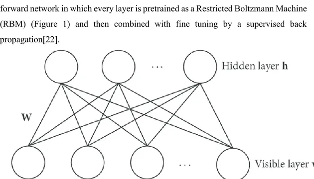
Figure 1- Restricted Boltzmann Machine Model ... 10
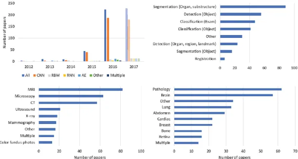
Figure 2- Occurrences of deep learning research papers in medical imaging ... 11
Figure 3 – Example of T2 Flair images with segmented WMH (in green) and lesions of other nature (Red). Top row: scan of a patient with a low grade WMH (Fazekas 1); Middle row: scan of a patient with severe WMH (Fazekas 4); Bottom Row: same image without segmentation overlays ... 14
Figure 4 – Left: T2 Flair showing similar intensity between WMH and skin. Right: mask of the extracted brain in red, with WMH segmentation in green. ... 16
Figure 5 - Schematics of MIScnn framework implementation ... 17
Figure 6 - 3D Train and Validation loss ... 18
Figure 7 - Comparison between 3D patch and 2D patch ... 19
Figure 8 – U-NET standard architecture ... 19
Figure 9 - Variation of final evaluation metrics with epochs ... 23
Figure 10 - Loss trend with raw data. Left column: Unet, Right column: Fractal Net ... 24
Figure 11 - Loss trend with normalized data. Left column: Unet, Right column: Fractal Net ... 26
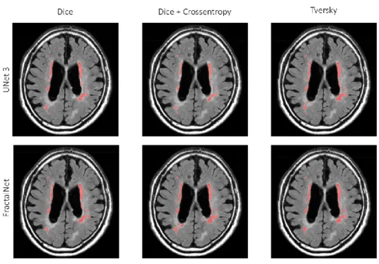
Figure 12 - Segmentation results of all the implemented models on normalized data ... 27
Figure 13 - Triplane comparison between ground truth (top row) and segmentation results of our proposed system (bottom row) ... 28
Figure 14 - Enrollment Flowchart ... 31
Figure 15 - Diffusion Parameters Map... 35
Figure 16 - Fractional Anisotropy Color Map ... 36
Figure 17 - Probabilistic Diffusion Modelling ... 38
Figure 18 - Probabilistic Tractography Heathmap ... 39
Figure 19 – DTI Analysis Pipeline ... 40
Figure 20 - White matter tracts reconstruction ... 42
VI
Figure 22 - Yeo et al. coarse (7-network) cortex parcellation ... 44
Figure 23 - Connectome Ring Display ... 45
Figure 24 - Graph network built on rs-fMRI ... 47
Figure 25 - rs-fMRI Analysis Pipeline ... 48
Figure 26 - WM altered tracts ... 50
Figure 27 - Characteristic pattern of altered tracts and DTI-organ damage correlations ... 54
Figure 28 - Connectome ring showing altered subnetwork and its 3D reconstruction ... 56
Figure 29 - Nodes altered in corresponding graph metrics ... 57
Figure 30 - Linearly separable data ... 62
Figure 31 - Optimal hyperplane placement ... 63
Figure 32 - Input image, raw WMH segmentation and masked WMH segmentation of patient RF004 ... 73
Figure 33 - Input image, raw WMH segmentation and masked WMH segmentation of patient RF009 ... 75
Figure 34 ... 78
Figure 35 ... 79
Figure 36 ... 80
Figure 37 – Pulse sequence of FLAIR sequence ... 80
Figure 38 - Diffusion Tensor... 83
1
L
IST OF
T
ABLES
Table 1 - Results for Raw Data ... 25
Table 2 - Results for Normalized Data ... 25
Table 3 - Patient Sample Characteristics ... 32
Table 4 - Cognitive Assessment ... 33
Table 5 - MoCA cognitive subdomains ... 33
Table 6 - Average FA and MD of segmented tracts ... 51
Table 7 - Average AD and RD of segmented tracts... 52
Table 8 - Top 5 classifiers on functional data ... 66
Table 9 - Top 5 classsifiers on advanced neuroimaging data ... 67
Table 10 - Top 5 classifiers on all data ... 67
Table 11 - Accuracy Ranking ... 68
Table 12 - F Measure Ranking ... 69
2
CHAPTER 1.
I
NTRODUCTION AND
BACKGROUND
1.1 Introduction
With the worldwide increase of ageing population, dementia and neurodegenerative diseases became a major issue for healthcare systems that have to ensure adequate management of affected subjects. The estimates by World Health Organization report of more than 35 million people worldwide affected by dementia and is expected a 3-fold increase by year 2050[1]. One of the main modifiable risk factors leading to these pathologies is hypertension[2], a chronic condition affecting about the 30% of adult population worldwide, with incidence growing to more than 60% in the elderly. It is a consolidated knowledge in both clinical practice and pre-clinical research that high blood pressure exerts powerful detrimental effect on a variety of organs such as heart and kidneys, while its effect on cognition and brain health are less known and needs further investigation.
Recent works have leveraged post-mortem analysis tools to shed light on the pathophysiological conditions underlying the symptoms of dementia or cognitive impairment. These works evidenced that more than 50% of dementia cases shown a vascular involvement, as main factor or in combination with neurodegeneration[3]. To empower clinicians and give them proficient tools to understand whether the cognitive decline in process is codetermined by vascular factors, first of all we should investigate the effects on brain structure and functioning of primary vascular risk factors and pathological conditions, as hypertension[4, 5].
To this aim, it is fundamental to correctly stage the entity of the injuries produced by the hypertensive pathology on different brain regions and how the progression of the pathology impacts its structure and functional organization. Magnetic Resonance
3
Imaging (MRI) has proven itself as an unparalleled tool to investigate these characteristics in vivo in a non-invasive manner and without administering ionizing radiations to the patient. Leveraging different kind of MRI scans, we can obtain various information about the brains, investigating with the appropriate tools different markers corresponding to distinct stages of the pathology.
1.2 Hypertension
Hypertension has been classically defined as systolic blood pressure (SBP) > 140 mmHg and/or diastolic blood pressure (DBP) >90 mmHg, or the use of antihypertensive medication. Hypertension is a complex and systematic pathology, affecting primary the cardiovascular system, with a multitude of secondary organs and functions involved by the effects of long-lasting elevated blood pressure. The hypertension diagnosis and treatment is carried on according to guidelines established and published by two major international workgroups: i) the join American Heart Association and American College of Cardiology Hypertension guidelines (AHA/ACC)[6]; ii) the European Society of Cardiology Hypertension guidelines (ESC)[7]. It is worth noting that while the two workgroups have been substantially concordant on the aforementioned hypertension definition throughout the history, the last revision of the AHA/ACC guidelines has defined as hypertensive also the subject reporting a SBP > 130mmHg and/or a DBP >80 mmHg. This change reflected in a more intensive use of anti-hypertensive treatment, looking for an increased benefit on both well-known and object of research consequences of hypertension[8].
While the end-organ damage induced by hypertension in some districts like heart or kidneys is comprehensively characterized and studied, the effects of hypertension on the brain are largely unknown, with the main contribution identified as a strong risk factor for stroke and Alzheimer’s Disease. It is however becoming clearer thanks to recent mechanistic and epidemiologic studies that hypertension alone can impact cognition and can alter the cerebral homeostasis in a way capable of altering the cognitive performances of hypertensive patients, without the onset of neurological conditions as AD or acute cerebrovascular event[3, 9, 10].
4
1.3 The brain and the cerebrovascular system
The brain is the main organ of the nervous system, responsible for the perception and cognition. It is a complex organ made of billions of interconnected cells, which can be grouped respect to their anatomical or functional nature. One of the biggest efforts of contemporary neuroscience has been directed to map the differences between the different regions of the brain and to elucidate their distinct role in the cognition processes.
1.3.1 Anatomy of the Brain
The brain is made up of different major parts connected between them and attached to the spinal cord through the brainstem. This serves as a regulator of primary functions through the vagus nerve such as breathing, cardiac rhythm, digestive system, immune system activation. Attached to the brainstem there is the cerebellum, a neuronal structure mainly responsible for receiving sensory input from the peripheral nerves and managing the motor response. At the top of the brainstem we can find the limbic system, made of several substructures which are fundamental in several function as memory, learning and emotional responses.
The most important structure of the brain is the cerebrum, divided into left and right hemisphere interconnected by a central structure of thick neuronal fibers called corpus callosum. In the cerebrum we can distinguish the gray matter (GM) and white matter (WM), with the cerebrospinal fluid (CSF) filling the void spaces called ventriculi between different hemispheres and regions. The gray matter, named also the cortex, is the region composing the surface of the brain, is structured as a layered architecture of neuronal cell bodies interconnected between them on a single layer and between layers. The white matter instead is mainly composed by the neuronal axons connecting different brain regions. The most prominent characteristic of human brain respect to other species is the presence of convolutions, with crests named gyri and the valleys named sulci. This convoluted structure results in a greater surface of gray matter respect to the surface who would be available on a smooth sphere.
5
The main activity of the brain has been classically identified as cortical activity and with several techniques throughout the history we have been able to map with notable precision the regions of the cortex pairing them with their functions.
White matter, responsible for the intercommunications between distinct subcortical and cortical regions, can be divided in fascicles or bundles, which are organized groups of axons projecting in the same direction. Both grey and white matter mapping and organization will be discussed in further detail in Chapter 3.
1.3.2 The cerebrovascular tree and the neurovascular unit
While the brain is one of the most complex and energy demanding organs of our body, it is not provided with a proper energy storage, relying its functioning only on nutrients continuously coming through the cerebral circulation. Thus, to have a reliable cognitive functioning it is mandatory to get a constant and well-regulated blood flow feeding neuronal cells. To do so, the cerebrovascular tree has developed the capability to regulate its pressure and flow autonomously respect to the general circulation, namely the cerebral autoregulation. Alterations of this property following acute cerebrovascular events, due to sustained increase of blood pressure or the aging process can impact on cognitive performance, making the system less prone to distribute the nutrients from the blood flow equally in all the cerebral regions.To provide a homogeneous perfusion of the brain tissues, the large arteries branch into progressively smaller vessels, up to the diameter of few microns composing the capillary bed. The complex of cells responsible for the mechanism of isolating the neuronal tissues from the direct blood flow running through the capillary bed is called the NeuroVascular Unit (NVU), mainly maintaining the integrity of the blood-brain barrier (BBB) and regulating the regional cerebral blood flow and oxygen and nutrient delivery[11].
Both large vessels and the NVU are part of the delicate mechanism of brain blood flow regulation, which is heavily stressed in conditions of hypertension and are two of the main target of damage in case of chronic elevated blood pressure, often reflected into an increased permeability of the BBB and other kinds of focal tissue damage, like white matter hyperintensities (discussed in detail in Chapter 2).
6
1.4 Magnetic Resonance Imaging
To date, the best available tool to explore the human brain is Magnetic Resonance Imaging (MRI). Originated around fifty years ago, this technology leverages the property of hydrogen nuclei which, when stimulated by radiofrequency pulses, resonate with the magnetic field where they are immersed, allowing the analysis of different tissues. By reading the signals emitted during the resonance we can obtain the time needed for a particular tissue to return to steady state on the longitudinal component or on the transverse one, respectively T1 relaxation time and T2 relaxation time. The images are obtained by weighting one of the two components, emphasizing the contrasts between tissues with different T1 or T2 relaxation times. During the decades, MRI techniques evolved from the methods that allowed to obtain images of internal tissues of the patients to techniques capable of providing functional insights of the biological systems under examination.
The support of various MRI techniques can be a fundamental addition to the clinical practice, in order to specifically characterize and diagnose different forms of cognitive impairment originated from vascular pathologies. On this notice, a modern and quantitative approach can be instrumental to extrapolate effective biomarkers for clinical and modern computer-driven analyses.
The first applications of brain MRI were developed to understand and analyse the morphological alterations induced by various pathologies impacting on white and grey matter. The first approach was aimed at obtaining a segmentation of the brain and a parcellation of the cortical areas, by hand or by using specialized software [12, 13]. The data obtained from these elaborations were used to characterize the neurodegenerative processes and put in relation the affected physical areas with the associated cognitive functions[14].
The development of new techniques specific for white matter injury evaluation paved the way to the analysis and identification of one of the most important markers of cerebrovascular damage in the brain: the white matter hyperintensities (WMH). T2-FLAIR sequence (T2-Fluid Attenuated Inversion Recovery, discussed in detail in Appendix A)[15] is useful to highlight regions of T2 prolongation in the white matter,
7
corresponding to regions of increased water content respect to normal white matter. In this kind of sequence, areas of hyperintensity represent a region where the white matter is undergoing a process of demyelination or axonal loss. In general, these alterations are the main evidence of cerebrovascular diseases, even though they can correspond to different pathological states[16].
Characterization of WMH has been first qualitative, with a grading system based on the appearance and position of the identifiable lesions[17], then with the progress of computer-aided diagnosis (CADx) systems and improvements in the computer vision field, we can now absolutely quantify the volume of white matter lesions[18, 19]. This improvement is fundamental to define absolute and quantitative biomarkers that could help in better evaluating and predicting the onset of VCI in the population at risk.
Further techniques of MRI were implemented to describe microstructural and functional alterations in the brain, respectively the diffusion tensor imaging and the functional magnetic resonance imaging. These techniques will be leveraged to describe the hypertensive brains and will be discussed in detail in next chapters of this thesis together with the analysis pipelines necessaries to get significant insight from the raw diffusion and functional data.
1.5 The Role of Machine Learning
Machine Learning is a branch of computer science aimed at designing automated systems capable of automatic learning from examples with minimal human guidance and interference. This results in computer programs capable of absorbing data, build and refine models on the input data to maximize the system capability to predict certain outcomes and perform better decision on new data.
The model adopted for the process of learning divides the ML algorithms in two major categories: supervised and unsupervised methods.
Supervised learning is based on a labelled training data set, in which every sample is associated to a distinct category. The main aim of the algorithm is to achieve the capability to generalize the decision took from the model (the classification) from the training data to unseen data.
8
Unsupervised learning is based on a heterogeneous data set without any labelling. The aim of the algorithm is to identify commonalities between different samples in the dataset and organize them in homogeneous group, the clusters.
The technological advances which took place in the last decade greatly improved the capabilities of training complex mathematical models with big datasets. Previous limitations were upper bounds in term of high-speed memory, needed to load the model, and the lack of adequate computing capabilities, needed to train complex models with a sufficient amount of data. Graphical Processing Unit (GPU) improvements were key to develop affordable and reliable parallel computing capability, exploiting the intrinsic parallel architecture needed for graphical computations: many processors needed for simple parallel operations to generate and perform calculations on matrix objects (i.e. images).
Neural Networks are one of the first models of machine learning proposed in literature, and while effective have been soon put aside due to the computational complexity of the training process. The model is made up by several primitive elements (the neurons) interconnected between them and whose connections are ruled by a rule which considers both their value and the value of incoming connections. This kind of model gives the flexibility of a common operator which can approximate any nonlinear function, given a particular architecture of connections is provided.
The intrinsic parallel nature of Neural Networks gave it a strong boost with recent technological leap, facilitating the training of architectures composed by several interconnected layer, composing “deep” networks.
1.6 Outline of the work and aims
In this thesis we will split the task of characterizing the brain injury associated with hypertension in two sections, both part of the heart and brain research program carried on at Istituto di Ricovero e Cura a Carattere Scientifico Neuromed by the AngioCardioNeurology and Translational Medicine department. The first one will tackle the segmentation of white matter hyperintensities, macroscopical lesions which are evidenced by MRI scans performed in the clinical routine, hallmark of advanced stage hypertension brain damage[20, 21]. To do so, we will leverage a publicly
9
available dataset comprising scans from different machines and clinical units in Europe. The second part will be centred on characterizing by advanced neuroimaging sequences the damage exerted on brain microstructure and functional organization by hypertension, in an early stage of pathology to design a multimodal biomarker which could be a candidate for prediction of cognitive decline[9]. This study will be conducted on patients recruited in our clinical unit, to set up all the neuroimaging pipelines to obtain a comprehensive microstructural and functional characterization of the brain. At this stage, it will be used to evaluate whether it is possible to predict the presence of a cardiovascular pathology only from neuroimaging analysis.
In both sections we will apply machine learning strategies, to leverage the amount of data generated from these experimental procedures and to automate the time-consuming part of labelling and quantification of lesion, with the final aim to produce a framework to comprehensively characterize the damage in the brains of hypertensive patients, from the earliest stage of it to identify the set of markers which can identify patients at risk of cognitive decline in the later stage of the pathology to automated tools to provide fast and reliable segmentation of hypertensive lesions in the brain to stratify in an efficient way the hypertensive population for their brain damage.
Our final aim will be to implement both strategies on patients recruited in our clinical unit in the context of an ongoing prospective study, to characterize patients in a longitudinal way to predict the onset of hypertension associated cognitive impairment from macrostructural, microstructural and functional data. Due to the ongoing recruiting process, it will be only shown the application of the complete pipeline to two example cases.
10
CHAPTER 2. A
DEEP LEARNING
APPROACH FOR THE SEGMENTATION OF
W
HITE
M
ATTER
H
YPERINTENSITIES
2.1 Introduction
The term “Deep Learning” and the concept of deep neural networks (DNN) was introduced in 2006 by Hinton in a seminal paper in which he showed a multilayer forward network in which every layer is pretrained as a Restricted Boltzmann Machine (RBM) (Figure 1) and then combined with fine tuning by a supervised back propagation[22].
After this first experiments an increasing number of problems were tackled by deep learning, especially in the context of computer vision and image processing with the Convolutional Neural Network (CNN) architecture. The capability of CNNs of
11
efficiently solving problems with results unmatched by other ML techniques soon captured the global attention of the computer vision and pattern recognition world, generating dozens of different architectures to solve different problems of different context.
The first successful applications of DNN has certainly been the image processing and recognition context: the ImageNET competition[23], a benchmark problem for image recognition, has seen a spike of the classification performance with the DNNs, from a 25% error percentage in 2010 with classical ML algorithm to a 4% classification error in 2015[24], implementing a complex CNN and achieving a performance superior to the human. Other fields of application which saw dramatic improvements with DNN are notably the Natural Language Processing (NLP), in which different kind of architectures have greatly improved the capability of machine to understand and process human written or spoken language, with great breakthroughs achieved in text sentiment analysis or speech recognition.
Medical imaging also saw great improvements from the implementation of deep learning approaches. Computer-aided diagnosis or and computer-aided detection (CADx) have always been one of the main research field in biomedical and computer engineering[25], with deep learning these systems have reached notable performances
12
in selected fields of application, like a CADx system for melanoma diagnosis which outperformed trained physicians in recognizing and grading melanomas from moles pictures[26].
Mimicking the capillary diffusion that deep learning had in several computer science, the medical imaging field has seen a sudden surge in the number of systems and research papers which implement deep learning strategies. As seen in Figure 2, from Litjens et al.[27], the breakthrough seen in 2012-2013 brought a 20x times appearance of deep learning techniques first in workshops and conferences, then in peer-reviewed journals. The breakdown of the task addressed in the papers and the imaging modalities in exam show that segmentation task is the most prominent one, often paired with MRI modality (see [27, 28] for comprehensive review). The most common model of NN is the Convolutional Neural Network, given its strong performance with image recognition and pattern recognition.
In my research experience I focused on neuroimaging analysis, with images obtained by various techniques of Magnetic Resonance Imaging (MRI). The first problem tackled with deep learning was the automatic segmentation of white matter lesions evidenced by T2-FLAIR imaging.
2.2 MRI applied to evaluate macrostructural brain
damage: White Matter Hyperintensities
MRI is a powerful tool for diagnosis of many different pathologies and the in-vivo inspection of internal organs. Thanks to the high contrast achieved between different soft tissues has established as the exam of choice for brain imaging, leveraging the different magnetic properties of gray matter, white matter and cerebrospinal fluid. During the last 50 years of clinical use of the MRI capabilities expanded greatly, and one of the first advanced sequences adopted in the routine examination has been the T2 Fluid Attenuated Inversion Recovery (FLAIR) (see Appendix A – MRI sequences for more information).
This kind of technique has been developed to image the brain weighting in T2 while attenuating the signal generated from the cerebrospinal fluid. In this way, while gray
13
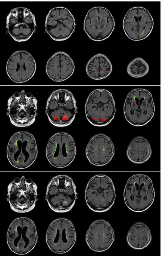
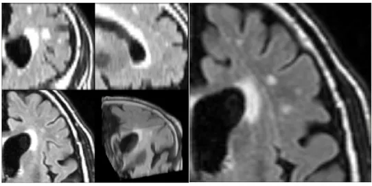
and white matter show a low contrast between them, lesions of the white matter presented as spot of hyperintensity are evident. While the aetiology of these marks is still debated and can be ascribed to multiple factor like massive axon demyelination, ischemic damage, hypoxia, reduced glial presence, there are strong epidemiological associations with conditions such as vascular dementia, vascular cognitive impairment and small vessel disease. Standard clinical grading of these injuries is based on their shape, extension and location, characteristics which are synthesized with a single score (Fazekas Score)[29]. In Figure 3 are reported two examples of T2 Flair showing low grade WMH and severe WMH in two different patients.
14
Figure 3 – Example of T2 Flair images with segmented WMH (in green) and lesions of other nature (Red). Top row: scan of a patient with a low grade WMH (Fazekas 1); Middle row: scan of a patient
15
Given the wide spectrum of disorders associated with White Matter Hyperintensities (WMH), it would be of utmost importance have a repeatable and objective measurement of the lesions, to better stratify the population and use the lesion volume as a proper damage biomarker.
To this aim, we will leverage the Deep Learning technologies to perform automated segmentation of T2-FLAIR brain scans to extract an absolute quantification of WMH. To do this, we will leverage a dataset collected for MICCAI 2017 – White Matter Hyperintensity Segmentation Challenge.
2.3 Methods
2.3.1 Dataset Characteristics
The MICCAI 2017 WMH Segmentation Challenge dataset is composed of brain scans of 60 patients obtained on 3 different scanners from different vendors, 20 for each scanner. Every patient has both 3D-T1 weighted and T2-FLAIR images hand labelled for WMH and different lesions[30]. Lesions have been segmented according to the standard procedures identified in the STRIVE (STandards for ReportIng Vascular changes on nEuroimaging). FLAIR images were acquired according to three different protocols, depending on the clinical unit and scanner vendor:
- UMC Utrecht – 3T Philips - 2D FLAIR sequence (48 transversal slices, voxel size: 0.96×0.95×3.00 mm3, TR/TE/TI: 11000/125/2800 ms)
- NUHS Singapore – 3T Siemens - 2D FLAIR sequence (transversal slices, voxel size: 1.0×1.0x3.00 mm3, TR/TE/TI: 9000/82/2500 ms)
- VU Amsterdam – 3T GE - 3D FLAIR sequence (132 saggital slices, voxel size: 0.98×0.98×1.2 mm3, TR/TE/TI: 8000/126/2340)
3D FLAIR images were reoriented to transversal orientation and resampled to a slice thickness of 3.00 mm, according to the 2D FLAIR specifications.
The images were pre-processed for bias correction by the dataset curators using SPM 12 and the T1 image was co-registered to the T2-FLAIR with elastix.
16
2.3.2 Brain Extraction
In T2 FLAIR imaging the WMH appears as bright spot in the middle of grey appearing white and grey matter, making possible to highlight the lesions. Skull surrounding skin however appear as bright as WMH, making hard to distinguish it from the lesions, especially in slices comprising almost only skin. Thus, to avoid this confounding element we extracted the brain to eliminate all the tissues not useful to learn the characteristic patterns of WMH lesions. To do so, we leveraged the widely used Brain Extraction Tool, part of one of the main neuroimaging analysis suite (FSL). In all the subsequent steps of the pipeline were all executed on masked images, as in Figure 4. All brain extraction results were quality checked to ensure a correct brain segmentation and to ensure that all the WMH lesions were inside the extracted region.
2.3.3 Framework
All the experiments were implemented in Python 3.6, leveraging the Tensorflow (1.13) libraries with Keras (2.3.6) functional APIs, installed on a workstation with Ubuntu 18.06 OS. The workstation was equipped with an Intel 9980XE, 64GB of RAM and a Nvidia Titan RTX, built with 576 Tensor Cores and 24GB of GDDR6 RAM.
Figure 4 – Left: T2 Flair showing similar intensity between WMH and skin. Right: mask of the extracted brain in red, with WMH segmentation in green.
17
On top of this setup, all the experiments were implemented leveraging MisCNN, a framework designed for medical image segmentation. In Figure 5 is depicted the schematics of the framework implementations, with a series of tool to load the neuroimaging data (Nifti I/O interface), preprocess data (normalization, patch extraction, one hot encoding), data augmentation (flips, rototranslation), built-in models and the possibility to expand the library with custom designed models, training and evaluation validation. Some minor implementation have been performed to modify the framework to implement functionalities as 2D patch extraction from 3D volumes.
2.3.4 Preliminary Experiments
In order to leverage three-dimensional shape information provided by volumetric scans of the brain, we first implemented a 3D segmentation network. The experiments were carried on 3D patches extracted from the whole volume and applied a 3D implementation of the networks discussed in 2.3.6. The results were discouraging, with Dice Scores for the WMH segmentations in the order of 0.1. Our hypothesis is that the anisotropy of the images (1x1x3 mm approximatively for the three different scanners) does not add significant information to the segmenting network while the 3D structure has a significantly increased number of weights to train, resulting in a more complex
18
training process. In Figure 6 is shown the loss trend of the best-performing 3D segmentation network.
Thus, we focused the subsequent experiments on the segmentation of planar patches extracted on the X-Y plane. In Figure 7 we can see an example of 3D patch used in preliminary experiments and an example of patch used in subsequent experiments.
2.3.5 Network Architectures
To tackle the problems of medical images semantic segmentation the most common approach has been U-Net and variations, since its first implementation in 2015[31]. The basic principle of U-Net is to structure a network coupling one encoder or convolutional arm which acting as feature extractor and a decoder or deconvolutional arm which leverages the extracted features to provide a dense segmentation of the input image. In this experiment we are implementing two different variations of this
19
architecture, previously published in the context of semantic segmentation[32]: Unet3 and FractalNet.
U-Net3is a extension of the original architecture with focus on the training with a reduced number of samples. The contracting path is a typical convolutional network architecture, with a sequence of two 5x5 convolutions followed by a ReLU and a 2x2 max pooling with stride of 2 to perform down-sampling. After this down-sampling the features are doubled. The expansive path is made of up-sampling blocks followed by a 2x2 up-convolution, halving the features and performing a concatenation with the
Figure 8 – U-NET standard architecture
20
corresponding feature map obtained from the contractile path. The output of this layer is followed by to 5x5 convolutions and a ReLU. The output layer of the network maps the final feature vector to the output number of classes. This architecture extends the original UNet by adding a batch normalization after every ReLU activation function, after each max-pooling and up-sampling layer.
FractalNet is an architecture introduced by Larsson et al. [33]. This networks aims at exploit at a convolutional layer features from different visual levels, joining them to enhance the discriminative capabilities of the network. To this aim, let define C as the index of a truncated fractal fC(·) and the base case of this fractal defined as a single
convolutional layer: f1(z) = conv(z). Defining the expansion rule as:
𝑧′ = 𝑐𝑜𝑛𝑣(𝑧) 𝑓𝐶+1(𝑧) = 𝑐𝑜𝑛𝑣(𝑐𝑜𝑛𝑣(𝑧′) ⊕ 𝑓
𝐶(𝑧′))
It can be defined recursively for successive fractals, with ⊕ as a generic join operation and conv(·) as the convolution operator. The ⊕ operation can be summation, maximization or concatenation, as in this specific architecture. In order to enlarge the receptive field and enclose more contextual information, down-sampling and up-sampling operations are added in the above expansion rule. In particular, a max pooling with a stride of 2 and a deconvolution also with a stride of 2 are added. After the down-sampling operation, the receptive field of a fractal becomes broader. When combining different receptive fields through the join operation, the network can harness multi-scale visual cues and promote itself in discriminating.
2.3.6 Training
Data Augmentation was carried on in order to increase the number of training samples, adding them by applying a combination of transforms to the original dataset. In this case, we applied 3 cycles of data augmentation applying mirroring, rotations and scaling to the original images. Data augmentation is applied at image level, not to the sliced patches. Mirroring was enabled on every image axis, rotations were constrained in a random angle between -15 and +15 degrees, random scaling was applied between 0.85 and 1.25.
21
Training was performed with in batches, with batch size of 128 patches. Networks weights were initialized with a normal distribution for the bias and a glorot normal function for the weights[34]. Three different loss were tested in this experiment: the soft Dice coefficient loss, calculated as one minus the average dice coefficient of each segmented class in a multiclass problem; the soft Dice loss + the categorical crossentropy loss; the Tversky loss, with alpha and beta coefficients = 0.5, which is a loss function for multiclass segmentation with fully convolutional deep networks [35]. The optimization of the weights have been performed with an Adam optimizer [36], with a learning rate of 0.01, β1 = 0.9 and β2=0.999. The training process was repeated for 200 epochs, with a reduction of a ten factor in learning rate after 30 epochs without loss improvement. All experiments were performed with a 5-fold cross validation.
2.3.7 Evaluation Metrics
The evaluation of results was carried on according to the metrics considered in the WMH Segmentation Challenge, using the provided script. The five considered metrics were:
• Dice Score, calculated as 𝐷𝑆 = 1 − 𝑑𝑖𝑐𝑒 𝑑𝑖𝑠𝑠𝑖𝑚𝑖𝑙𝑎𝑟𝑖𝑡𝑦, with dice dissimilarity defined in scipy package
• Hausdorff Distance, 95th percentile, defined as the greatest distance from a
point of one set from the closest point in another set. This parameter is calculated between the segmented lesions and ground truth boundaries. • Average volume difference, expressed in absolute value percentage.
• Sensitivity for individual lesion, defined as the number of detected lesions divided by the number of true lesions.
• F1-score for individual lesion, defined as 2 ∗ 𝑝𝑟𝑒𝑐𝑖𝑠𝑖𝑜𝑛∗𝑟𝑒𝑐𝑎𝑙𝑙
𝑝𝑟𝑒𝑐𝑖𝑠𝑖𝑜𝑛+𝑟𝑒𝑐𝑎𝑙𝑙, with both
precision and recall parameters calculated on the number of identified connected components in the results.
22
2.4 Results
2.4.1 Raw Data
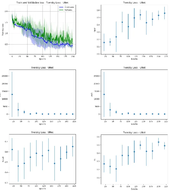
Our first experiment was carried on raw data, which underwent only the brain extraction procedure. We compared the two different architectures presented in 2.3.5 trained with the losses discussed in 2.3.6. The discrepancy between the loss metric evaluated on the sliced patch extracted from the samples and the parameters for the global evaluation of the system shown in 2.3.7, we decided to save a checkpoint of the trained model every 20 epochs of training, to analyze how the evaluation metrics on the whole sample behaved respect to the loss calculated on the patches extracted from the sample. This analysis revealed that all the metrics show a concordant trend with the patch-based loss measured during the validation phase, with an example shown in Figure 9. We can show that the best model in the validation phase corresponds to optimal results in the image-based validation.
23
All the combinations of architectures and losses in this setting show non optimal results. To further enhance the predictive performances of the models and improve the generalization capability of the system we proposed to leverage an ensemble of networks, by combining the predictions of the 5 models obtained in the 5-fold validation, proposing the final result as the average of the 5 outcomes. In Table 1 we report the obtained results and we evaluate the performance of our system in the
24
ranking of the WMH segmentation challenge, assuming that the system will be able to generalize the segmentation process to images obtained by different scanners.
25
Table 1 - Results for Raw Data
2.4.2 Normalized Data
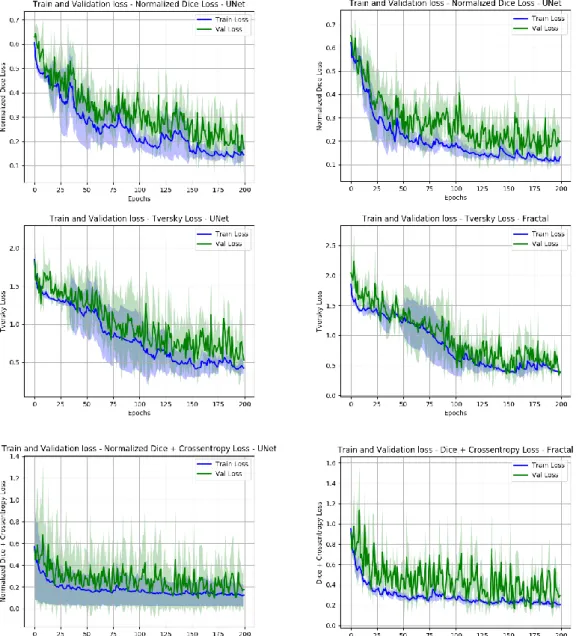
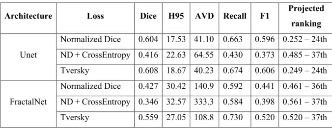
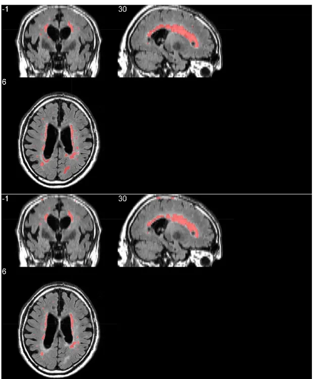
To improve the segmentation performances of the system we implemented a basic preprocessing strategy, the data normalization. As implemented by MIScnn framework normalization is carried on the whole image, before splitting it up in patches. The performances of all the networks greatly improved with this strategy, as shown in Table 2 and Figure 11. In Figure 12 and Figure 13 we show respectively a comparison of all the networks results against the ground truth and the segmentation obtained with the model with the best projected ranking.
Table 2 - Results for Normalized Data
Architecture Loss Dice H95 AVD Recall F1 Projected
ranking Unet Normalized Dice 0.604 17.53 41.10 0.663 0.596 0.252 – 24th ND + CrossEntropy 0.416 22.63 64.55 0.430 0.373 0.485 – 37th Tversky 0.608 18.67 40.23 0.674 0.606 0.249 – 24th FractalNet Normalized Dice 0.427 30.42 140.9 0.592 0.441 0.461 – 36th ND + CrossEntropy 0.346 32.57 333.3 0.584 0.398 0.561 – 37th Tversky 0.559 27.05 108.8 0.730 0.520 0.520 – 37th
Architecture Loss Dice H95 AVD Recall F1 Projected
ranking Unet Normalized Dice 0.755 14.33 29.52 0.729 0.618 0.155 – 20th ND + CrossEntropy 0.738 9.878 27.85 0.599 0.647 0.175 – 22nd Tversky 0.754 14.78 29.60 0.693 0.611 0.171 – 22nd FractalNet Normalized Dice 0.779 10.51 21.70 0.763 0.693 0.096 – 13th ND + CrossEntropy 0.745 17.40 42.03 0.802 0.600 0.157 – 22nd Tversky 0.780 14.21 22.96 0.777 0.658 0.118 – 18th
26
27
2.5 Discussion
With this work we designed an end to end system to segment white matter hyperintensities in T2-FLAIR imaging leveraging fully convolutional networks. The segmentations evaluation describe a system which is capable of achieving a performing score in terms of dice similarity coefficient and average volume difference
28
percentage, while suffering from a low F1-score calculated on the single lesions. This parameter in particular is suggesting the tendency of the network to segment as WMH lesions areas originally labelled as other lesions. Moreover, a visual inspection of the segmentation suggested us that our models show a tendency to underestimate the
Figure 13 - Triplane comparison between ground truth (top row) and segmentation results of our proposed system (bottom row)
29
lesions, as shown in Figure 12 and Figure 13, where smaller isolated lesions are not recognized and where bigger lesions have smaller boundaries. To improve this issue we are currently implementing WMH segmentation leveraging multimodal imaging, to enhance the discrimination between WMH and other lesions using also T1-weighted images, where other lesions have other distinctive patterns to identify them.
Observing the loss per epoch in Figure 11 we can notice the very stable trend showed by Normalized Dice + Crossentropy loss, which reaches the plateau of learning very early in the process, without significant improvements till the end. This suggest us that this is the best performance we could obtain with this combination of loss and network. The Tversky loss showed a better learning trend, while more unstable across different folds. However, the best results and the best projected ranking was achieved by Dice Normalized Loss. This experiment showed the most stable learning trend and reached the best F1- score on the single lesions, the most impacting evaluation on the projected rankings of our networks. The future works will be focused on this combination of architecture and loss: the first step will be the inclusion of a second channel on the contractile path to take into account also the T1-weighted images, other works will be directed to add preprocessing steps to enhance the quality of T2-FLAIR images. Preliminary results have been obtained with image histogram equalization, with drastic improvements on some images showing contracted histograms, while no impact or performance degradation on images with well-distributed histograms.
Finally, it is ongoing the building of the official evaluation docker to test in real field the proposed architectures and obtain an objective ranking in the WMH segmentation challenge.
30
CHAPTER 3. H
YPERTENSIVE PATIENTS
AND EARLY BRAIN DAMAGE
:
A
STRUCTURAL AND FUNCTIONAL
CONNECTIVITY CHARACTERIZATION
3.1 Introduction
The WMH segmentation is a fundamental task to obtain a quantification of the white matter lesion burden, being a representative marker of brain injury associated to ongoing cognitive decline and later-stage hypertension. Thus, it’s nature of established damage phenotype make it useful to stage the degree the pathology, not a good candidate to be a predictive biomarker of early brain damage and vascular cognitive impairment.
To that aim, in our work we looked for alternate parameters to be assessed on hypertensive patients in a early stage of brain damage, in which no damage is diagnosed by a routine clinical MRI exam. We designed a prospective study in which this class of patients, recruited in our outpatient facility at I.R.C.C.S. Neuromed, underwent standard clinical assessments, echocardiography, cognitive assessment and advanced neuroimaging.
31
3.1.1 Patient Sample
To stage the hypertensive disease, we subjected patients to standard organ damage assessment for hypertension target organs, such as vasculature, heart and kidneys. In Figure 14 it is shown the flowchart of the enrolment process of the study, with the main inclusion criteria and the breakdown of excluded patients. The hypertensive population show a hypertrophic cardiac remodelling, characterized by the thickening of heart walls, without loss of function, evidenced by the Ejection Fraction. This suggests a process of adaptive remodelling of the heart, excluding heart failure. No significant vasculature remodelling is evidenced, as shown by the Intima-Media Thickness (IMT) of the carotids. It is worth noting the absence of atherosclerotic plaques in the carotid tract, which could independently contribute to cognitive impairment. Renal function is still unaltered in hypertensive patients, excluding chronic kidney disease (Table 3). The chosen sample represent a homogeneous sample with early damages in organs target of chronic elevated BP levels and no failure in any of those organs. Thus, is a candidate population to explore whether hypertension exerts
32
a damage on the brain and how we can assess it in an early stage, when no sign of WMH or structural damage is present.
Sample Characteristics Normotensive n= 18 Hypertensive n=19 p value Demographic Age. mean (SD) 52 (8) 55 (7) 0.256 Sex. number of females (percentage) 10 (55.55%) 10 (52.63 %) 0.863 Smokers. number (percentage) 3 (16.66%) 4 (21.05%) 0.742 BMI. mean (SD) 25.38 (4.76) 29.96 (4.50) **<0.01
Blood Pressure
Systolic Blood Pressure - mmHg mean (SD) 123 (9.19) 138 (10.97) ***<0.001 Diastolic Blood Pressure - mmHg mean (SD) 77 (6.24) 87 (9.71) ***<0.001
Cardiac Remodeling
LV end-diastolic diameter - mm. mean (SD) 4.85 (0.30) 4.96 (0.33) 0.257 IV septal thickness- mm. mean (SD) 0.91 (0.12) 1.16 (0.14) ***<0.001 LV posterior wall thickness- mm. mean (SD) 0.91 (0.14) 1.09 (0.09) ***<0.001 LV mass index (LVMI2.7) - g/m2. mean (SD) 37.69 (9.11) 54.66 (8.28) ***<0.001
Relative wall thickness - RWT. mean (SD) 0.37 (0.05) 0.44 (0.04) ***<0.001 Diastolic dysfunction (percentage) 4 (22.22%) 15 (78.94%) ***<0.001 LV Ejection fraction - %. mean (SD) 65.44 (6.20) 68.63 (7.03) 0.153
Carotid Artery (CA) Thickening Internal CA (right) - IMT. mean (SD) 0.76 (0.18) 0.86 (0.23) 0.137 Common CA (right) - IMT. mean (SD) 0.80 (0.14) 0.87 (0.13) 0.118 Internal CA (left) - IMT. mean (SD) 0.76 (0.17) 0.87 (0.21) 0.082 Common CA (left) - IMT. mean (SD) 0.81 (0.13) 0.90 (0.18) 0.094
Renal damage
Creatinine - mg/dL. mean (SD) 0.75 (0.17) 0.74 (0.15) 0.848 Microalbuminuria - mg/24hrs. mean (SD) 11.84 (16.08) 17.30 (17.96) 0.338 Estimated GFR – mL/min. mean (SD) 114.84 (34.95) 127.12 (41.50) 0.338
33
Cognitive tests revealed that hypertensive population show a significantly reduced MoCA score (Montreal Cognitive Assessment, the gold standard for vascular cognitive impairment diagnosis) (Table 4)[37]. The damage is focused on executive function, as can be seen in Table 5 in which are reported the values obtained in different subscales of MoCA test, to better differentiate the cognitive domains with impaired function. Normotensive n= 18 Hypertensive n=19 p value Cognitive Assessment
IADL – score. mean (SD) 7.7 (0.75) 7.7 (0.65) 0.950 MoCA – score, mean (SD) 26.00 (2.43) 22.36 (2.73) ***<0.001
Semantic Verbal Fluency – score. mean (SD) 48.67 (11.44) 43.68 (12.24) 0.210 Paired-Associate Learning – score. mean (SD) 13.92 (4.04) 9.55 (5.31) **<0.01 Stroop Color Word Test – score. mean (SD) 0.22 (0.65) 0.97 (1.51) 0.059 Stroop Interference Test – time. mean (SD) 16.68 (7.90) 25.99 (12.11) **<0.009
Table 4 - Cognitive Assessment Normotensive
n= 18 Hypertensive n=19 p value MoCA cognitive subdomains
Visuospatial – score. mean (SD) 3.2 (1) 3.35 (1) 0.680 Executive Functions – score, mean (SD) 3.6 (0.7) 2.4 (1.2) **<0.01 Language – score. mean (SD) 5.3 (0.8) 4.9 (0.7) 0.216 Attention – score. mean (SD) 5.2 (1.3) 4.7 (1.5) 0.324 Memory – score. mean (SD) 2.9 (1.7) 1.4 (1.3) **<0.01
Table 5 - MoCA cognitive subdomains
3.2 Structural
Connectivity:
Diffusion
Tensor
Imaging applied to Hypertensive Patients
Our first aim in this study was to characterize the microstructural damage that hypertension exerts on cerebral white matter, the region of the brain which connects
34
different areas of the cerebral cortex between them and with the subcortical structures. Damages to this region have classically been associated and diagnosed with the WMH, lacking methods to investigate its integrity in early stages of damage. To this aim, the use of Diffusion Tensor Imaging (DTI) is a powerful tool. Briefly, by analysing the Brownian motion of the water in the brains we can reconstruct a model of the neuronal fibers, thus evidencing the connections existing in the brains and their microstructural properties[38, 39]. (see Appendix A – MRI Sequences for more insights)
3.2.1 Diffusion parameters
To fully characterize the diffusion at each voxel the first measure extracted is the
Mean Diffusivity (MD), which is the sum of the diagonal elements of D, is a measure
of the magnitude of diffusion and is a rotationally invariant measure[40]. From MD we can thereby extract the most widely used measure of anisotropy, the Fractional
Anisotropy (FA) [40].
𝐹𝐴 = √(𝜆1− 𝑀𝐷)
2+ (𝜆
2− 𝑀𝐷)2+ (𝜆3− 𝑀𝐷)2
35
Note that the diffusion anisotropy does not describe the full tensor shape or distribution. This is because different eigenvalue combinations can generate the same values of FA. Although FA is likely to be adequate for many applications and appears to be quite sensitive to a broad spectrum of pathological conditions, the full tensor shape cannot be simply described using a single scalar measure. However, the tensor shape can be described completely using a combination of spherical, linear and planar shape measures. The last two measures are secondary combination or amplitude evaluation of the eigenvalue: the Axial Diffusivity (AD) [40], which is the greatest eigenvalue (λ1) and the Radial Diffusivity (RD) [40] which is the average of the others
36 eigenvalues (𝜆2+𝜆3
2 ). An example of the maps is shown in Figure 15. The scalar maps
can’t represent the principal directions of the diffusion. A standard color coding, superimposed to an FA map, has been vastly used to represent the principal eigenvector in each voxel (Figure 16). The green represents diffusion on the Posterior-Anterior direction, red represents diffusion on the Left-Right direction, blue represents diffusion on the Upper-Lower direction.
Every parameter’s alteration can be associated to a specific type of damage of the analysed area: FA and MD are associated with primary axon degeneration. Lower FA values indicate disorganized fibers, which are affected by microstructural processes such as demyelination, axonal degradation, or gliosis. Of the two, MD, is a more
37
sensitive measure even though it is less specific, and its results can be increased by any pathological process affecting the neuronal cell membranes. Incremental variations in RD are associated with myelin breakdown, whereas in AD describe secondary axon degeneration.
3.2.2 From tensorial model to probabilistic diffusion
modelling
The main limitation of DTI deterministic methods can be found in the simplistic modelling of a single fiber per voxel. White matter fibers are microscopical structures and brain networks are intricate and it is often needed the connection between distant areas. The typical spatial resolution of a MRI dataset is 1x1x1 mm, so one voxel is very likely to contain more than a bundle of fiber. To overcome this limitation a probabilistic approach has been developed to model the crossing fibers in each voxel: BEDPOSTX (Bayesian Estimation of Diffusion Parameters Obtained using Sampling Techniques. X stands for Crossing Fibers)[41]. This technique exploits the partial volume model (also called ball and stick model) which assumes that a fraction of diffusion is along a single dominant direction, and that the remainder is isotropic. The algorithm also estimates how many fibers can be modelled in each voxel of the space, creating a multi-fiber distribution parameter estimation. The output of BEDPOSTX is a series of scalar maps per estimated fiber. For each fiber we have the estimates of theta, phi (polar coordinates identifying the main diffusion direction) and anisotropic volume fraction. These maps are necessary to perform probabilistic tractography. The information from multiple fibers can be superimposed to have a global view of the modelled fibers distribution. In Figure 17 the modelling of the first fiber, in red, the second fiber, in blue, and their superimposition is shown. In detail the zoom of the green rectangle: it’s possible to see how, in high anisotropy regions, the models are mixed and the two fibers point out different diffusion directions.
38
3.2.3 Probabilistic tractography
After the multiple fibers modelling, classical tractography methods are unfeasible. Having no longer a single principal direction to follow means that a deterministic tractography algorithm is not able to decide which fiber a streamline should follow. To solve this issue, PROBTRACKX (Probabilistic tracking with crossing fibres) has been introduced[42]. To perform probabilistic tractography we need to define a seed voxel (or a group of seed voxels) and a target voxel (or a group of target voxels). This method repetitively samples starting at the seed voxels from the distributions of voxel-wise principal diffusion directions, each time computing a streamline through these local samples to generate a probabilistic streamline or a sample from the distribution
39
on the location of the true streamline. By taking many such samples PROBTRACKX is able to build up the histogram of the posterior distribution on the streamline location or the connectivity distribution between the seed region and the target region. In Figure 18 the spatial histogram of the connectivity distribution of anterior thalamic radiation tract is shown. The colour scheme represents the confidence of the connection: yellow stands for a high connectivity region, red stands for a low connectivity region.
3.2.4 Analysis Pipeline
In order to process data collected from the study and make them comparable, it has been necessary to develop and implement a rigorous analysis pipeline. The stages of this workflow are here presented and discussed (Figure 19).
40
First, structural and DWI images are examined by an expert radiologist to exclude pathologies which could affect the outcome of the study (gliosis, white matter hyper intensities, ischemia). After the radiological response the raw DWI data begins the processing with BET (Brain Extraction Tool)[43], a tool which deletes from the image all non-brain tissues and creates a binary mask to identify the brain. The images so obtained are then processed with the eddy current correction tool[44]. Eddy currents are characteristics parasite currents induced by the magnetic field, resulting in image artefacts like shading and blurring. Corrected images are then co-registered to a common atlas in a standard space. On the resulting image is fitted the tensorial model, to obtain the standard parameter maps, then BEDPOSTX is performed in order to produce data for tractography[41].
Preprocessing
• Radiological Assessment • Brain Extraction • Eddy Current Correction • Tensor Model Fitting • BEDPOSTX
Probabilistic
Tractography
• PROBTRACKX • Tract Quality Check
Parameters
Extraction
•Mean FA per tract •Mean MD per tract •Mean RD per tract •Mean AD per tract •Volume per tract
41
The second stage of the pipeline is the tractographic analysis. In this step we create a per subject segmentation of the white matter based on connectivity features[45]. The main tract of the white matter has been characterized by a team of expert neuroanatomists[46]. In order to perform the segmentation, each tract has been described with a series of binary masks in standard space: the seed mask, the region from which the tract is originated; the target mask, the region where the tract is headed to; the stop mask, a region which describes a terminator for streamlines; the exclusion
mask, if streamlines crosses this region are eliminated from the model. PROBTRACK
is performed tract by tract to obtain a connectivity distribution for every tract specified in the protocol[42]. After that the tracts are thresholded to optimize the repeatability of the parameters’ extraction. A different threshold is used for visualization. Tracts are identified by their functionality: in Figure 20A the right hemisphere (RH) fraction of the callosal tracts is shown, in Figure 20B the RH of the limbic system tracts is shown, in Figure 20C the RH of the associative tracts is shown, in Figure 20D the RH of the projection tracts is shown. On a per patient basis a visual inspection and tract quality check is performed, to exclude from the study potential outliers (interrupted tracts, errors due to misaligning of masks and anatomic structures). Once we have obtained the white matter segmentation for the patient, we proceed to extract the diffusion parameters associated with each tract. After a co-registration of segmentation maps and parameters maps, segmented areas are used as ROI in which the diffusion parameters are averaged and extracted. For each tract, volume is also calculated in order to exclude tract atrophy. After the clinic study the first data analysis approach has been the univariate statistical comparison, to explore where the hypertension could have caused damages and how was this damage characterized.
42
3.3 Functional Connectivity: resting state functional
MRI applied to Hypertensive Patients
Our second aim in this study was to characterize not only the damage that hypertension exerted on the brain structure, but which was the consequent functional damage. While mainly limited to psychiatric or neurodegenerative disorders, resting
43
state functional MRI is a potent tool to assess the functional organization of the brain. By acquiring the blood-oxygen-level dependent signal (BOLD signal) we can image the relative concentration of oxygenated and deoxygenated blood in each voxel, and sampling this signal repeatedly let us reconstruct the regional neuronal activations[47]. (see Appendix A – MRI Sequences for more insights)
3.3.1 Functional Network Analysis
It has been extensively demonstrated that in normal subjects the brain in resting state shows a consistent pattern of synchronous alterations. Since the first works using this technique in small populations of healthy controls, it was very evident the activation during rest time of an ensemble of regions which were conversely negatively associated and non active during every kind of task previously administered: the Default Mode Network (DMN)[48-50].
Subsequent efforts were aimed at resolving all the synchronous connections through different regions of the brains, and these efforts resulted in precise mapping of each brain region associated to a group of synchronous activations dedicated to generic type of brain activity. One of the pivotal works in rs-fMRI research mapped 7
44
coarse networks of activation which could be eventually divided in 17 fine networks, each one consistent between one thousand subjects included in the study. To do this, Yeo at al. applied a clustering algorithm to group the voxels taking into account both their functional time course and their distance and regional profile[51].
45
Other approaches were able to extrapolate functional networks from the raw data: Independent Component Analysis (ICA) is one of the main tools exploited in functional MRI analysis[52]. ICA is used to find a set of statistically independent maps (which are the maps depicting the regions of the functional networks) with time courses associated between them (which is the measure of their functional connectivity). This technique let us extrapolate the spatial and temporal information of the brain networks from the data, without any a-priori knowledge, and without any a-priori constraint. Usually the results of ICA, while explaining the quasi-totality of the starting dataset, need to be cleaned to rule out the spurious signals from regions not involved in functional connectivity (such as CSF or, in a classical vision of the problem, white matter). Once obtained the regional maps and their associated time course, we can proceed with the analysis of functional connectivity between different
46
patient populations. It can be considered intra network connectivity (the differences between FC in the synchronicity between different regions of the same network) or inter network connectivity (the differences between FC in the synchronicity of different regions between different networks). In Figure 23 it’s shown an example of a full connectome ring, in which every connection is represented in a round scheme, color coded by intensity of the correlation and grouped by the functional network of origin.
3.3.2 Graph Analysis
Once we evaluate the correlation between the timeseries of different regions, it is possible to build an undirected graph of connections. The resulting graph will be composed of a node for each region and edges between region whom timeseries correlation is above a certain threshold value[53].
On this built graph we can estimate topological measurements for each node and we can aggregate them across the network[54]:
• Degree: the degree of a node is the number of edges associated to the node, and estimates the network centrality and local connectivity of a node • Average Path Length: Average length of the paths connecting a node with
each other node in the network, gives an estimate of the compactness • Clustering Coefficient: Fraction of edges among all possible edges in the
local neighbouring sub-graph for each node. It is an estimate of the interconnectedness in sub-graphs, often measures the small-world characteristics of a network.
• Global and Local Efficiency: Average of inverse-distances between each node and all other nodes in the graph. The global efficiency measures the centrality of a node in a network, while the local efficiency is the same metric applied to neighbouring sub-graphs.
• Betweenness Centrality: Measure of node centrality in a graph, measures the percentage of optimal paths between other nodes in which the node is included.