Two phase microfluidics: new trend in model identification

F

DOTTORATO DI RICERCA IN INGEGNERIA ELETTRONICA,

AUTOMATICA E DEL CONTROLLO DI SISTEMI COMPLESSI

XXIVBATCH

PRINCIA ANANDAN

T

WO PHASE MICROFLUIDICS

:

N

EW TREND IN MODEL IDENTIFICATION

PH.D.THESIS

TUTOR:PROF.M.BUCOLO

CO-ORDINATOR:PROF.L.FORTUNA

I

The aim of the research is to give a proper understanding of the physical aspects involved in two-phase microfluidic systems: from the theoretical point of view to the development of numerical solutions for the flow field by Computational Modeling (CM) issue studies devoted to standard droplet generator for separation and segmented flow, bubble and drop formation, breakup and coalescence and then with increasing complexity in large scale microfluidic processors, bubble logic i.e. bubble to bubble hydrodynamic interaction provides an on-chip process control mechanism integrating chemistry and computation. This concept has been implemented using

COMSOL multiphysics 3.5a software. These show the non-linearity, gain,

bistability and programmability required for scalable universal computation. Alongside experimental work, numerical tools, such as computational fluid dynamics (CFD), allow us to study and analyses the behavior of immiscible fluids within microchannels. Good understanding of these microfluidic flows provides us with leverage when utilized in chemical and biological applications. The study in the context of micro-optofluidics analysis have allowed to define in some detail the integrated system used to Thorlabs has provided for the experiments in micro-optofluidics. In particular, the characterization of the microfluidic detection devices has been used in the experimental studies of two-phase flow. In addition, the analysis carried out in the various micro-channels fixed unique features in terms of flow rates for each dimensions. The key issue is finally the study and designs of an embedded system optofluidics in micro-optics Lab-On-Chip (LOC), which allows achieving very narrow spaces in a microfluidic system, ensuring a degree of portability, which it integrates optical realizing therefore, the right balance between the two disciplines. Played as part of a global project in which design and manufacture of micro devices LOC, and experimental studies within micro-optofluidics could easily fit in a biochemical analysis of the microscopic scale of biological particles of various kinds. The dynamical

II

microfluidic Two-Phase Flow process is presented. The experimental time series are used to synchronize another system with known mathematical model but unknown parameters: the Chua’s oscillator. This system has been chosen for its simple mathematical structure and for the Possibility, respect to other chaotic systems, of mapping various non-linear experimental phenomena. A genetic algorithm was exploited for parameters estimation in relation to an optimization index that takes into an account of synchronization of master (microfluidic system) and slave system (Chua’s oscillator).

III

During these years at University of Catania, I met a lot of persons, wonderful persons I would say! I would like to thank all of them for making me feeling so comfortable with their kindness. I have really felt like in a big family.

First and foremost I would like to express my sincere gratitude to my supervisor Ms. Maide Bucolo, who gave me not only her scientific and technical support, which was great, but especially her friendship. She has taken the time to teach me a great deal about the field of fluid mechanics by sharing with me the joy of modernism in research. She took good care of me. Even though I have many shortcomings, she always tried to understand my situation and guide me. She has been kind enough to share her knowledge not only about academics, but also other important things in life. It is my greatest fortune through all my life to meet her. Wish to say thank you, deep in my heart, for so many lives, you're a big part.

I would like to thank the gentlemen who have generously served and supported President. Dr Luigi Fortuna. It is a great tribute to meet such a person in my life.

I thank Ms. Florinda Schembri my colleague for her kind co-operation and encouragement in my academic year.

I would like to thank also my generous roommate Alessandra Politini for the nice time we have spent together.When I needed help, you were always there, my issues and problems I knew I could share. I truly appreciate that you are my friend. I will treasure all the good and bad moments we shared together. And to all my Indian, Italian, Egyptian, and my foreign friends, especially Mina Halim and Mina Elia who have provided light relief making the PhD process bearable!

I want to express my utmost thanks to my family, dad, mom and my bro. Without their solid support and consistent courage, it would not have been possible.

ABSTRACT _I

INTRODUCTION _i

CHAPTER-1 COMPUTATIONAL MODELING IN TWO PHASE FLOW MICROFLUIDICS

1.1 Theoretical Background of Microfluidic Two Phase Flow ₃

1.1.1 Continuity Equation ₄

1.1.2 Navier Stokes Equation ₅

1.1.3 Energy Equation ₉

1.1.4 Dimensional Number in Microfluidics ₉

1.2 Two Phase Microfluidics ₁₈

1.3 Computational Fluid Dynamics (CFD) ₂₄

1.3.1 Level set ₂₆

1.3.2 Phase field ₃₂

1.4 Phase Field for Two Phase flow Microfluidics ₃₆

1.5 COMSOL Platform ₃₇

1.6 COMSOL verses other Platforms ₃₉

CHAPTER-2 LIBRARY OF COMPUTATIONAL MODELING FOR MICROFLUIDIC

CIRCUIT DESIGN

2.1 Computational Modeling (CM) Issues ₄₄ 2.1.1 Physical Properties of the fluids ₄₄

2.1.2 Numerical Properties ₄₆

2.1.3 Input Profile ₄₇

2.1.4 Input flow rates ₄₉

2.1.5 Boundary Conditions ₄₉

2.1.6 Sub-domain Settings ₅₂

2.1.7 Chip Geometry ₅₃

2.1.8 Meshing ₅₄

2.2.2 Parametric CM with Long Channel ₆₂ 2.2.3 Flow Pattern Generation ₆₇ 2.2.4 Comparison: water-air versus water-hexadecane ₇₇

2.3 Bubble Logic ₇₉

2.3.1 Computational modeling for the AND/OR Logic Gates-1 ₈₄ 2.3.1.1 Focus on two different type of disperse phase (air

versus Hexadecane) 93

2.3.2 Computational modeling for the AND/OR Logic Gates-2 ₉₅ 2.3.3 Computational modeling for the NOT Logic Gates. ₁₀₁ 2.3.4 Computational modeling for the Memory Circuits. ₁₀₈

CHAPTER-3 OPTICAL ACTUATION AND MONITORING IN MICROFLUIDICS

3.1 Basic Concept of optics for Microfluidics ₁₁₅ 3.1.1. Definitions and Recurrent Parameters ₁₁₆ 3.1.2. The optical phenomena ₁₂₀ 3.2 Methods of Optical Actuation ₁₂₆ 3.2.1 Thermo-Capillary Effect ₁₃₁ 3.3 Method of Optical Monitoring ₁₃₃ 3.4 Examples of Implementation of Optics in Microfluidics ₁₃₇ 3.5 Blocks to design an Electro-Optical System ₁₄₀

3.5.1 Light sources ₁₄₁

3.5.2 Methods for the transport of the image ₁₄₃

3.5.3 Optical Detectors ₁₄₅

3.6 Experimental Optical Workbench ₁₄₇ 3.6.1 Basic Optical Tweezer System (OTKB) ₁₄₇

3.6.2 Customized OTKB ₁₅₃

3.7 Static Characterization of Optical Detection ₁₅₄ 3.7.1 Positioning Photodiodes ₁₅₅ 3.7.2 Terms of Reference Signal ₁₅₆

3.8 Setup of Microfluidic System ₁₆₂ 3.9 Flow Pattern in Microfluidic Chip ₁₆₈ 3.9.1 Straight Channel (320µm) ₁₇₀ 3.9.2 Serpentine Channel (640µm, 320µm) ₁₇₃ 3.10 Y-junction Computational Modeling for Droplet Generation ₁₈₂

3.10.1 Parametric CM ₁₈₂

3.11 Flow Pattern through CMs of Microfluidic Chip ₁₈₄ 3.11.1 Straight Channel (320µm) ₁₈₅ 3.11.2 Serpentine Channel (320µm, 640µm) ₁₈₆

CHAPTER-4 DATA DRIVEN IDENTIFICATION OF BUBBLE FLOW IN

MICROCHANNEL

4.1 Processes Identification in Microfluidics ₁₉₁

4.2 Physical Background ₁₉₅

4.3 Experimental Setup and Time series Analysis ₁₉₆

4.3.1 Nonlinear indicators ₁₉₉

4.4 Two-Phase Flow Modeling ₂₀₁

4.4.1 Synchronization of chaotic systems ₂₀₂

4.4.2 The Chua’s oscillator ₂₀₄

4.5 Genetic Algorithm Optimization Technique ₂₀₅ 4.6 Bubble Flow Non-Linear Models ₂₁₃

CONCLUSION ₂₁₉

i

he earliest microfluidic devices demonstrated that fluidic components could be miniaturized and integrated together, leading to the idea that one could fit an entire “Lab -on-Chip” (LOC), in much the same way that a microelectronic circuit is an entire computer on a chip. Since then, there has been tremendous interest in harnessing the full potential of this approach and, consequently, the development of countless microfluidic devices and fabrication methods.

Elastomeric materials such as Polydimethylsiloxane (PDMS) have emerged recently as excellent alternatives to the silicon and glass used in early devices fabricated by MEMS (micro-electro-mechanical systems) processes. Simplified device fabrication and the possibility of incorporating densely integrated micro valves into designs [44] have helped microfluidics to explode into a ubiquitous technology that has found applications in many diverse fields. This chapter begins with a brief introduction to microfluidics, and the physical background followed by a description of the Computational Modeling for Microfluidic Circuit Design. Alongside experimental work, numerical tools, such as computational fluid dynamics (CFD), allow us to study and analyze the behavior of immiscible fluids within microchannels.

Good understanding of these microfluidic flows provides us with leverage when utilized in chemical and biological applications. Many factors taken together have contributed to the success of this technology, as discussed in the final section. In Chapter 3, these desirable properties are used as a guide for the comparison of experimental microfluidics versus computational modeling to draw a

ii

CFD.

Microfluidics- As numerous investigators have pointed out, scaling

down fluidic processes to the micro scale offers many significant advantages [2, 4, 43, 44, 45, 46, 47], some stemming directly from the reduction in size and others a result of the ability to integrate at this scale.

Benefits of size reduction- One obvious advantage are that

miniaturized components and processes use smaller volumes of fluid, thus leading to reduced reagent consumption. This decreases costs and permits small quantities of precious samples to be stretched further (for example, divided up into a much larger number of screening assays) [2].

Quantities of waste products are also reduced. The low thermal mass and large surface to volume ratio of small components facilitates rapid heat transfer, enabling quick temperature changes and precise temperature control. In exothermic reactions, this feature can help to eliminate the buildup of heat or “hot spots” that could otherwise lead to undesired side reactions or even explosions [5]. The large surface to volume ratio is also an advantage in processes involving support-bound catalysts or enzymes, and in solid-phase synthesis.

At the small length scales of microfluidic devices, diffusive mixing is fast, often increasing the speed and accuracy of reactions. Dramatic performance improvements are often seen in microfluidic assays as well: reduced measurement times, improved sensitivity, higher selectivity, and greater repeatability, are common. For

iii

separations by the rapid dissipation of Joule heat. In some separations, sensitivity is improved simply because the reduced measurement time leads to a lower degree of peak broadening [2, 5].

Microfluidic devices sometimes enable tasks to be accomplished in entirely new ways. For example, fluid temperature can be rapidly cycled by moving the fluid among chip regions with different temperatures rather than heating and cooling the fluid in place. A device to screen for protein crystallization conditions harnesses free-interface diffusion—a process that is practical only at the micro scale—to explore a continuous range of conditions when protein and salt solutions are gradually mixed [4]. The laminar nature of fluid flow in microchannels permits new methods for performing solvent exchange, filtering, and two-phase reactions [42].

Benefits of automation and integration - Many microfluidic

technologies permit the construction of devices containing multiple components with different functionalities. A single integrated chip could perform significant biological or chemical processing from beginning to end, for example the sampling, pre-processing, and measurement involved in an assay.

This is the kind of vision that led to the terms “lab-on-a-chip” and “Micro Total Analysis System (μTAS)”. Performing all fluid handling operations within a single chip saves time, reduces risk of sample loss or contamination, and can eliminate the need for bulky, expensive laboratory robots. Furthermore, operation of microfluidic devices can be fully automated, thus increasing throughput, improving

iv

human error. Automation is also useful in applications requiring remote operation, such as devices performing continuous monitoring of chemical or environmental processes in inaccessible locations. Another way to increase throughput is to exploit parallelism. Single chips have been demonstrated that perform hundreds or thousands of identical assays or reactions [1, 2, 42].

These chips utilize synchronization and control-sharing so that their operation is not significantly more complex than that of a non-parallel chip. They also feature on-chip distribution of a single input sample to thousands of micro reactors—an interesting solution to the micro-to-macro interface problem. This problem refers to the mismatch between sample sizes that can be easily manipulated in the lab (μL–mL) versus the volume of micro reactors (pL–nL).

The task of controlling thousands of individual valves with a much smaller number of off-chip control inputs is achieved by implementing multiplexers or other more complex logic on-chip, as is done in microelectronic chips. Being planar and on the same scale as semiconductor integrated circuits, microfluidic devices are ideally poised to be integrated with electronic or optical components such as sensors, actuators, and control logic.

On the sensing side, significant progress has been made: chemical, electrical, optical absorption, fluorescence, flow, temperature, and pressure sensors are just some examples that have been reported. Numerous actuators, such as valves, pumps, heating elements, and electrodes for electrophoresis or electro kinetic flow, have also been demonstrated. Beebe et al. [16] devised an interesting

v

respond to particular properties of the fluid by swelling and directly actuating a valve. In general, however, the potential of integrated control logic has been largely untapped. In the future, hybrid devices that perform sophisticated in situ monitoring and computation may emerge, perhaps to implement feedback control circuits that maintain optimum operating conditions or detect problems. Small integrated microfluidic devices may also offer the feature of portability, enabling mobile applications in chemical analysis, point-of-care medicine, or forensics.

The ability to perform integrated diagnostic tests where they are needed rather than in a centralized lab could reduce costs, improve turn-around time, and reduce the risk of sample mix-up. If manufactured cheaply, devices could be disposable, eliminating cross-contamination between tests. Microfluidic applications in drug delivery are also possible.

Application areas- The literature contains many thousands of reports

of reactions and assays that have been carried out in microfluidics devices (see reviews in [1, 2, 4, 42, 43, 44, 45, 46, and 47]). Some have shown significant improvements in performance compared with their macro scale counterparts and have successfully competed in the commercial marketplace. In some rare cases, micro scale implementations have completely transformed the way that a certain type of experiment is performed or have enabled massively parallel experiments that previously could not even be contemplated. Among the numerous biological and biochemical processes demonstrated are

vi

screening, cell counting and sorting [84], electro-phoretic separations, nucleic acid extraction, analysis of unpurified blood samples [290], DNA sequencing [2, 4], screens for protein crystallization conditions [97], cell culture studies [2], and single cell manipulation [293]. In chemistry applications, dramatic improvements in synthetic yields and selectivities have been observed [2, 42, 44]. In addition, microfluidic devices may make possible novel reactions or processing conditions by unprecedented control over surface chemistry, local heat and mass transfer [5], or reagent concentrations in space and time (using electro-osmotic flow) [12]. The greater degree of control may help to design experiments to increase knowledge about many chemical processes [2].

Several investigators have also argued that micro reactors could be used in industrial chemical production or waste treatment plants if volumetric processing requirements are low [1, 2, 4, 42, 43, 44, 45, and 47]. Scaling up production can be achieved by bringing additional micro reactors into service at a relatively low incremental cost rather than constructing a new higher-capacity reactor—an ability that would be especially useful in pilot plants or in industries with production demands that change with time or geographical location.

The ability to set up production when and where it is needed could decrease the need for storage and transportation of hazardous or short-lived chemical products. Furthermore, micro reactors have the potential to increase the safety of dangerous processes such as the fluorination of aromatic compounds and the synthesis of organic peroxides from acid chlorides by accurate temperature control and

vii

failure, the consequences will be relatively minor due to the small mass of material present in the reactor at a given time.

Chapter-1

The aim of this chapter is to give a proper understanding of the physical aspects involved in two-phase microfluidic systems: from the theoretical point of view to the development of numerical solutions for the flow field.

3

C

M

T

P

F

M

1.1 Theoretical Background

Microfluidics is defined as continuous where the continuum hypothesis is assumed valid. It states that the macroscopic properties of a fluid is the same as if the fluid were perfectly continuous in structure instead of consisting of molecules. In this case, physics quantities such as the mass, momentum, and energy associated with a small volume of fluid containing a sufficiently large number of molecules are taken as the sum of the corresponding quantities for the molecules in the volume.

The physical properties of the fluid per volume, such as mass density, energy density, force density and momentum density have therefore to be considered. The continuum hypothesis is no longer valid when the system under consideration approaches molecular scale. This happens in Nanofluidics, e.g., in liquid transport through nanopores in cell membranes or in artificially made nano-channels.

Here, you will be exposed to the laws that are the foundation of Microfluidics. The focus is particularly on the Navier-Stokes equations and the conservation of mass, which allow describing the dynamic behavior of fluids in micro-channels [1].

By considering some parameters whose knowledge allows assessing in advance the behavior of the entire system under certain constraints. Will then describe some examples of practical applications, including geometry through which you can get the droplet break-up.

4

1.1.1 Continuity Equation

Under the continuum hypothesis, the Eulerian concept where the physical properties of the fluid are described in terms of fields, focusing on fixed point in space and observing how the fields evolve in time at these points. The first fundamental equation of fluid mechanics is the continuity equation, expressing the conservation of mass in classical mechanics; this is needs to be considered it is compressible or incompressible fluids.

Take in account of material particle of position x(t) and of volume ⋎(t) riding along with the flow. The mass m of the particle can then be expressed as the local density of the fluid times the particle volume m = ρ(x, t) ⋎(t). The rate of change of this quantity is determined from 𝑑 𝑑𝑡 𝜌 𝑥 𝑡 , 𝑡 ⋎ 𝑡 = 𝜕𝜌 𝜕𝑡 ⋎ + ∇𝜌 ∙ 𝑑𝑥 𝑑𝑡 ⋎ + 𝜌 𝑑 ⋎ 𝑑𝑡 = 𝜕𝜌 𝜕𝑡 + ∇ ∙ 𝜌𝜐 (1.1)

where the second equality follows from the definition of the velocity field dx/dt = 𝜐 and the change in particle volume is expressed by the divergence of the velocity field lines d⋎/dt =

(𝛻 ∙ 𝜐) ⋎. Now since the mass of the particle is conserved, thus

arrive at the equation of continuity 𝜕𝜌

𝜕𝑡 + 𝛻 ∙ 𝜌𝜐 = 0. (1.2)

In the first case, density ρ may vary as a function of space and time, while for incompressible fluids ρ is constant in space and time.

5

In many cases, especially in microfluidics, where the flow velocities are much smaller than the sound velocity in a liquid, the fluid can be treated as incompressible [1]. Notice however that the opposite is not true with a divergence free velocity field and a density constant in time the continuity equation only implies that the density is constant along streamlines.

1.1.2 Navier Stokes Equation

The solution of problems involving two immiscible fluids in contact requires the solution of the Navier-Stokes equations containing the contribution of the surface tension, which allows the description of the phenomena of coalescence and / or breakage of the interface separation.

The Navier-Stokes equations are a system of partial differential equation that describes the behavior of a fluid from the macroscopic point of view. The basic hypothesis is that the fluid can be modeled as a continuous body deformable. They assume therefore the continuity of the fluid under examination, i.e. the system loses its validity in the study of a rare gas. The equations owe their name to Claude-Louis Navier and George Gabriel Stokes.

The predictive efficiency of these equations is paid in terms of computational difficulties. In the general case involve a mix of five scalar equations partial differential equations lie 20 variables. The balance between equations and unknowns is with the definition of the properties of the fluid considered, any field strengths into play and mathematical considerations. Furthermore,

6

of their non-linearity, the Navier-Stokes equations do not allow almost never an analytical solution (i.e. an exact solution), but only numeric (an approximate solution with a numerical method).

The Navier-Stokes equations are able to fully describe any fluid flow, also turbulent. In particular for a turbulent flow, that is, where the trajectories of the particles flow are no longer constant over time, a numerical approach of calculation is called general mind direct numerical simulation [2]. Due to the fact that the computing resources necessary for their resolution grows with the Reynolds number and that this number can have values of the order

of 106-109, such an approach is technically impossible. Alternative

to the numerical simulation can be taken less expensive systems such as the formulation injured equations mediated.

The equations are supplemented by boundary conditions and initial conditions (conditions imposed at the beginning time of the phenomenon to be studied). They can also be integrated by the equation of state of an ideal gas and from the equations of conservation of the individual gaseous species in the case of a gas mixture. The solution of equations provides the field of fluid velocity. From this it will be then possible to trace all the other quantities that characterize the flow. To this end it has developed a branch of fluid dynamics called Computational Fluid Dynamics (CFD).

“The Navier-Stokes equations are a system of partial differential equations that describes the behavior of a fluid from the macroscopic point of view. The underlying assumptions of such a system are that the fluid may be understood as a continuous body deformable.” With the term continuous deformable means a

three-7

dimensional body occupying a certain volume that during its motion is subject to deformation is of volume and shape.

The predictive efficiency of these equations is paid in terms of computational difficulties. They also are able to fully describe any fluid flow, also turbulent. In particular for a turbulent flow, that is, where the trajectories of the particles flow are no longer constant over time, a numerical approach of calculation is generally called direct numerical simulation. In the general case involve a mix of five scalar equations partial differential equations in 20 variables. The balance between equations and unknowns occurs with the definition of the properties of the fluid under consideration, any of the field strengths in play and with mathematical considerations.

Because of their non-linearity, the Navier-Stokes equations do not admit almost never an analytical solution (i.e., an exact solution), but only numerically (an approximate solution with a numerical method). The equations are supplemented by boundary conditions and initial conditions. The solution of equations provides the field of fluid velocity. From this it will be then possible to trace all the other quantities that characterize the flow.

Again by considering a material particle riding along with the flow, the particle momentum is then p = m𝜐, with rate of change 𝑑𝑝 𝑑𝑡 = 𝑚 𝑑 𝑑𝑡 𝜐 𝑥 𝑡 , 𝑡 = 𝑚 𝜕𝜐 𝜕𝑡 + 𝜐 ∙ 𝛻𝜐 (1.4)

According to Newton’s second law this is equal to the sum of the external forces. For a particular particle those are the contact

8

force from the surrounding fluid 𝛻 ∙ 𝜍 ⋎, where 𝜍 is the Cauchy stress tensor, together with the external body forces acting on the particle 𝑓 ⋎ where 𝑓 is the body force density, e.g. gravity ρg. Thus the arrive at Cauchy's equation of motion

𝜌 𝜕𝜐

𝜕𝑡 + 𝜐 ∙ 𝛻 𝜐 = ƒ + 𝛻 ∙ 𝜍 (1.5)

the stress tensor σ is defined such that the contact force Ƒ that the material on one side of a small surface patch of area A and outward normal n feels from the material on the other side of the patch is

Ƒ = 𝜍 ∙ 𝑛𝐴 (1.6)

and it can be shown that σ is symmetric, that is 𝜍_𝑖𝑗 = 𝜍_𝑗𝑖 .

Conventionally the stress tensor is split according to

𝜍_𝑖𝑗 = −𝑝𝛿_𝑖𝑗 + 𝜏_𝑖𝑗 (1.7)

where 𝛿_𝑖𝑗 is the Kronecker delta and p is the hydrodynamic

pressure while 𝜏_𝑖𝑗 is the so-called deviatoric stress tensor. By definition the hydrodynamic pressure is given in terms of the trace of the stress tensor as

𝑝 = −1

3 𝜍𝑘𝑘 = −

1 3

𝑘 𝑇𝑟𝜍, (1.8)

and for a fluid at hydrostatic equilibrium this coincides with the hydrostatic pressure since fluids at rest cannot sustain shear stress. Hence the deviatoric stress tensor

𝜏_𝑖𝑗 = 𝜍_𝑖𝑗 + 𝛿_𝑖𝑗𝑝 (1.9)

is said to be pressure free since by construction 𝑇𝑟𝜏 = 0. With these definitions the Cauchy equation of motion reads

9

𝜌 𝜕𝜐

𝜕𝑡 + 𝜐 ∙ 𝛻 𝜐 = −𝛻𝑝 + 𝛻 ∙ 𝜏 + ƒ. (1.10)

1.1.3 Energy Equation

Define the field 𝒰(𝑥, 𝑡)as the local total energy per unit mass. Then the energy of a material particle can be written as ℰ = 𝜌𝒰 ⋎. The particle energy increases from work done by the external forces 𝑑𝑊 = ƒ + 𝛻 ∙ 𝜍 ⋎∙ 𝜐𝑑𝑡 and from heat sources 𝑞 ⋎ acting inside the particle while it decreases from the heat flux q out of the particle surface [1]. Thus

𝑑

𝑑𝑡 𝜌𝒰 ⋎ = ƒ + 𝛻 ∙ 𝜍 ⋎∙ 𝜐 + 𝑞 ⋎ − 𝑑𝑆 𝑛 ∙ 𝑞𝑠 (1.11)

by Fourier’s law the heat flux is 𝑞 = −𝑘𝛻𝑇 where T is the temperature and k is the thermal conductivity. Then applying Gauss' theorem to the surface integral and cancelling out ⋎ arrive at

𝜕 𝜌𝒰

𝜕𝑡 + 𝛻 ∙ 𝜌𝒰𝜐 = ƒ + 𝛻 ∙ 𝜍 ∙ 𝜐 + 𝑞 + 𝛻 ∙ 𝑘𝛻𝑇 (1.12)

for an incompressible Newtonian fluid with constant density and isotropic thermal conductivity this reduces to

𝜌 𝜕𝒰

𝜕𝑡 + 𝜐 ∙ 𝛻𝒰 = ƒ ∙ 𝜐 + 1

2 𝜇𝛻

2 _{𝜐 ∙ 𝜐 + 𝑞 + 𝑘𝛻}2_{𝑇 (1.13)}

1.1.4 Dimensionless Numbers in Microfluidics

Scaling analysis and dimensionless numbers play a key role in physics. They indicate the relative importance of forces, energies, or time scales in presence and lead the way to simplification of complex problems. Besides, the use of dimensionless parameters and variables in physical problems

10

brings a universal character to the system of equations governing the physical phenomena, transforming an individual situation into a generic case. The same remarks apply to micro-scale physics. Only forces, energies, and time scales are different, and, even if some dimensionless numbers are the same as the one used at the macro-scale, many are specific to micro-scales [1]. The most widely used dimensionless numbers in microfluidics, after having recalled the fundamental Buckingham’s Pi theorem has presented below and the scaling laws and characteristics times.

(a) Buckingham’s Pi Theorem (b) Knudsen Number

(c) Reynolds Number (d) Capillary Number (e) Weber Number (f) Ohnesorge Number (g) Dean Number (h) Péclet number

Buckingham’s Pi Theorem - Buckingham’s pi theorem is a key

theorem in dimensional physics [1]. The theorem states that for a system of equations involving n physical variables, depending only on k independent fundamental physical quantities (unities, for example), the system depends only on p = n − k dimensionless variables constructed from the original variables.

At the same time, the use of the theorem is very powerful because it does not involve the form of the equation or system of equations, just the variables intervening in the problem. Also, because the choice of dimensionless parameters is not unique, it

11

only provides a way of generating sets of dimensionless parameters. The user still has to determine the meaningful dimensionless parameters corresponding to the specific problem. More formally, in mathematical terms,

𝑓 𝑞₁ , 𝑞₂, … … … , 𝑞_𝑛 = 0 (1.14) where the qi are the n physical variables, expressed in terms of k

independent physical units, (14) can be restated as

𝐹 𝜋1, 𝜋2, … … . , 𝜋𝑝 = 0. (1.15)

where the πi are dimensionless parameters constructed from the qi

by p = n – k equations of the form

𝜋_𝑖 = 𝑞₁𝑚1 _𝑞

2 𝑚2 _𝑞

𝑛

𝑚𝑛 _(1.16)

where, the exponents mi are integer numbers. For example, if the

Navier-Stokes equations for a flow around an obstacle, the variables are the obstacle dimension L, the flow velocity far from the obstacle U, the fluid density ρ, and the fluid viscosity m. Hence,

n = 4. The units intervening in the problem are to the number of 3:

kilogram, meter, and second. The Buckingham theorem then states that there is only 4−3 = 1 dimensionless parameter characterizing the problem. This parameter is the well-known Reynolds number.

Knudsen number - The Knudsen number defines the transition

12

important; it defines the lower limit where the continuum hypothesis can be used [1] [2]. The Knudsen number is defined as

Kn = λ L (1.17)

where, L is a representative physical length scale and λ the mean free path. Kn is small at the micro-scale, and is larger than 1 at the nano-scale. For a gas at normal conditions, λ is of the order of 1

mm, whereas it is smaller for a liquid (5–10 nm).

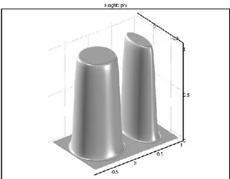
Figure. 1.1 Schematic of microscale (Kn <<1) and nanoscale (Kn >1) chambers.

Hydrodynamic Characteristic Times - In micro-hydrodynamics,

four characteristic times are usually defined. These times will be used in the following sections to establish some dimensionless groups:

a) The convective (or viscous) time scales the time for a

perturbation to propagate in the liquid

𝜏_𝐶 = 𝑅/𝑉 (1.18) where R is a dimension and V is the velocity of the liquid. Depending on the flow configuration (shear or elongational), the convective time may also be written as

𝜏_𝐶 = 1

𝛾 or 1

𝜀 (1.19)

13 b) The diffusional time is the time taken by a perturbation to diffuse in the liquid

𝜏_𝐷 = 𝑅2

𝜐 (1.20)

where, 𝜐 = m/ρ is the kinematic viscosity (units m2/s).

c) The Rayleigh time is a time scale of the perturbation of an

interface under the action of inertia and surface tension [3–5]

𝜏_𝑅 = 𝜌𝑅3

𝛾 (1.21)

Newtonian Fluids - The terms of Newtonian fluid (named after

Isaac Newton) is defined to be a fluid whose shear stress is linearly proportional to the velocity gradient in the direction perpendicular to the plane of shear [1] [2]. This definition means regardless of the forces acting on a fluid, it continues to flow. For example, water is a Newtonian fluid, because it continues to display fluid properties no matter how much it is stirred or mixed. A slightly less rigorous definition is that the drag of a small object being moved slowly through the fluid is proportional to the force applied to the object. (Compare friction). Important fluids, like water as well as most gases behave to good approximation as a Newtonian fluid under normal conditions on Earth

Let us mention here that usual liquids like water belong to the Newtonian category and polymeric fluids belong to the non-Newtonian category. The Reynolds number characterizes the

14

relative importance of inertial and viscous forces. It is usually written under the form

Re = V R / ν (1.22)

where, V is the average fluid velocity and R is a length characteristic of the geometry.

𝑅𝑒 = 𝜌𝑉2

𝜇 𝑉/𝑅 (1.23)

The Reynolds number is the ratio of a dynamic pressure-linked to inertia-to shearing stress-pressure-linked to viscous forces. In microfluidics, the Reynolds number is generally small, corresponding to a laminar flow regime [1] [2]. Very few microfluidic systems use turbulent flows. It is recalled here that, in enclosures, a number of Reynolds of 2,000 is required to reach the transition to turbulence. A more subtle sub classification can be made for the laminar regime. A very low Reynolds number (less than 0.5) indicates a creeping flow, for which the Stokes approximation is valid, this is the general case.

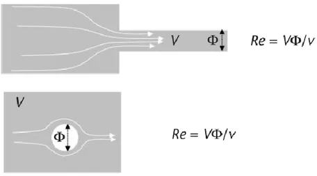
However recently, with the development of micro systems for cells handling, larger velocities are often used corresponding to Reynolds numbers in the range from 1-20. Figure 1.2 schematizes the definition of the Reynolds number for some geometrical configurations.

15

Figure 1.2 Reynolds numbers: (a) Reynolds number in a channel and (b) Reynolds number around a spherical particle.

Capillary Number- It is very important in two-phase microfluidics.

It compares viscous/elongational forces to surface tension forces. The capillary number can take different forms, depending on the physics of the problem. It can be built using the average velocity,

the shear rate, or the elongational rate:

𝐶𝑎 = 𝜂𝑉 𝛾 (1.24)

𝐶𝑎 = 𝜂𝛾 𝑅 𝛾 𝐶𝑎 = 𝜂𝜖 𝑅 𝛾

Remarking that the shear stress can be written ηVR, η𝛾 , η 𝜀 depending on the specific configuration, and the capillary pressure

γ/R, one immediately sees that the capillary number is the ratio of

the viscous forces to the capillary forces [1] [2].

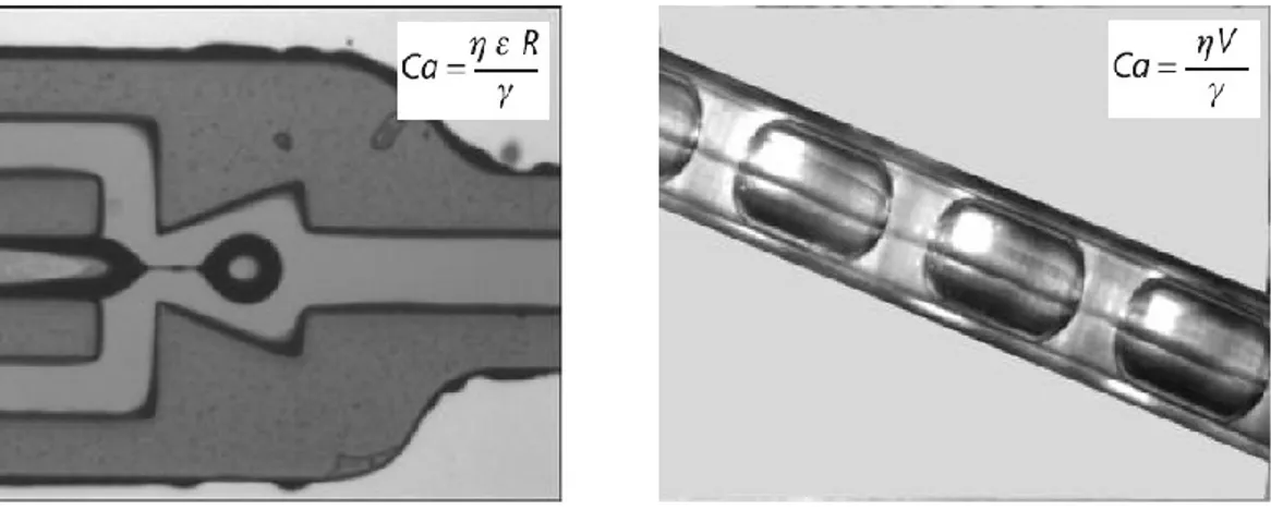
Let us illustrate this remark by two examples. In flow focusing devices (FFD), the capillary number is a relevant criterion to predict liquid thread breakup see figure 1.3(a). In this case, the capillary number is built on the shear rate (or elongation rate).

16

As the filament stretches and thins down, the capillary number decreases and when it becomes less than a critical value

Cacrit ~ 0.1 to 0.01, the surface tension forces break the liquid

filament into droplets, minimizing the interfacial area (hence the surface energy); this phenomenon is usually called the Rayleigh-Plateau instability.

In a plug flow, the friction of the plugs with the walls is a function of the capillary number of the liquid of the plugs shown in figure 1.3(b).

Figure 1.3 (a) Capillary number for an elongating liquid thread in a flow focusing device (FFD) and (b) capillary number for plug flow in a tube.

Weber Number

The Weber number is used to predict the disruption of an interface under the action of strong inertial forces [1]. More specifically, the Weber number is the ratio of inertial forces to surface tension forces

𝑊𝑒 = 𝜌𝑉2𝑅 𝛾 = 𝜌𝑉2 𝛾 𝑅 (1.25)

17

The numerator corresponds to a dynamic pressure ρV2 and the denominator to a capillary pressure γ/R. A strong surface tension maintains the droplet as a unique microfluidic entity with a convex interface. If the inertia forces are progressively increased, the interface is first deformed by waves, becomes locally concave, and is finally disrupted.

Ohnesorge Number- It relates the viscous and surface tension

forces. It is defined as

𝑂𝑕 = 𝜂

𝜌𝛾𝐿 =

𝑊𝑒

𝑅𝑒 (1.26)

The Ohnesorge number has been shown to be a good criterion to predict the breakup of liquid jets in a gas. Another expression seldom used for the comparison of viscous and surface tension forces is the Laplace number defined by

𝐿𝑎 = 1 _𝑂𝑕2 (1.27)

Dean Number - It is a dimensionless group in fluid mechanics,

which occurs in the study of flow in curved pipes and channels [1]. The Dean number is typically denoted by the symbol De for flow in a pipe or tube. it is defined as:

𝐷𝑒 = 𝜌𝑉𝐷 𝜇 𝐷 2𝑅 1/2 (1.28)

where ρ is the density of the fluid, μ is the dynamic viscosity, V is the axial velocity scale, D is the diameter (other shapes are represented by an equivalent diameter, see Reynolds number), and

R is the radius of curvature of the path of the channel. The Dean

18

axial flow V through a pipe of diameter D) and the square root of the curvature ratio.

Péclet Number – It is a dimensionless number relevant in the study

of transport phenomena in fluid flows. It is named after the French physicist Jean Claude Eugène Péclet [1] [2]. It is defined to be the ratio of the rate of advection of a physical quantity by the flow to the rate of diffusion of the same quantity driven by an appropriate gradient.

In the context of the transport of heat, the Péclet number is equivalent to the product of the Reynolds number and the Prandtl number. In the context of species or mass dispersion, the Péclet number is the product of the Reynolds number and the Schmidt number.

𝑃𝑒 = 𝑢∙𝑊

𝑑 (1.29)

In engineering applications, the Péclet number is often very large. In such situations, the dependency of the flow upon downstream locations is diminished, and variables in the flow tend to become 'one-way' properties. Thus, when modeling certain situations with high Péclet numbers, simpler computational models can be adopted.

1.2 Two Phase Microfluidics

The two-phase flows are characterized by the presence of two phases of the same component and they represent the simplest case of multiphase flows. To be precise it should also use the term

19

multi component to indicate the flows consist of elements belonging to chemically different phases.

For example, a flow of water and steam is mono-phase component, while a stream of water and air is bi-phase component. The two-phase flows play a crucial role in the systems lab-on-a-chip. They are obtained by sliding simultaneously two different fluids within a single micro channel. May be composed of two immiscible liquids, such as oil and water, or by a liquid phase and a gaseous [2] [3]. Microfluidic applications In two-phase, very often, is useful carry two different fluids in order to prepare them for subsequent analysis, get any reaction or perform chemical analyzes.

The analytical solutions to the Navier–Stokes equation are: the pressure-driven, steady state flows in channels, also known as Poiseuille flows or Hagen–Poiseuille flows. This is major importance for the basic understanding of liquid handling in lab-on-a-chip systems [1] [2] [3].

Poiseuille flow - In a Poiseuille flow, the fluid is driven through a

long, straight, and rigid channel by imposing a pressure difference between the two ends of the channel [1]. Originally, Hagen and Poiseuille studied channels with circular cross-sections; as such channels are straightforward to produce. However, especially in microfluidics, one frequently encounters other shapes.

Hydraulic resistance - In section 1.2, the Poiseuille flow has

explained for the pressure-driven, steady-state flow of an incompressible Newtonian fluid through a straight channel that a constant pressure drop Δp resulted in a constant flow rate Q. This result can be summarized in the Hagen-Poiseuille law.

20

𝛥𝑝 = 𝑅_𝑕𝑦𝑑𝑄 = 1

𝐺𝑕 𝑦𝑑 𝑄 (1.30)

The hydraulic resistance can be defined as the property that presents a pipeline to oppose the flow of a fluid inside of it. It may be constant or variable according to the specific operating conditions of the system. In Fluid dynamics, the concept of hydraulic resistance is related to the law of Poiseuille (or also of Hagen-Poiseuille) [1]. It shows that in a conduit where a viscous fluid flows in laminar regime, to parity of the other parameters, the flow rate is proportional to the pressure difference applied across the duct.

The Hagen–Poiseuille law, equation 1.30, is completely analogous to Ohm’s law, Δ𝑉 = 𝑅𝐼 relating the electrical current I through a wire with the electrical resistance R of the wire and the electrical potential drop ΔV along the wire. The SI units used in the Hagen–Poiseuille law are:

𝑄 = 𝑚 3 𝑠 , Δ𝑝 = 𝑃𝑎 = 𝑁 𝑚2 = 𝑘𝑔 𝑚𝑠2, 𝑅𝑕𝑦𝑑 = 𝑃𝑎𝑠 𝑚3 = 𝑘𝑔 𝑚4_𝑠

The concept of hydraulic resistance is fundamental to the characterization of micro-channels of a microfluidic system. The hydraulic resistance depends strongly on the section of the duct: increases as the length of the pipe L and decreases with the tube section.

Also increases proportionally with respect to the viscosity of the fluid. Below are expressions for the calculation of the hydraulic resistance in the case of some specific conducted to vary the section:

21

Table. 1.1. Hydraulic resistance for straight channels with different cross-sectional shapes.

where L indicates the length of the channel (not is a sectional dimension), while η is the dynamic viscosity of the fluid. When two channels are connected to form a channel longer, not always the law of Poiseuille turns out to be still valid. Check that the Reynolds number is sufficiently low:

Section of the channel Hydraulic Resistance

Circle (radius a) a 8

πηL 1 a4

Elliptical a

(major axis a, minor axis b) b

4 πηL 1 + (b/a)2 (𝑏/𝑎)2 1 a4

equilateral triangular (side a) a 320

3 ηL 1 a4 parallel walls h ( height h, width w) w 12ηL 1 wh3 Rectangular h ( altezza h, larghezza w) w 12ηL 1 − 0.63(_wh) 1 wh3 Square (side a) a 12ηL 1 − 0.917 ∗ 0.63 1 h4

22

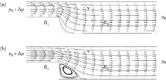
Fig. 1.4. (a) Two channels in series with down Re; (b) Two channels in series with Re too high.

In figure 1.4 shows a case in which the Reynolds number (Re) is sufficiently small: we can assume still valid as the law of

Poiseuille and write ∆𝑃 = 𝑅₁ + 𝑅₂ 𝑄 in the case of figure 1.4(b)

instead Re is such as to have the formation of a "convective motion", Poiseuille's law is not applicable.

Assuming a value of 𝑅𝑒 ≥ 0 is therefore possible to consider the series of two resistors hydraulic and write so that the equivalent resistance is:

R = R1+R2 (1.31)

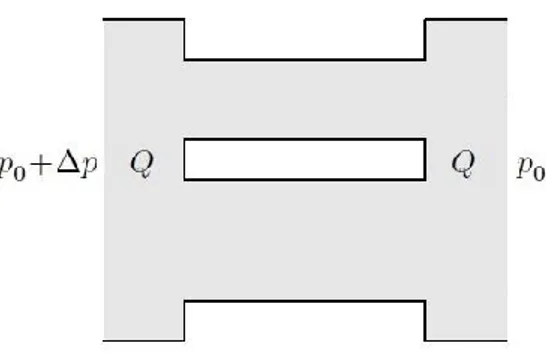
It is also possible to consider two channels connected in parallel as in figure 1.5. Assuming the same conditions with respect to the Reynolds number will have the following equivalent resistance:

𝑅 = 1

𝑅1+

1

23

Fig. 1.5. Two channels connected in parallel

Hydraulic Capacity - In the previous paragraph has been discussed

the analogy between the Poiseuille's law and Ohm's law: it evidently known as the change in pressure ΔP and the flow rate Q (volume V of unit of time) correspond respectively to the potential difference ΔU and the current (charge q of units of time) [1].

Similarly to the case of resistance, starting from the definition of electric capacity

𝐶 = 𝑑𝑞

𝑑𝑈 (1.33)

that the concept of hydraulic capacity given by the following expression:

𝐶_𝑕𝑦𝑑 = −𝑑𝑉

𝑑𝑃 (1.34)

where the minus sign indicates a reduction of the volume as the pressure increases.

The hydraulic capacity exists because neither the real fluids nor the channels containing them are totally rigid, but have certain elasticity. Their volume changes, often even of a small amount, varying the environmental pressure. This implies the property of an element such as a channel or a tank to store a greater or lesser

24

amount of fluid, which results in a determined value of hydraulic capacity. Generally it can be considered constant and the hydraulic capacity given by the following expression:

𝐶 = ∆𝑉

∆𝑝 (1.35)

In the SI is measured in m3/Pa. Until now in microfluidic

technology, it was possible to realize elements of hydraulic capacity variable by making use of elastic materials that change their shape depending on the amount of liquid they receive.

1.3 Computational Fluidic Dynamics (CFD).

Theory and modeling methods can be conveniently classified into four groups, depending on the length and times scales to which they imply

a) The electronic scale of description in which matter is

regarded as made up of fundamental particles (electron, protons, etc.) and is described by quantum mechanics;

b) The atomistic level of description, in which matter is made

up of atoms, whose behavior obeys the laws of statistical mechanics;

c) The mesoscale level, in which matter is regarded as

composed of blobs of matter, each containing a number of atoms; and

d) The continuum level, in which matter is regarded as a

continuum, and the well-known macroscopic laws (equations of continuity and momentum conservation, constitutive equations such as Fourier’s law, etc.) apply.

25

For most fluids, the scale of tens or hundreds of micrometers is well suited to the standard continuum description of transport processes, even though surface forces play a more important role than in macroscopic applications. Continuum methods for computations of two fluids flows are based on macroscopic conservation laws for mass, momentum, and energy [1] [2]. They rely on the coupling of a method for description of the phase evolution often expresses the conservation of phase with a solver for the momentum equation and the energy equation. Here, the full non-linear problem and do, therefore, not consider methods that are limited to Stokes flow, such as the boundary integral method.

In the following, first various methods for description of the interface evolution and then consider the coupling of these algorithms with equation describing the transport of momentum, species mass and energy. Detailed information about these balance equations can be found in various text books.

There are two main numerical methods for simulating multiphase flow in microfluidics: interface tracking methods and interface capturing methods. The latter class of methods is ideal for simulation of immiscible two-fluid systems.

Interface Tracking Methods – In interface tracking methods (or

sharp-interface methods) the computational mesh elements lies in part or fully on fluid-fluid interfaces. Such methods, including boundary-integral methods, finite element methods, and immersed boundary methods, are a very accurate instrument for simulating the onset of breakup and coalescence transitions but encounter difficulties in simulating through and the past transitions [3].

26

Interface Capturing Methods – Simulations through breakup and

coalescence transitions using interface capturing methods (lattice – Boltzmann and lattice gas, constrained –interpolation-profile, level set, and volume of –fluid, couple level set, partial miscibility-model and phase field methods) do not require mesh cut and connect operations because the mesh elements do not lie on the interface, but rather the interface evolves through the mesh.

The fluid discontinuities (e.g. density, viscosity) are smoothed and the surface tension force is distributed over a thin layer near the interface to become a volume force (surface tension being the limit as the layer approaches zero thickness). Interface capturing methods are then ideal for simulating breakup and coalescence in immiscible two-fluid systems (and the effect of surfactants) and for three or more liquid components, being especially powerful for microchannel design.

1.3.1 Level set.

Flow problems with moving interfaces or boundaries occur in a number of different applications, such as fluid-structure interaction, multiphase flows, and flexible membranes moving in a liquid. One possible way to track moving interfaces is to use a level set method. A certain contour line of the globally defined function, the level set function, then represents the interface between phases. With the Level Set application mode you can move the interface within any velocity field [2].

The level set method is a technique to represent moving interfaces or boundaries using a fixed mesh. It is useful for problems where the computational domain can be divided into two domains separated by an interface. Each of the two domains can

27

consist of several parts. Figure 8-13 shows an example where one of the domains consists of two separated parts. The interface is represented by a certain level set or iso-contour of a globally defined function, the level set function. In COMSOL Multiphysics, is a smooth step function that equals zero in a domain and one in the other, across the interface, there is a smooth transition from zero to one. The interface is defined by the φ 0.5 iso-contours, or the level set, of. Figure 8-14 shows the level set representation of the interface in figure 1.6.

Fig.1.6. Example of two domain divided by an interface. In this case, one of the domains consists of two parts. Figure 8-14 shows the corresponding level set representation

28

Fig. 1.7. Surface plot of the level set function corresponding to Figure 1.

Numerical methods for interfaces of zero thickness can be divided into two main groups depending on the type of the grid. In the first group, moving unstructured grids are used and the interface is treated as a boundary.

The interface is represented by a set of cell edges; this allows a precise representation of interfacial jumps in the physical variables on the zero thickness interfaces without any smoothing. Such methods are often based on the arbitrary Largranian-Eulerian formulation, where the interface is resolved by a moving mesh [2]. Local mesh adaptations including mesh coarsening and mesh refining can be performed for both the interior and the interface elements to maintain good mesh quality, to achieve enough mesh resolution, to capture the changing curvature, and to obtain computational efficiency. However handling topological transitions of fluids particles such as coalescence, breakup and pinch-off requires rather complex algorithms.

In this review, the focus is on the second group of methods. In these the momentum equation is solved on a structured grid and an interface representation and advection algorithm is required to

29

define its motion across the computational domain. These methods may be divided into two classes. In front-capturing methods, the interface is implicitly embedded in a scalar field function defined on a fixed Eulerian mesh, such as a Cartesian grid. The second category is given by Lagrangian front-tracking methods, in which the interface is explicitly represented by Lagrangian particles and its dynamics is tracked by the motion of these particles. Among the front-capturing methods are the volume-of-fluid (VOF) and level set (LS) method which are, at least in their simplest version, relatively simple to implement. An early Lagrangian method is Marker in Cell (MAC) method where a fixed number of discrete Lagrangian particles are advected by the local flow.

The distribution of these particles identifies the regions occupied by a certain fluid. Lagrangian techniques emerged with the front-tracking (FT) method which uses surface markers. FT methods can give a more precise evolution of a deforming interface, but they may be relatively complex, with their need to book-keep logical connections among surface elements [2] [3]. In the following, discussion of the level set methods in a brief.

The level set method was introduced by osher and sethian as a general technique to capture a moving interface. It has subsequently been applied to two phase flows as well as in many other fields. The basic idea of the level set method is to represent the interface by the zero level set of a smooth scalar function

𝜙 𝑥 : 𝑅𝐷 → 𝑅, Γ = 𝑥: 𝜙 𝑥 = 0 .

Thus, the position of the interface is only known implicitly through the nodal values of 𝜙. In order to extract the position of the interface, an interpolation of the 𝜙 data on the grid points must be performed. One often mentioned advantage of the level set method

30

is its ability to handle topological changes and complex interfacial shapes in a simplified way. In practice, the level set function 𝜙 is initialized as the signed distance from the interface. For description of the interface evolution the phase indicator function in

𝐷𝑋±

𝐷𝑡 =

𝜕𝑋±

𝜕𝑡 + 𝑢 ∙ ∇𝑋± = 0; is replaced by 𝜙.

This level set equation is solved with high-order numerical discretization schemes in time and space, e.g. third-order total variation diminishing (TVD) Runge-Kutta schemes and third or fifth order Hamilton-Jacobi (HJ) weighted essentially non-oscillatory (WENO) schemes. Under evolution in time 𝜙 does not retain the property of a signed distance function and may develop steep and very small gradients. This results not only in inaccurate calculation of the interface normal vector and curvature but also in severe errors regarding mass conservation. For improved mass conservation of level set methods it is essential that 𝜙 stays a smooth function throughout the entire simulation. In order to achieve this, a reinitialization step is introduced, where the level set function is transformed into a scalar field that satisfies the properties of a signed distance function and has the same zero level set.

This reinitialization of 𝜙 is done in regular time intervals, often after each time step, but less frequent reinitializations are also common. For this reinitialization essentially two different methods are used in literature. Fast marching methods solve the Eikonal equation 𝛻𝜙 = 1 by computing the signed distance value for points in the computational domain or in a narrow band near the

31

interface. A more efficient and popular approach is to use a partial differential equation to reinitialize the level set function. Sussman et al. proposed to solve the following transient problem to steady state.

𝜕𝜙

𝜕𝜏 = 𝑠𝑔𝑛 𝜙0 (1 − 𝛻𝜙 )

𝜙 𝑥, 𝜏 = 0 = 𝜙₀(𝑥) (1.36)

Here, 𝜏 is the virtual time for reinitialization, 𝜙₀ is the level set function at any computational instant, and sgn(x) is a smoothed signum function which Sussman et al. approximated numerically as

𝑠𝑔𝑛 𝜙₀ = 𝜙0

𝜙₀2+ 𝐿2𝜖

(1.37)

Here, 𝐿_𝜀 is a small length scale to avoid dividing by zero, usually chosen as the mesh size. Equation 1.37 has the formal property that 𝜙 remains unchanged at the interface and converges to 𝛻𝜙 = 1 away from the interface. Russo and Smereka showed that the discretized version of equation 1.37 can displace the zero level set and may lead to substantial errors due to the reinitialization; as a remedy they proposed a fix for the redistance step discretization of Sussman et al [2]. recently, Hartman et al. presented two new improved formulations of the methods of Sussman et al. and Russo and Smereka for differential equation-based constrained reinitialization of the level set method.

Different temporal discretization schemes for solution of equation 1.37 were investigated by min. However, even with a frequent reinitialization step the level step method tends in long time simulations to shrink convex iso-surfaces, i.e. it leads to mass

32

loss. To correct this mass loss, global as well as local mass correction steps have been proposed to explicitly enforce mass conservation.

1.3.2 Phase field.

The phase field method offers an attractive alternative to more established methods for solving multiphase flow problems. Instead of directly tracking the interface between two fluids, the interfacial layer is governed by a phase field variable. The surface tension force is added to the Navier-Stokes equations as a body force by multiplying the chemical potential of the system by the gradient of the phase field variable [2].

The evolution of the phase field variable is governed by the

Cahn-Hilliard equation, which is a 4th-order PDE. The Phase

Field application mode decomposes the Cahn-Hilliard equation into two second-order PDEs. For the level set method, the interface is simply convected with the flow field [2] [3].

The Cahn-Hilliard equation, on the other hand, does not only convect the fluid interface, but it also ensures that the total energy of the system diminishes correctly. The phase field method thus includes more physics than the level set method. The free energy of a system of two immiscible fluids consists of mixing, bulk distortion, and anchoring energy. For simple two-phase flows, only the mixing energy is retained, which results in a rather simple expression for the free energy.

The phase field method which is a special kind of diffuse interface method it stems from physical modeling. In diffuse interface (DI) methods, the infinitely thin boundary of separation

33

between twp immiscible fluids in the sharp interface limit is replaced by a transition region of small but finite width, across which physical properties vary steeply but continuously. The DI treatment can be motivated physically/thermodynamically or numerically as a regularization of the sharp interface limit. Anderson et al. mention three main advantages of diffuse interface (DI) methods. First, from a computational point of view, modeling of fluid interfaces as having finite thickness greatly simplifies the handling of topological changes of the interface, which can merge or breakup while no extra coding is required.

Second, the composition field has physical meanings not only on the interface but also in the bulk phase. Therefore, this method can be applied to many physical states such as miscible, immiscible, and partially miscible ones. Third, the method is able to simulate contact line motion as the contact-line stress singularity in the immediate vicinity of the contact line is removed. The most significant advantage in the present context is, however, that explicit tracking of the interface is unnecessary and all governing equations can be solved over the entire computational domain without any a priori knowledge of the location of the interfaces [2]. Phase field (PF) models can be considered as a particular type of

DI models that are based on fluid free energy.

The basic idea is to introduce a conserved order parameter or phase-field 𝜙, to characterize the two different phases. This order parameter changes rapidly but smoothly in the thin interfacial region and is mostly uniform in the bulk phases, where it takes distinct values 𝜑₊ and 𝜑₋, respectively. The interfacial location is

34

dynamics is modeled by an evolution equation for 𝜑, the Cahn-Hilliard equation.

𝜕𝜑

𝜕𝑡 + 𝑢 ∙ 𝛻 𝜑 = 𝛻 ∙ 𝑀𝛻𝜇𝜑 (1.38)

Here, 𝑀 𝜑 is a diffusion parameter, called the mobility. The chemical potential, 𝜇_𝜑, is the rate of change of free energy with respect to 𝜑 and is given by

𝜇_𝜑 = 𝑑𝜓

𝑑𝜑 − 𝜀𝜑

2_𝛻2 _(1.39)

For the bulk energy density 𝜓 𝜑 different formulations are

used in the literatures which depend on the choice for 𝜑_± .

Commonly used forms are examples. 𝜓 = 𝜑2 _{1 − 𝜑}2 _{∕ 4 for 𝜑}

+ = 1, 𝜑−= 0 (1.40)

and 𝜓 = 𝜑 + 0.5 2 _{𝜑 − 0.5} 2 _for𝜑

± = ±0.5. (1.41)

With equation 1.39, Cahn-Hilliard equation 1.38 involves fourth-order derivates with respect to 𝜑.

This makes its numerical treatment more complex as compared to the Navier Stokes equation which involves only second order derivates. The parameter 𝜀_𝜑 in equation 1.39 is a capillary width indicates of the thickness of the diffuse interface.

The Cahn number 𝐶𝑛 ≡ 𝜀_𝜑 𝐿_𝑐 relates 𝜀_𝜑 to a characteristic

macroscopic length 𝐿_𝑐.

An important issue in the phase field method is the