CRITICAL EVALUATION OF AN INTERCALIBRATION PROJECT FOCUSED ON THE DEFINITION OF NEW MULTI-ELEMENT SOIL
REFERENCE MATERIALS (AMS-MO1 AND AMS-ML1) Livia Vittori Antisari (1), Gianluca Bianchini (2), Enrico Dinelli (3),
Gloria Falsone (1), Aldo Gardini (4), Andrea Simoni (1), Renzo Tassinari (2), Gilmo Vianello (1)
(1) Department of Agricultural Sciences, University of Bologna, Italy (2) Department of Physics and Earth Sciences, University of Ferrara, Italy
(3) Depart. of Biological, Geological Environmental Sciences, University of Bologna, Italy (4) Department of Statistical Sciences “Paolo Fortunati”, University of Bologna, Italy Abstract
Soils are complex matrices and their geochemical investigation necessarily needs reliable Certified Reference Materials (CRMs), i.e. standards, to support analytical precision and accuracy. In particular, the definition of soil multi-element CRMs is particularly complex and involves an inter-laboratory program that employs numerous analytical techniques. In this study, we present the results of the inter-calibration experiment focused on the certification of two new soil standards named AMS-ML1 and AMS-MO1. The two soils developed on sandstone and serpentinite parent materials, respectively. The experiment involved numerous laboratories and focused on the evaluation of soil physicochemical parameters and geochemical analyses of major and trace elements by X-ray fluorescence (XRF) and Inductive Coupled Plasma techniques (ICP-OES and ICP-MS). The data was statistically elaborated. Three levels of repeatability and accuracy in function of the different analytical methods and instrumentation equipment was observed. The statistical evaluation of the results obtained by ICP-OES on Aqua Regia extracts (i.e., Lilliefors test for normally, Grubbs test for outliers, Cochran test for outliers in variances and ANOVA) allowed to computed some certified values for the two proposed soil standards. This preliminary study will represent the first step of a more thorough intercalibration ring-test involving a higher number of laboratories, in order to propose the investigated matrices as CRMs.
Keywords: standard soils, macroelements, microlements, XRF, Aqua Regia, ICP-OES, ICP-MS
Introduction
The international standards that govern the laboratories procedures for analytical testing (ISO 17025, EN 45001) give great importance to reliability and accuracy of the analytical methods and to results of the measurements (ISO 5725). In Italy the approval of the Official Methods of chemical analysis of soils (Gazzetta Ufficiale della Repubblica Italiana, 1999) had encouraged for workshops on procedures standardization for the soils analyses through calibration of both analytical techniques and procedures, involving several instruments. The ISO 5725 defines
the accuracy as the sum of the deviation from the true value or reference (trueness) and the variance between the results of analysis independently obtained on the same sample under the same operating conditions (precision). The concept of precision is better quantified through the use of two different parameters, the repeatability and the reproducibility of the results of the analysis. The first parameter (i.e., repeatability) describes the minimum variability between the results obtained from the analysis of the same sample, under the same environmental conditions, as well as instrumental setup, calibration and analytical time and technical operator. The second parameter (i.e., reproducibility) concerns the highest variability due to changes of the factors as time, instrument, environment, calibration and operator (ISO 5725/1). The repeatability is a estimate related to each laboratory and the reproducibility refers to interlaboratory comparisons (Giandon et al., 2012).
Two different soil standard materials were thus investigated by Experimental Center for the analysis and the study of the soil (CSSAS) to assess the different steps of standards preparation and statistical validation of results. The two standards, called AMS-ML1 and AMS-MO1, were used as internal reference materials. The concentration of total (X-ray fluorescence analysis: XRF) and pseudo-total elements (Aqua Regia mineralization: AR) has been investigated. The pseudo-total elements concentration in Aqua Regia mineralization solution was determined using Inductive Coupled Plasma (ICP) interfaced with both optical detector spectrometry (-OES) and mass spectrometry (-MS).
The aim of this study was the evaluation of elements concentration of which measurement has a good reproducibility and low variability comparing the three different methods: XRF, AR-ICP-OES, AR-ICP-MS. Finally, a further cross-check was obtained analyzing the samples by ICP-MS after effective dissolution obtained by repeated acid digestion by both fluoridric and nitric acids (HF-HNO3).
Materials
Soil sampling location
The sites chosen for the collection of the reference materials are located in the Upper Tuscan-Emilian Apennines on the border between the provinces of Bologna and Florence (Fig. 1). The first soil sample hereinafter referred to the abbreviation AMS-ML1, has been collected in Tuscany, in the town of Firenzuola, and is developed on a serpentinitic rock included in an allochthonous Liguride ophiolite unit. The second soil sample, called AMS-MO1, has been collected in Emilia Romagna, in the municipality of Monghidoro, and is developed on a sandstone rock included in the sedimentary flysch of Monghidoro formation. Both sites were characterized from the pedogenic point of view by opening control profiles, by description of the diagnostic horizons and their physical-chemical characterization by means of field and laboratory evaluations.
Figure 1
Location of the sampling sites (dashed circles in yellow):
AMS-ML1 site - Sasso Maltesca location (726 m
asl) Firenzuola hall, Tuscany Region.
Coord, Geogr.reference point WGS84 UTM 32T
691788.90 mE - 4899113.10 mN
AMS-MO1 site - Ardigò location (818 m asl)
Monghidoro hall, Emilia-Romagna Region. Coord, Geogr. reference point WGS84 UTM 32T 686903.42 mE - 4901041.04 mN
Parent material origin and characteristics
The AMS-ML1 soil parent material consists of serpentinite, an ultramafic rock of mantle provenance included in the Liguride Ophiolite association, i.e. remnants of oceanic lithosphere of Jurassic age obducted during the orogenic processes which originated the Apennines. This lithology is made of femic minerals such as olivine and pyroxenes which were mainly transformed in a serpentine-rich minerals suite.
Elements AMS-ML1 AMS-MO1 Table 1.
Average of major elements concentration performed by XRF on the pedogenetic substrates of AMS-ML1 (serpentinized peridotite rock) and AMS-MO1
(quartz-feldspathic sandstone rock) sites,
respectively M ac ro elem en ts ( o x id e % ) SiO2 37.03 69.03 TiO2 0.11 0.38 Al2O3 2.49 14.44 Fe2O3 10.22 2.98 MnO 0.19 0.10 MgO 35.70 1.42 CaO 0.29 0.81 Na2O 0.06 2.02 K2O 0.01 4.01 P2O5 0.01 0.03 LOI 13.89 4.78
The AMS-MO1 soil is slightly acidic and develops on sandstone, included in a flysch sedimentary sequence. The parent material was mainly composed by feldspars and quartz, with a carbonate-free matrix. The chemical compositions of both parent materials are reported in Table 1.
Participating laboratories
Preparation, homogenezation and storage of soil standard materials
- CSSAS, Experimental Centre for Soil Studies and Analysis, Alma Mater Studiorum, University of Bologna, Italy.
Physical-Chemical Analyses of soil standard materials
- CRAG, Research Centre for Soil-Plant System Studies, Agricultural Research Council, Gorizia, Italy.
- CRAR, Research Centre for Soil-Plant System Studies, Agricultural Research Council, Roma, Italy
- CRAS, Regional Agricultural Research Centre Regione Autonoma della Sardegna, Cagliari, Italy.
- CSA S.p.A., Rimini, Italy
- CSSAS, Experimental Centre for Soil Studies and Analysis, Alma Mater Studiorum, University of Bologna.
- DAES, Department of Agricultural and Environmental Sciences, University of Perugia.
- DIPSA, Department of Agricultural Sciences, Soil Chemistry and Pedology Area, University of Bologna, Italy.
- DISAT Laboratorio di Geopedologia e Pedologia Applicata, Dipartimento di Scienze dell’Ambiente e del Territorio, Università di Milano Bicocca, Italy.IAEC, Institute of Agricultural and Environmental Chemistry, Università Cattolica del Sacro Cuore, Piacenza, Italy.
Major and trace elements determination X ray fluorescence analyses (XRF)
- BIGEA, Department of Biological, Geological ant Environmental Sciences, University of Bologna, Italy
- DEPES, Department of Physics and Earth Sciences, University of Ferrara, Italy. ICP-OES and ICP-MS determination on Aqua regia solutions (called pseudo-total elements)
- CSSAS, Experimental Centre for Soil Studies and Analysis, Department of Agricultural Sciences, Alma Mater Studiorum, University of Bologna, Italy - DEPES, Department of Physics and Earth Sciences, University of Ferrara, Italy. - DIPSA, Department of Agricultural Sciences, Soil Chemistry and Pedology Area, University of Bologna
ICP-MS analyses on totally dissolved samples
Methods
Preparation, homogenization and storage of the material
Soil standard samples called AMS-MO1 and AMS-ML1 were obtained by homogenization of natural epipedon and endopedon layers collected down to a depth of 10 cm. Each standard sample was obtained by homogenization of about 300 kg of soil; soil samples were air-dried and sieved to 2 mm (fine earth fraction) the sample was subsequently subjected to quartering and division into portions of approximately 250 g.
Determination of physico-chemical characteristics
The main physico-chemical properties of soil reference material were determined according to the current Italian official methods for the physicochemical analysis of soils published on Gazzetta Uffciale (G.U. n 248/99). More in details, the fine earth (<2 mm) samples were analyzed for the following physical and chemical properties. Texture was measurd using wet sieving and sedimentation method (Day, 1965). Soil reaction (pH in H2O and in 1N KCl) was determined by a
potenziometer (1:2.5 soil:solution w/v) (pH-meter, Crison). Electrical conductivity (EC) was performed on the 1:2.5 ratio (w/v) using distilled water by a conductimeter (Orion). Total carbonate (CaCO3) content was quantified by
volumetric method (ISO 10693), according to Loeppert and Suarez (1996). Total organic C amount (TOC) was determined by wet oxidation with potassium dichromate at 160 °C for 10min according to Springer and Klee’s (1954) methodology. Total nitrogen content (TN) was measured by sulphuric acid digestion according to the Kjeldahl distillation method (Bremner and Mulvaney ,1982). Available phosphorus content (PCit) was extracted with a 1% citric acid solution and the P concentration was determined colorimetrically with the blue ammonium molybdate method with ascorbic acid as reducing agent according to
Watanabe and Olsen (1965).
Wavelength dispersive X-ray fluorescence analysis (WDXRF)
X-ray fluorescence (XRF) spectrometry enables the identification and quantification of an element by measurement of its characteristic X-ray emission wavelength of energy (Jenkins, 2006). XRF analysis is a well-established method of quantitative analysis of major (SiO2, TiO2, Al2O3, Fe2O3, MgO, MnO, CaO,
Na2O, K2O, P2O5, expressed in weigh percent) and trace elements (Ba, Ce, Co, Cr,
La, Nb, Ni, Pd, Rb, Sr, Th, V, Y, Zn, Cu, Ga, Nd and Sc expressed in parts per million) of any solid matrix. In laboratory, each standard sample was quartered again, dried at 60°C for 24 h in order to eliminate the hygroscopic water and then powdered using an agate mortar. Subsequently, an amount of about 4 g of powder were pressed with addition of boric acid by hydraulic press to obtain powder pellets. Simultaneously, 0.5-0.6 g of powder was heated for about 12 h in a furnace oven at 950°C in order to determine the loss on ignition (LOI). This parameter measures the concentration of volatile species contained in the sample.
XRF analyses were performed both at the University of Ferrara and at the University of Bologna.
- At Ferrara the analyses were carried out by a ARL Advant-XP spectrometer at the Department of Physics and Earth Sciences (DEPES). Calibrations were obtained analyzing certified reference materials, and matrix correction was performed according to ther method proposed by Traill and Lachance (1996). Precision and accuracy calculated by repeated analysis of numerous international standards (http://georem.mpch-mainz.gwdg.de/) having matrices comparable with those investigated, i.e. femic and ultrafemic rocks such as peridotites (JP-1, PCC-1, NIM-D, DTS-1), serpentinites (UBN), gabbros (JGb1, JGb2), felsic igneous rocks such as granitoids (AC-E, G-2, GA, GH, GS-N, GSR-1, GSP-1) and rhyolites (JR3, RGM1), and various typology of sedimentary rocks (JDO-1, JLK-1, JLS-1, JSD1, JSD2, JSD3). The errors were generally lower than 3% for Si, Ti, Fe, Ca and K, and 7% for Mg, Al, Mn and Na. For trace elements (above 10 ppm), the errors were generally lower than 10%.
- At Bologna the analyses were carried out by Philips PW 1480 spectrometer at the Department of Biological, Geological ant Environmental Sciences, (BIGEA), Alma Mater Studiorum University of Bologna, Italy. Major and trace element analyses were performed by X-ray fluorescence spectrometry on powder pellets, following the matrix correction methods of Franzini et al. (1972, 1975) and Leoni and Saitta (1976). The estimated precision and accuracy for trace element determinations are lower than 5% except for those elements concentration ≤10 ppm (10-15%). Total loss on ignition (LOI) was gravimetrically estimated after sample overnight heating at 950°C. CO2 was determined by gasvolumetry following the method of Fabbri et
al. (1973).
Aqua regia and HF+HNO3 soluble elements contents
The fine earth (<2mm) of soil standard samples were finely pulverized to <100 µm with an agate mill. An aliquot of approximately 250 mg of each homogenized and powdered sample was mineralized with Aqua Regia (6 mL 37% HCl Plus and 3mL 65% HNO3 Suprapur, E. Merck, Germany) in a microwave oven (Milestone 1200)
in a Teflon vessel using specific soil digestion program according to Ferronato et al. (2013) and Vittori et al. (2013). After cooling, solutions were made up to 20 mL with milli-Q water and then filtered with Whatman 42 filter.
Contents of 29 elements (Al, As, B, Ba, Be, Ca, Cd, Ce, Co, Cr, Cu, Fe, K, Li, Mg, Mn, Mo, Na, Ni, P, Pb, S, Sb, Sn, Sr, Ti, TI, V and Zn) were determined for both soil samples by:
- Inductive Coupled Plasma Optical Emission Spectrometry (ICP-OES, Spectro Ametek, Arcos and Spectro Ciros CCD) at the Experimental Centre for Soil Studies Analysis (CSSAS) and Department of Agricultural Sciences (DIPSA), Alma Mater Studiorum, University of Bologna, Italy. For the assessment of the instrumental method accuracy and the analytical results quality, the soil samples were prepared in duplicate and the International Reference Materials (BCR-CRM
141R, 142R, 143R, 320R) provided by the European Commission were used. These analyses will be hereafter referred as AR/ICP-OES.
- X Series Thermo-Scientific spectrometer at the Department of Physics and Earth Sciences of the University of Ferrara (DEPES). External calibration was obtained analyzing differently diluted standard solutions. Specific amounts of Rh, In and Re were added to the solutions as internal standard, in order to correct for instrument drift. Accuracy and precision, based on replicated analyses of samples and standards, are better than 10% for all elements, well above the detection limit. As reference standards, the E.P.A. Reference Standard SS-1 (B type naturally contaminated soil) and the E.P.A. Reference Standard SS-2 (C type naturally contaminated soil) were also analyzed to cross-check and validate results. These analyses will be hereafter defined as AR/ICP-MS. The above described ICP-MS analysis has been performed also on solutions obtained after acid digestion with HF+HNO3, a procedure that is more efficient than aqua regia in the dissolution of
silicate minerals. In this analytical protocol, 0.15 g were attacked for 12 hours with suprapure grade HF and HNO3 (6 and 3 ml, respectively) on Teflon beakers heated
at 170 °C on a hot plate. After evaporation, the samples are re-attacked with 3 ml of HF and 3 ml of HNO3, and then re-dried on the hot plate. The dried residua is
further re-dissolved with 4 ml of HNO3 and then evaporated. Finally, the residua is
solubilized with 2 ml of HNO3 and ultrapure water reaching a final volume of 100
ml. For these analyses the following reference standards have been used UBN (serpentinite), JGb-1 and JGb-2 (gabbros), JB-1 (basalt), GSR-2 (andesite), soils SS-1 and SS-2 (soils). These analyses will be hereafter defined as HF+HNO3
/ICP-MS.
Statistical approach
Statistical methods for aqua regia and ICP-OES determination. The dataset analysed consisted of a total of N=17 observations for each element divided into
K=4 groups, with the numerousness of the generic i-th group indicated by Ni.
An exploratory analysis of data was performed and for each group of each element the mean was computed as follow:
𝑋̅ =𝑖 ∑𝑁𝑖𝑗=1𝑥𝑖𝑗
𝑁𝑖 , 𝑖 = 1, … , 𝐾. [1]
And the corrected sample standard deviation:
𝑠𝑖 = √∑𝑁𝑖𝑗=1(𝑥𝑖𝑗−𝑋̅̅̅)𝑖2
𝑁𝑖−1 , 𝑖 = 1, … , 𝐾. [2]
Each set of data was subjected to a procedure of statistical analysis with the aim of identify the acceptable sets of results.
First of all, the null hypothesis that the data come from a normal distribution was tested by using the lillie.test, based on the Kolmogorov-Smirnov goodness of fit test. Verifying the normality assumption is essential since all the employed tests and elaborations assume the Normal distribution of the data. This family of tests is founded on the comparison between the empirical distribution and the specified theoretical distribution. In the case of the Lilliefors test, the latter is a Normal distribution function with parameter μ equal to the mean of the observations of each element 𝑋̅ and σ2 equal to the corrected sample variance s2. The test statistic D
is defined as:
𝐷 = max𝑋|𝐹∗(𝑋) − 𝑆
𝑁(𝑋)|, [3]
where 𝑆𝑁(𝑋) is the empirical distribution function and 𝐹∗(𝑋) is the normal
distribution function previously described. Then the obtained value is compared with the critical value D0.05 based on the Lilliefors distribution and the p-value is
computed by Monte Carlo methods (Lilliefors, 1967). If the resultant p-value is lower than the fixed confidence level of 0.05 then the null hypothesis tested is rejected. This procedure is implemented in R by the function lillie.test, included in the package nortest.
The second step consisted in testing for the homogeneity of the variances of the K data groups (with K=4). This is a crucial point since all the observations are analyzed with the same method, therefore homogeneous variances are expected. According to ISO Standard 5725 (1994), Cochran’s test for variance outliers was considered to investigate this. It assumes that the data groups come from a normal population and it is based on the C statistic which is defined as:
𝐶 =𝑙𝑎𝑟𝑔𝑒𝑠𝑡 𝑜𝑓 𝑡ℎ𝑒 𝑠𝑖2
∑𝐾𝑖=0𝑠𝑖2 [4]
.
Since in this case data had a balanced design and the only the upper limit variance was tested, the C statistic was compared with the critical value CUL with the
confidence level α=0.05: 𝐶𝑈𝐿 = [1 +𝐹 𝐾−1
𝑐(𝛼 𝐾⁄ ,(𝐾−1),(𝐾−1)(𝑁−1)]
−1
, [5]
where Fc is the critical value of a F distribution with K-1 and (K-1)(N-1) degrees of
freedom (Snedecor and Cochran, 1980). If C exceeds the threshold CUL, then the
null hypothesis that all the variances are homogeneous is rejected. This test was implemented in R by the function Cochran.test included in the package outliers. Afterward, the analysis focused on detecting outliers among the group means through the application of the Grubbs’ test for outliers. It is able to detect one outlier at a time and it can test the null hypothesis that no outliers are present in a vector assumed normally distributed. The G statistic is defined as:
𝐺 =𝑖 𝑖𝑛 1,..,𝐾max |𝑋̅̅̅−𝑌̅|𝑖
𝑠𝑌 , [6]
where 𝑋̅ is the mean of the i-th group, 𝑌̅ is the mean of the group means and 𝑠𝑖 𝑌 the standard deviation of the group means. For the one sided Grubbs’ test the null hypothesis is rejected when G is greater than the following critical value (Grubbs, 1950): 𝐾−1 √𝐾 √ 𝑡𝛼 𝐾,𝐾−2 2 𝐾−2+𝑡𝛼 𝐾,𝐾−2 2 , [7]
where 𝑡𝛼/2,𝐾−22 is the square of the value of the Student’s t distribution with K-2
degrees of freedom that corresponds to the α/2 quantile. The test was performed in R by using the function grubbs.test of the package outliers.
Ultimately, the estimate of the between group (Sb) and the within group (Sw)
standard deviations were compared by using the one way ANOVA. The two components of the overall variance are estimated by the following expressions: 𝑆𝑏 = √∑𝐾𝑖=1𝑁𝑖∙(𝑋̅̅̅−𝑌̅)𝑖 2
𝐾−1 , [8]
𝑆𝑤= √∑𝐾𝑖=1∑𝑁𝑖𝑗=1(𝑥𝑖𝑗−𝑋̅̅̅)𝑖 2
𝐾∙(𝑁−1) . [9]
The study of the variance decomposition estimated by the one way ANOVA showed that the between group variation represented the major source of variability, then it was decided to compute the certified value as the mean of the group means, indicated by 𝑌̅.
A 95% confidence interval was computed for every mean group, and its range was computed as:
𝑋̅ ± 𝑡𝑖 𝛼
2,𝑁𝑖−1∙
𝑠𝑖
√𝑁𝑖 [10]
The 95% confidence interval was also computed for the certified value in a similar way:
𝑌̅ ± 𝑡𝛼
2,𝑁−1∙
𝑠
√𝑁, [11]
where s in the estimated standard deviation of the group means: 𝑠 = √∑𝐾𝑖=1(𝑋̅̅̅−𝑌̅)𝑖 2
The uncertainty of the certified value was fixed as the half width of the 95% confidence interval of the mean 𝑌̅.
The tests on certifiable elements should not show any evidence of issues in the assumptions and the mean value has to be included in the confidence interval of every group mean. To verify this point, bar graphs for each element were produced. Results and discussion
Physicochemical properties of standard soils
The main physicochemical properties obtained by the different laboratories were shown in Tables 2 and 3. The textural class of both standard soils is sandy.
Table 2. Mean amount of textural classes (Sand, Silt and Clay) determined on AMS-ML1 e
AMS-MO1 standard materials, measured during 2010-2014 (Measure unit g/kg). * The da-ta is the mean value of 11 analytical replications.
Standard Laboratory number Sand 2-0.05 mm Silt 0.05-0.002 mm Clay < 0.002 mm Average (11)* SD Average (11)* SD Average (11)* SD AMS-ML1- 4 625 49 215 35 164 16 AMS-MO1 7 796 31 134 17 70 23
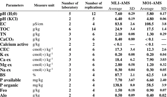
Table 3. Mean values of physicochemical properties of AMS-ML1 e AMS-MO1 soil
stand-ard materials, measured during 2010-2014.
Parameters Measure unit Number of
laboratory Number of replications ML1-AMS MO1-AMS Average SD Average SD pH (H20) 5 12 7.60 0.29 5.80 0.17 pH (KCl) 2 5 6.40 0.19 4.80 0.06 EC μS/cm 2 4 83.8 2.6 108.5 3.8 TOC g/kg 6 14 24.9 3.4 17.5 1.4 TN g/kg 3 6 2.10 0.08 1.30 0.29 CaCO3 g/kg 3 6 8.40 0.80 < 0.1 ----Calcium active g/kg 2 2 < 0.1 ---- < 0.1 ----CEC cmol(+) kg-1 4 6 17.3 3.4 12.3 2.6 K ex cmol(+) kg-1 3 6 0.20 0.08 0.20 0.04 Ca ex cmol(+) kg-1 3 6 18.4 6.2 7.90 3.03 Mg ex cmol(+) kg-1 3 6 2.80 0.58 1.20 0.32 Na ex cmol(+) kg-1 3 6 0.30 0.04 0.30 0.05 BS % 2 4 87.7 2.1 62.5 1.8 P available mg/kg 3 6 7.70 3.67 6.60 2.40 P organic mg/kg 2 4 138.8 8.0 58.5 3.9 Feo g/kg 2 4 1.50 0.18 0.90 0.07 Alo g/kg 2 4 0.50 0.09 0.40 0.02
Where: EC is Electric Conductivity; TN is total nitrogen ; TOC is Total Organic Carbon; CaCO3 is
total carbonate, CEC is Cation Exchange Capacity; K ex, Ca ex, Mg ex and Na ex are the exchangeable bases, BS is Base saturation, P available is P content according to Olsen’s method, Feo and Alo forms are Al and Fe extracted by ammonium oxalate solution
The two standard materials differ for some parameters as pH value which is neutral for ML1 and acid for MO1, the amount of exchangeable bases and percentage of basic saturation, which were lower in MO1 than in ML1-ASM, as expected due to the different parent material. Other properties are instead similar as high TOC and TN content in both soil standards (TOC: 24.9 and 17.5 g/kg, TN: 2.1 and 1.3 g/kg, respectively for AMS-ML1 and AMS-MO1). The cation exchange capacity (CEC) value is relatively high referred to the high sand content and it is due to high organic matter content. As expected, the prevailing phosphorus form for both standards is organic one, linked to high organic matter content.
Comparison of major and trace elements determination in soil standard materials using different analytical techniques.
The major and trace elements concentrations are detected using different methodologies. The Tables 4a,b and 5a,b showed the elements measured after mineralization using HF-HNO3 and HCl-HNO3 (aqua regia, AR) solution and
determined by ICP-MS.
As expected, the use of HF during the solubilization of samples makes the elements extraction more efficient than AR methodology. The ICP-MS instrument is a very powerful analytical tool due to a large amount of trace elements detected. Many of these are related to the group of rare-earth elements (REE) and these can be used as tracers of chemical-biochemical processes in soils. The sensibility of ICP-MS for determining the trace elements is very good according to the low standard deviation (SD).
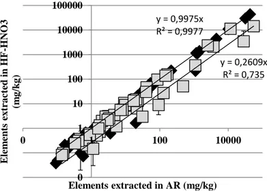
In Figure 2, the logarithmic scatterplot obtained from the comparison of HF-HNO3
data (Y axis) and Aqua Regia data (X axis) determined using ICP-MS tool of AMS-ML1 (black diamond) and AMS-MO1 (gray square) are shown.
Figure 2. Logarithmic scatterplot of the elements concentration determined in Aqua Regia (AR) vs HF-HNO3 solution using ICP-MS of MO1-ASM (gray square) and ML1-ASM (black diamond) y = 0,9975x R² = 0,9977 y = 0,2609x R² = 0,735 0 0 1 10 100 1000 10000 100000 0 1 100 10000 E lem ent s ex tra ct ed in H F -H NO 3 (m g /k g ) Elements extracted in AR (mg/kg)
It is possible notice that the results for ML1 are very similar for the two investigation (R2 = 0.998), while in AMS-MO1 lower value of determination
coefficient was found (R2 = 0.735) and lower amounts of K and Al were detected
using AR method than those obtained with HF-HNO3 mineralization.
Element
ICP-MS analyses on samples totally dissolved by HF+HNO3
Table 4a
Mean (2 samples) of major and trace elements concentration using
HF-HNO3 mineralization
coupled with ICP-MS tool for ML1 and AMS-MO1 samples
characterization. The data are expressed in mg/kg na not analysed, SD standard deviation. AMS-ML1 AMS-MO1 Average SD Average SD Al 31508 1279 55067 151 B 36.7 4.5 9.1 0.4 Ba 87.8 2.7 476 1 Be 0.68 0.10 1.7 0.2 Ca 10157 1780 3661 33 Cd 0.88 0.2 1.4 0.4 Co 75.6 0.2 3.1 0.1 Cr 1268 28.3 84.4 3.4 Cu 22.4 0.1 9.9 1.4 Fe 43163 4657 11564 215 Ga 9.00 0.8 21.3 7.6 K 4489 1195 28043 5547 Li 47.8 1.9 18.1 1.5 Mg na na 2515 245 Mn 1434 101 166 9 Mo 0.31 0.01 2.0 0.1 Na na na 14521 213 Ni 1153 44 9.70 0.80 P 214 10 147 2 Pb 8.88 0.10 22.6 2.2 Sb 0.24 0.01 0.50 0.01 Sc 9.08 0.10 2.60 0.40 Sn 1.28 0.30 3.30 0.10 Sr 62.1 0.6 92.0 5.3 Ti 1096 45 1088 11 Tl 0.17 0.01 0.70 0.01 Zn 53.3 0.7 41.1 6.3 Rb 28.0 0.4 128 7 Y 5.58 0.10 8.20 0.80 Zr 19.8 0.4 30.8 0.6 .
Element
ICP-MS analyses on samples totally dissolved by HF+HNO3
Table 4b
Mean (2 samples) of rare-earth elements (REE) concentration using
HF-HNO3 mineralization
coupled with ICP-MS tool for ML1 and AMS-MO1 samples
characterization. The data are expressed in mg/kg SD standard deviation AMS-ML1 AMS-MO1 Average SD Average SD Nb 3.58 0.10 5.40 0.20 La 9.05 0.10 20.5 3.0 Ce 18.2 0.30 39.7 5.6 Pr 2.15 0.01 4.60 0.50 Nd 8.19 0.20 17.2 1.7 Sm 1.59 0.01 3.30 0.30 Eu 0.36 0.01 0.70 0.01 Gd 1.52 0.01 3.00 0.30 Tb 0.23 0.01 0.40 0.01 Dy 1.06 0.01 1.80 0.10 Ho 0.22 0.01 0.30 0.01 Er 0.59 0.01 0.90 0.01 Tm 0.10 0.01 0.20 0.01 Yb 0.58 0.01 0.90 0.01 Lu 0.09 0.01 0.10 0.01 Hf 0.58 0.10 1.10 0.11 Ta 0.35 0.20 0.40 0.01 Th 2.27 0.10 7.20 0.01 U 0.48 0.10 1.60 0.20
The total dissolution of the soil samples using HF-HNO3 solution coupled with
ICP-MS tool showed similar concentration for many elements to those determined by X-ray fluorescence technique (XRF), as reported in Table 6. The results for major elements in XRF have been standardized using their percentage as oxides and the 100% of composition is given by the compounds loosen by ignition at 950°C (loss on ignition, LOI). The trace elements were expressed as mg/kg. The XRF method also allows to determine some elements of group of rare-earth (REE). The pseudo-total elements concentration is shown in Table 7. These elements are extracted from soil in Aqua Regia, and detected using ICP coupled with optical emission spectrometry (OES). It is well known that several elements could be overestimated or underestimated by ICP-OES due to the interference of some elements which can emit wavelengths of certain orbital levels in the same line. Nevertheless, the versatility of this instrument which determines simultaneously all the elements makes it very common in testing laboratories.
The comparison of the elements concentration in the AR-extracts determined by ICP-MS and ICP-OES (Table 4a and 7, respectively) showed several difference.
lement
ICP-MS analyses on samples dissolved by HCl+HNO3
Table 5a
Mean of major and trace elements concentration using aqua regia
mineralization coupled with ICP-MS tool for AMS-ML1 and AMS-MO1 samples characterization. The data are expressed in mg/kg na not analysed, SD standard deviation. AMS-ML1 AMS-MO1 Average (6) SD Average (6) SD Al 29583 1625 14423 613 As 3.60 0.29 4.10 0.48 B 41.7 2.8 10.8 1.0 Ba 87.1 2.5 51.3 2.0 Be 0.70 0.03 0.73 0.04 Ca 11070 476 2105 119 Cd 0.10 0.01 0.51 0.14 Co 77.5 2.8 3.10 0.10 Cr 1138 28 95.8 5.2 Cu 21.3 2.2 8.40 0.93 Fe 44219 2089 11332 1114 Ga 10.5 1.3 6.50 0.47 K 4406 236 3472 463 Li 59.4 2.7 14.2 0.7 Mg na na 2380 100 Mn 1391 76 158 5 Mo 0.38 0.08 1.99 0.06 Na 144 13 370 23 Ni 1160 137 8.90 0.96 P 224 5 139 2 Pb 9.30 0.52 13.0 0.4 Sb 0.24 0.05 0.37 0.05 Sc 10.3 0.7 2.98 0.26 Sn 1.15 0.15 2.37 0.16 Sr 56.1 1.9 8.85 0.10 Ti 218 25 364 42 Tl 0.20 0.02 0.20 0.03 Zn 69.2 10.2 46.8 6.5 Rb 28.2 2.8 27.5 2.6 Y 4.22 0.10 5.68 0.03 Zr 1.64 0.04 2.95 0.03 .
Element
ICP-MS analyses on samples dissolved by HCl+HNO3
Table 5b
Mean of rare-earth elements (REE) elements
concentration using aqua regia mineralization coupled with ICP-MS tool for ML1-AMS and MO1-ASM samples
characterization. The data are expressed in mg/kg SD standard deviation AMS-ML1 AMS-MO1 Average (6) SD Average (6) SD Nb 0.61 0.01 1.20 0.09 La 8.12 0.05 15.0 0.5 Ce 16.4 0.2 30.4 1.0 Pr 2.00 0.02 3.52 0.11 Nd 8.10 0.11 13.3 0.4 Sm 1.60 0.03 2.52 0.07 Eu 0.36 0.01 0.34 0.01 Gd 1.40 0.03 2.20 0.03 Tb 0.21 0.01 0.31 0.01 Dy 0.88 0.02 1.31 0.01 Ho 0.16 <0,01 0.24 0.01 Er 0.36 <0,01 0.62 0.01 Tm 0.05 <0,01 0.10 <0,01 Yb 0.25 0.01 0.54 0.01 Lu 0.04 <0,01 0.08 <0,01 Hf 0.07 <0,01 0.15 <0,01 Ta <0,01 <0,01 <0,01 <0,01 Th 1.57 0.01 5.60 0.10 U 0.10 <0,01 0.99 0.01 .
Larger differences were investigated for trace elements than major ones; for example an overestimated value was detected by ICP-OES for Sb and Zn due to interference with other emission lines (e.g. aluminum, iron).
The comparison between the data obtained from AR, HF-HNO3 mineralization,
XRF methodology and both ICP-MS and ICP-OES techniques for ASM-MO1 showed that concentration of aluminium was detected in this way: XRF>HF-HNO3-ICP-MS>>AR for both instrumental techniques. (Fig. 3). Thus the Al
content in soil samples in AR were underestimated, confirming the already observed trend for AR-ICP-MS and HF+HNO3-ICP-MS.
Other elements showed similar trend as K, Fe and Ca. In ASM-ML1 samples the AR-ICP-OES underestimated the Mg content compared to XRF technique. These elements are present in minerals and for this reason discrepancies among samples occurred due to both treatment and instrument techniques.
It is important to note that distinct analytical techniques, sometimes for particular elements, give different results and these differences are mainly related to the treatment of the sample.
Elements
XRF determination of standard materials Table 6
Mean concentration of total elements using XRF determination of standard materials ML1-AMS e MO1-AMS, respectively in BIGEA and DEPES laboratory in the three years 2012-2014. The data are expressed as mg/kg SD standard deviation. AMS-ML1 AMS-MO1 Average (8) SD Average (8) SD M a cr o element s o x y des (%) SiO2 39.10 2.00 70.33 0.70 TiO2 0.20 0.00 0.30 0.01 Al2O3 7.10 0.70 13.79 0.50 Fe2O3 6.10 0.40 2.02 0.20 MnO 0.10 0.01 0.05 0.01 MgO 27.40 2.00 1.09 0.20 CaO 1.70 0.10 0.73 0.10 Na2O 0.20 0.10 2.27 0.10 K2O 0.60 0.01 3.60 0.10 P2O5 0.10 0.01 0.09 0.01 LOI 17.30 1.40 5.73 0.20 M icro a nd t ra ce element s (mg /kg ) As 6 3 5 1 Ba 139 64 466 29 Ce 19 13 36 4 Co 95 10 3 2 Cr 1709 99 145 26 Cu 31 5 12 2 Ga 8 1 11 1 Hf 3 1 8 4 La 14 2 15 2 Nb 7 4 8 2 Nd 9 3 13 2 Ni 1653 133 12 2 Pb 13 4 28 3 Rb 35 4 144 13 Sc 10 6 7 3.4 Sr 76 11 100 14 Th 5 6 6 4 V 63 8 33 3 Y 6 2 16 3 Zn 63 5 29 6 Zr 35 8 116 16
Elements
AMS-ML1 AMS-MO1 Table 7
Mean Concentration of elements using qua regia-ICP-OES determination of standard materials ML1and AMS-MO1, respectively in CSSAS e DIPSA laboratory in the three years 2012-2014. (Data expressed as mg/kg) SD standard deviation. Average (17) SD Average (17) SD Al 25174 1848 13181 962.9 As 1.7 0.3 3.5 0.3 B 35.7 1.2 13.8 4.4 Ba 76.9 8.5 53.5 6.3 Be 0.5 0.0 0.7 0.0 Ca 10673 1000 2008 154 Cd 0.1 0.0 0.2 0.0 Ce 8.6 0.6 26.4 0.7 Co 70.4 3.6 3.4 1.5 Cr 1122 60 94.6 13.9 Cu 27.3 1.0 8.7 1.5 Fe 34640 1994 8796 513 K 4869 742 2653 511 Li 62.6 3.1 13.8 1.2 Mg 13983 8909 2331 109 Mn 1102 101 161 6.1 Mo 0.3 0.0 1.9 0.3 Na 387 80 504 152 Ni 1111 60 10.4 0.6 P 223 17.4 155 8.4 Pb 11.4 3.7 13.4 0.6 S 317 100 150 15 Sb 5.6 1.1 1.2 0.2 Sn 0.9 0.1 2.3 1.1 Sr 52.7 8.9 11.1 1.4 Ti 194 35 411 52 Tl 0.8 0.3 0.7 0.2 V 47.3 2.1 20.6 1.1 Zn 74.3 4.1 34.1 10.1
The XRF analyses carried out both at the Universities of Bologna and Ferrara are internally consistent. This technique directly analyses the sample powder without preliminary chemical treatments. It gives the “bulk” i.e. total concentration of the investigated matrices. It is therefore plausible that the XRF elements concentra-tions tend be higher than those observed by ICP analyses on Aqua Regia soluconcentra-tions that, although often referred as pseudo-total, do not dissolve the more resistant minerals. HF+HNO3 extractions are obviously more effective and generally
dis-solve the silicate minerals. However, also in this case the more resistant minerals (e.g. zircon, rutile, chromite, corundum) resist to the acid attack.
Moreover, HF+HNO3 extractions are sometimes affected by losses of volatile
elements having affinity with fluorine during the acid attack. However, specific differences in elements concentration due to the type of parent material of soil materials were evident. AMS-ML1 comes from serpentinite, a rock rich in serpentine minerals which are 1:1 trioctahedral minerals.
Figure 3
Scatterplot of different extraction methodologies
(Aqua regia, HF-HNO3)
and instrumental techniques (ICP-OES, ICP-MS, XRF) and in particular AR-ICP-OES (white circle), AR-ICP-MS (Black diamond),
HF-HNO3-ICP-MS (gray
square) and XRF (gray triangle) for ML1-ASM and MO1-ASM, respectively.
The data are expressed as mg/kg
Serpentines are unstable at pH<8 (Evans, 1992). In soils serpentines easily weather and lead to the formation of pedogenic chlorite, which is normally an unstable clay mineral (Schaetzl and Anderson, 2005). Efficient dissolution in acidic condition can occur in serpentine-derived soils, because of the weathera-bility of serpentine and its transformation products.
For this reason in AMS-ML1 the differences in elements concentration between mineralization procedures (AR and HF+HNO3) were minimized with respect to
those detected in AMS-MO1. This later developed on sandstone rich in feld-spars and mica, and elements such as Al, K, Fe and Ca compose resistant miner-als to AR digestion. Note that XRF technique is not affected by preliminary treatments which can introduce errors, but is less sensitive that the ICP tech-niques in revealing concentration at few ppm level.
On the contrary, ICP-techniques, that are more precise and accurate in the anal-ysis of trace elements, sometimes show problems in the investigation of major elements. The above considerations cannot be established a priori and have to be evaluated for each sample having specific composition.
0 20000 40000 60000 80000 0 20000 40000 60000 80000 0 50000 100000 150000 200000 0 50000 100000 150000 200000
Elements
Results of the statistical tests used to explore each set of results Lillefors test
for normality
Grubbs test for outliers
Cochran test for outliers in variances
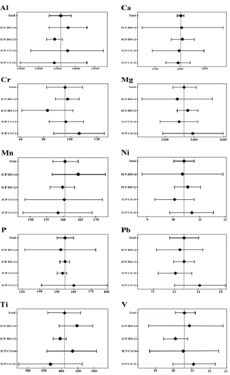
One way ANOVA D statistic p-value G statistic p-value C statistic p-value Sw Sb Al 0.152 0.376 0.916 0.444 0.585 0.139 853.018 986.592 Ca 0.182 0.143 1.145 0.776 0.548 0.206 168.747 47.994 Cr 0.158 0.308 1.340 0.426 0.335 1.000 22.127 11.177 Mg 0.154 0.354 1.327 0.755 0.444 0.512 110.318 99.803 Mn 0.158 0.314 1.649 0.129 0.544 0.214 6.193 5.463 Ni 0.117 0.779 1.485 0.410 0.559 0.183 0.633 0.567 P 0.199 0.073 1.449 0.135 0.526 0.255 8.607 7.243 Pb 0.103 0.905 1.621 0.170 0.372 0.862 0.554 0.913 Ti 0.111 0.838 1.382 0.628 0.506 0.307 47.423 71.146 V 0.102 0.909 1.288 0.565 0.472 0.411 1.085 0.920 Elements
Summary of the statistical data Table 8
Some examples of statistical tests on data obtained by aqua regia (AR) mineralization and ICP-OES determination of AMS-MO1 soil standard material. Mean of means SD of mean Certified value Uncertainty Al 13180.94 360.25 13180.9 573.2 Ca 2007.76 20.03 2007.8 31.9 Cr 94.59 8.97 94.6 14.3 Mg 2331.12 49.41 2331.1 78.6 Mn 160.73 2.35 160.8 3.8 Ni 10.42 0.24 10.4 0.4 P 155.00 3.13 155 5.0 Pb 13.45 0.40 13.5 0.7 Ti 410.61 30.60 410.6 48.7 V 20.65 0.37 20.6 0.6
.
ElementsResults of the statistical tests used to explore each set of results Lillefors test
for normality
Grubbs test for outliers
Cochran test for outliers in variances
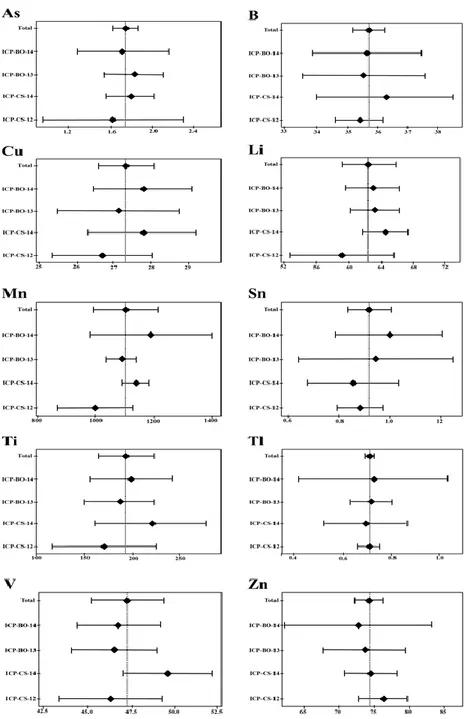
One way ANOVA D statistic p-value G statistic p-value C statistic p-value Sw Sb As 0.129 0.642 1.294 0.548 0.604 0.112 0.297 0.179 B 0.162 0.281 1.426 0.197 0.517 0.277 1.267 0.765 Cu 0.127 0.661 1.225 0.733 0.351 0.984 0.984 1.088 Li 0.148 0.414 1.442 0.156 0.562 0.178 2.634 4.660 Mn 0.145 0.445 1.294 0.549 0.653 0.062 79.849 164.923 Sn 0.112 0.823 1.212 0.768 0.467 0.426 0.146 0.130 Ti 0.157 0.319 1.258 0.645 0.478 0.389 33.535 42.261 Tl 0.119 0.755 1.229 0.724 0.619 0.095 0.298 0.061 V 0.116 0.784 1.490 0.027 0.343 1.000 1.740 3.131 Zn 0.099 0.929 1.332 0.447 0.622 0.091 4.257 3.051 Elements
Summary of the statistical data Table 9
Some examples of statistical tests on data obtained by aqua regia (AR) mineralization and ICP-OES determination of AMS-ML1 soil standard material Mean of means SD of mean Certified value Uncertainty As 1.747 0.08 1.7 0.2 B 35.711 0.33 35.7 0.6 Cu 27.350 0.47 27.4 0.8 Li 62.543 2.01 62.5 3.2 Mn 1102.562 71.31 1102.6 113.5 Sn 0.921 0.06 0.92 0.09 Ti 194.121 18.21 194.1 29.0 Tl 2.781 0.03 2.78 0.05 V 47.324 1.34 47.3 2.2 Zn 74.301 1.31 74.3 2.1
Figure 4. Some examples of statistical representation on data obtained by aqua regia (AR)
mineralization and ICP-OES of AMS-MO1 soil standard material (see also table 8). The data are expressed as mg/kg.
Figure 5. Some examples of statistical representation on data obtained by aqua regia (AR)
mineralization and ICP-OES of AMS-ML1 soil standard material (see also table 9). The data are expressed as mg/kg.
In general for most elements we noted that analyses on aqua regia solutions, analysed by both ICP-OES and ICP-MS, have lower concentration than analyses on solutions obtained treating the samples with HF+HNO3; in turn, the elements
concentration obtained on AR and HF+HNO3 solutions are usually lower than
sample powders by XRF.
Technical and statistical discussion
In Tables 8-9 and Figures 4-5 some examples of statistical tests on data obtained from AR-ICP-OES for AMS-MO1 and AMS-ML1 are shown. After statistical test we can certified some values obtained by AR-ICP-OES metodology (Tab. 8 and 9). Conclusions
The preparation of two reference materials (AMS-ML1 and AMS-MO1) obtained by homogenization of epipedon and endopedon of natural soils has allowed us to achieve a significant level of certification through ring tests carried out by some soil chemistry and geochemical laboratories in Italy. The statistical analysis of the data obtained has also highlighted the different levels of analytical sensitivity as a function of the methods and equipment used.
The comparison between the data obtained from Aqua Regia extracts and HF--HNO3-HCl mineralization determined by ICP-MS and ICP-OES, and from XRF
methodology showed several difference.
The XRF concentrations tend be higher than those observed with both ICP instruments analysing Aqua Regia solutions that, although often referred as pseudo-total, do not dissolve the more resistant minerals. HF+HNO3 extractions are
obviously more effective and generally dissolve the silicate minerals. Acknowledgments
Thanks to the scientific collaboration Anna Benedetti and Maria Teresa Dell’Abate
(Research Centre for Soil-Plant System Studies, Agricultural Research Council, Roma, Italy), Liviana Leita (Research Centre for Soil-Plant System Studies, Agricultural Research Council, Gorizia, Italy), Nicoletta Fadda (Regional Agricultural Research Centre Regione Autonoma della Sardegna, Cagliari, Italy), Elena Pari and Pierpaolo Tentoni (CSA S.p.A., Rimini, Italy), Rolando Calandra and Andrea Leccese (Department of Agricultural and Environmental Sciences, University of Perugia), Paola Gioacchini (Department of Agricultural Sciences, Soil Chemistry and Pedology Area, University of Bologna, Italy), Franco Previtali /(Laboratorio di Geopedologia e Pedologia Applicata, Dipartimento di Scienze dell’Ambiente e del Territorio, University of Milano Bicocca, Italy), Claudio Baffi e Sandro Silva (Institute of Agricultural and Environmental Chemistry, Università Cattolica del Sacro Cuore, Piacenza, Italy).
References
BREMNER J.M., MULVANEY C.S. (1982) Nitrogen-Total.” In: Methods of Soil Analysis. Agron. Madison. pp. 595- 624.
EVANS L.J. (1992) Alteration products at the earth’s surface – the clay minerals. In: Weathering, soils and paleosols. Elsevier, Amsterdam, London, New York, Tokyo
FABBRI B., GAZZI P., ZUFFA G.G. (1973) La determinazione della componente carbonatica nelle rocce. Mineral. Petrogr. Acta, 19:137-154.
FERRONATO C., VITTORI ANTISARI L., MODESTO M.M., VIANELLO G. (2013)
Speciation of heavy metals at water-sediment interface. EQA, 10:51-64. DOI 10.6092/ issn.2281-4485/3932.
FRANZINI M., LEONI L., SAITTA M. (1972) A simple method to evaluate the matrix effects in X-ray fluorescence analysis. X-ray Spectrometry, 1:151-154.
FRANZINI M., LEONI L., SAITTA M. (1975) Revisione di una metodologia analitica per fluorescenza X basata sulla correzione complete degli effetti di matrice. Rend. Soc. Ital. Mineral. Petrol., 31:365-378. A simple method to evaluate the matrix effects in X-ray fluorescence analysis. X-ray Spectrometry, 1:151-154.
GAZZETTA UFFICIALE DELLA REPUBBLICA ITALIANA (1999). Regolamento recante criteri, procedure e modalità per la messa in sicurezza e il ripristino ambientale dei siti inquinati, ai sensi dell’articolo 17 del decreto legislativo 5/2/1997, no 22, e successive modifiche e integrazioni 471:67.
GIANDON P., DALLA ROSA A., GARLATO A., RAGAZZI F. (2012) Evaluation of soil diffuse contamination in Venice region (Italy). EQA, 9:11-18. DOI 10.6092/issn.2281-4485/3733.
GRUBBS F.E. (1950) Sample criteria for testing outlying observations. Ann. Math. St., 21(1):27-58.
LOEPPERT, R.H., SUAREZ, D.L., (1996) Carbonate and gypsum. In: Sparks, D.L. (Ed.), Method of Soil Analysis. Part 3, Chemical Methods. SSSA and ASA, Madison, pp. 437– 474.
IMAI N., TERASHIMA S., ITOH S., ANDO A. (1996) Compilation of analytical data on nine GSJ geochemical reference samples. ‘’Sedimentary rock series’’. Geostand. Newsl., 20:165-216.
JENKINS R. (2006) Encyclopedia of Analytical Chemistry. Wiley. pp.21.
LEONI L., SAITTA M. (1976) X-ray fluorescence analysis of 29 trace elements in rock and mineral standards. Rend. Soc. Ital. Mineral. Petrol., 323:497-510.
LILLIEFORS H. (1967) On the Kolmogorov-Smirnov test for normality with mean and variance unknown. Journal of the American Statistical Association, 62:399-402.
SCHAETZL R., ANDERSON S. (2005) Basic concepts: soil mineralogy. In: Soils genesis and geomorphology. Cambrige University Press, Cambrige, UK. pp: 54-81
SNEDECOR G.W., COCHRAN W.G. (1980) Statistical methods. 7th ed. Ames: Iowa State
University Press.
SPRINGER U.. KLEE J. (1954) Prufung der Leistungfahigkeit vom Einigen Wichtigen Verfaren zur Bestimmung des Kohlensttoffe Mittels Chromschwefelsaure Sowie Vors- chlag Einer Neuen Schnellmethode.” Z. Pflanzenernahr. Dung. Bodenkunde. 1954. TRAILL R.J., LACHANCE G.R. (1966) Practical solution to the matrix problem in X-ray analysis. Canadian Journal of Spectroscopy, 11(2):43-48.
VITTORI ANTISARI L.. CARBONE S.. GATTI A.. VIANELLO G.. NANNIPIERI P. (2013) Toxicity of metal oxide (CeO2. Fe3O4. SnO2) engineered nanoparticles on soil
microbial biomass and their distribution in soil. Soil Biology and Biochemistry 60: 87-94. WATANABE F.S.. OLSEN S.R. (1965) Test of an ascorbic acid method for determining phosphorus in water and NaHCO3 extracts from soils. Soil Sci. Soc. Am. Proc.
UNE EVALUATION CRITIQUE DE PROIECT DE L’INTER ETALLONAGE AXES SUR DEFINITION DE NOUVEAUX MATERIAUX DE REFERENCE POUR L'ANALYSE CHIMIQUE DES SOLS (AMS-MO1 ET AMS-ML1)
Résumé
Les sols sont des matrices complexes et leur levé géochimique doit matériaux de référence certifiés (CRM) pour évaluer la précision de l'analyse et de précision. En particulier la préparation de matériaux de référence appropriés pour le contrôle des déterminations analytiques effectuées sur le sol nécessite un programme inter laboratoires avec l'utilisation de méthodologies et des instruments différentes. Dans cette étude, nous présentons les résultats de l'inter étalonnage axés sur la certification de deux nouvelles normes de sols appelés AMS-ML1 et AMS-MO1 origine respectivement sur les rochers de grès et de serpentine. L'activité expérimentale a impliqué de nombreux laboratoires et, en plus de l'évaluation des paramètres physiques et chimiques du sol, a mis l'accent sur le perfectionnement des techniques d'analyse par fluorescence X (XRF) et spectrométrie de masse (ICP-OES, ICP-MS ). L'analyse statistique a mis en évidence trois niveaux de répétabilité et la précision en fonction des différentes méthodes d'analyse et l'instrumentation utilisées. Dans le cas spécifique de l'extraction dans l'eau régale et de détermination dans les résultats d'ICP-OES, traitée en testant Lilliefors, Grubbs, Cochran et analyse de la variance, contribué à définir le niveau de certification pour certains éléments relatifs aux deux normes proposées. L'étude représente un premier niveau d'inter étalonnage et sera rendue plus épreuve de l'anneau avec l'aide de laboratoires plus spécialisés, de manière à obtenir la certification internationale.
Mots-clés: standard du sol, macro- micro éléments, XRF, Aqua Regia, ICP-OES, ICP-MS.
VALUTAZIONE CRITICA DI UN PROGETTO DI INTERCALIBRAZIONE MIRATO ALLA DEFINIZIONE DI NUOVI MATERIALI DI RIFERIMENTO PER ANALISI CHIMICHE DEI SUOLI (AMS-MO1 E AMS-ML1)
Riassunto
I suoli sono matrici complesse e la loro indagine geochimica ha bisogno di materiali certificati di riferimento (CRM) per valutarne la precisione analitica e l'accuratezza. In particolare la preparazione di materiali di riferimento idonei al controllo di determinazioni analitiche effettuate sul suolo richiede un programma interlaboratorio con l’impiego di metodologie e strumentazioni differenti. In questo studio vengono presentati i risultati dell'esperimento di intercalibrazione incentrato sulla certificazione di due nuovi standard di suoli denominati AMS-ML1 e AMS-MO1 originatisi rispettivamente su rocce arenacee e serpentinose. L'attività sperimentale ha coinvolto numerosi laboratori e, oltre alla valutazione di parametri chimico-fisici del suolo, si è concentrata sull’affinamento delle tecniche analitiche mediante fluorescenza a raggi X (XRF) e spettrometria di massa (ICP-OES, ICP-MS). L’elaborazione statistica ha permesso di evidenziare tre livelli di ripetibilità e precisione in funzione dei differenti metodi di analisi e della strumentazione utilizzata. Nel caso specifico dell’estrazione in Aqua Regia e determinazione in ICP-OES i risultati, elaborati mediante test di Lilliefors, di Grubbs, di Cochran e ANOVA, hanno permesso di definire il livello di certificazione per alcuni elementi riferiti ai due standard proposti. Lo studio rappresenta un primo livello di intercalibrazione e verranno effettuati ulteriori ring test con il contributo di più laboratori specializzati, in modo da conseguire una certificazione internazionale.