A macroeconomic model of bankruptcy

A MACROECONOMIC MODEL OF BANKRUPTCY

Roberto Tamborini

University of Trento, Department of Economics, Via Inama 5, 38100 Trento, Italy, Tel. 0461-882228, Fax. 0461-882222 E-mail: RTAMBORI@RISC1.GELSO.UNITN.IT

Workshop on Economics with Heteregenous Interacting Agents Ancona, May 30-31, 1997

FIRST DRAFT

Abstract

This paper relates to the macroeconomics of imperfect capital markets. In this framework, the heterogeneity of agents, notably of borrowing firms, is a key element in the explanation of interactions between financial intermediaries and borrowers facing a bankruptcy probability. This probability is usually introduced through exogenous stochastic factors in firms' revenue. In this paper I pursue a more inherently informational approach which, even though all market processes are deterministic, partly "endogenizes" the default probability as a consequence of heterogeneous, privately-held price expectations across firms. Then I examine in detail the credit transmission mechanism and its impact on the macroeconomic variables in an economy with characteristics such as those in 1) to 5).

J.E.L. Class.: E44, E51 (keywords: Macroeconomics, Imperfect capital markets, Credit and money)

_______________________

I wish to thank Piergiorgio Ardeni, Ottorino Chillemi, Domenico Delli Gatti, Marcello Messori, Michele Moretto and Gugliemo Weber for their helpful comments on earlier versions of this work. I remain fully responsible for this paper.

Introduction

This paper relates to the macroeconomics of imperfect capital markets, whose main features can be summarized as follows (e.g. Greenwald-Stiglitz, 1987, 1990; Gertler, 1988; Dimsdale, 1995; Ardeni et al., 1993; Tamborini, 1996):

1) Firms display heterogeneous unobservable characteristics, so that lenders may not be perfectly informed on firms' ability to pay. Consequently the various financial instruments whereby firms can raise means of payment are not perfect substitutes. Decisions about employment and production are conditional on the cost and contractual terms of the financial instruments available to firms.

2) "Credit is special", or "credit matters", in that it is the only source of means of payment for classes of firms which have no access to the open market. The particular nature of credit is that it forces the borrower and the lender to take account of the probability of bankruptcy.

3) Monetary policy matters to the extent that the central bank is able to alter "credit availability" to the economy (acting as regulator of, or as lender of last resort to, commercial banks).

In this framework for macroeconomic analysis, the heterogeneity of agents, notably of borrowing firms, is a key element in the explanation of interactions between lenders and borrowers. Relatedly, the causes and consequences of bankruptcy play a crucial role in explaining firms' behaviour and the whole macroeconomic process. These are major merits of the macroeconomics of imperfect capital markets. Whereas firms' fallibility is virtually ignored in standard macroeconomics, it is widely held among economists and businessmen that bankruptcy is the key social device whereby inefficient units are replaced by efficient ones in the competitive allocational process. There is also evidence, and a related large literature on corporate management, that businessmen do care about the eventuality of bankruptcy and the ensuing corporate as well as personal costs (see e.g. White, 1989; Altman, 1984).

Agents heterogeneity is closely connected with the study of bankruptcy. A trivial reason is that not all firms go bankrupt. To grasp heterogeneity, bankruptcy probability is usually introduced into the economy through exogenous stochastic factors specific to each firm's revenue whereby some firms default on their debt whereas others do not (see

e.g. Greenwald-Stiglitz, 1990, 1993). What makes this practice widely accepted is perhaps that it does not conflict with the principle that rational agents exploiting all available information correctly can only commit random errors. The advantage of considering bankruptcy under this assumption is recognition that a random error may be so large as to drive the agent out of the market. However, this analytical short-cut, though convenient, treats bankruptcy as pure misfortune and excludes any relation between bankruptcy and firms' behaviour or the macroeconomic process. By contrast, the business community and its ethics are built upon the principle of the entrepreneur's responsibility -though the unsuccessfull entrepreneur may be ready to blame his/her misfortune1.

In this paper I shall pursue a more inherently informational approach to bankruptcy based on heterogeneous, privately-held price expectations across firms. In other words, firms differ ex ante in their expected prices rather than being discriminated by a random mechanism ex post. A few words about the relevance of heterogenous price expectations is perhaps in order - though the relevance or realism of hypotheses is not a major concern in modern economics. Heterogenous expectations may be regarded as no more than a curiosum from the viewpoint of a world with full information. Yet a well-known theoretical point is that the free full-information assumption hardly fits into the standard model of competitive markets with private ownership of resources. Indeed, a requisite for ex-ante heterogeneity is simply that "all available information" is not a free good, but is instead partitioned between private information beloging to each firm, which is not freely observable by the others, and public information, which is freely observable by everybody (see also Pesaran, 1987, ch.3). Also worth considering is the evidence from business surveys of persistent and remarkably stable differences in price forecasts across respondents over time, under different inflationary regimes (e.g. pre- as well as post-oil-shocks of the 1970s), in different countries, and in spite of the large and cheap diffusion of the results of business surveys themselves (see e.g. Visco, 1984; Pesaran, 1987, ch.8)2. These surveys do not explain why price expectations may differ,

1_{Some penetrating considerations on entrepreneurial risks and capabilities were put forward by Knight} (1921).

2_{In the case of the Italian manufacturers and experts surveyed by the Mondo Economico opinion poll on} 6-months-ahead expected price changes from 1952 to 1980, Visco (1984) detected a stable standard deviation of forecasts ranging between 1.5% and 3% (amounting between 1/2 and 1/1 of the mean) for all categories of prices and respondents. Notably, the standard deviation peaked well above 3% in 1972-73, in connection with the analogous peak in inflation expectations after the oil price jump. Pesaran's (1987) data from the Confederation of British Industries Survey from 1958 to 1986 do not provide the standard deviation of price expectations, but an indirect statistics of the degree of heterogeneity of opinions in the population of respondents can be obtained by computing the mode of the frequencies of replies in the three classes provided by the questionnaire ("up", "down", "the same"), after normalizing for the N/A

and such differences may be due to a variety of reasons, not only or even not mainly genuinely different opinions, but also some degree of inaccuracy or fuzziness in replies. In any case, as Laidler and Parkin wrote in a celebrated survey on inflation,

What precisely is the expected rate of inflation, is this a unique variable or may several measures of it coexist? And if they do, what consequences flow from differences between expectations? (1975, p.770)3

Questions such as these have received too little attention since the inception of the "rational expectations revolution".

The ex ante heterogeneity of firms in their expected prices partly relates the bankruptcy probability of a firm to its own characteristics, and partly "endogenizes" it in the macroeconomic process. As will be explained below, in a population of firms with heterogeneous price expectations, a class of firms -whose expected price exceeds a threshold value that depends on the characteristics of the population itself- is bound to default on debt. Of course, in reality firms may go bankrupt for many more, perhaps less abstract, reasons. However, the model presented here only seeks to show that introducing heterogeneous price expectations into an otherwise perfectly competitive economy can be sufficient to generate a "bankruptcy mechanism" which is not trivially detectable by each single firm. This in turn introduces substantial differences into macroeconomic analysis with respect to the standard methodology, firstly in the macroeconomic equilibrium results for a given distribution of expected prices in the population of firms, and secondly in the modifications of macroeconomic equilibria if one allows for changes in the distribution of expected prices, e.g. as a consequence of learning cum bankruptcies.

The first three sections of the paper cover the first issue. Section 1 describes the structure of the economy, in particular imperfect capital markets, "fully equity rationed" firms, credit as the sole supply of funds, and heterogeneous price expectations. Section 2 derives the optimal plans of firms and workers in the economy. Sections 3 shows the macroeconomic equilibrium results for the three markets of labour, credit and output, and examines in detail the bankruptcy mechanism generated by this economy. Section 4 _____________________________

option. Here again this statistics reveals a substantial persistence of heterogeneity, the mode of replies ranging between 50% and 80% over the whole period, but never exceeding this value, not even in the years of high price stability up to 1970. Another similarity with the results presented by Visco is that the mode of replies fell to a minimum of 50% just in the period of the inflation peak of 1972-73, indicating a population split exactly between the "up" and "same" forecast.

offers a preliminary discussion of the second issue mentioned above, which is largely unexplored in the literature, namely the effects on the macroeconomic equilibrium of changes in the characteristics of the firms' population due to attempts to learn the price-generating process, on the one hand, and bankruptcies that drive some firms out of the market on the other. Section 5 summarizes the results and points out open issues for further research.

1. Structure of the economy

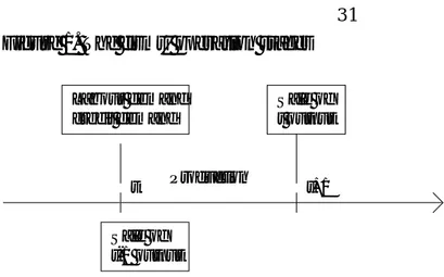
Let us consider an economy where firms produce competitively one single non-storable consumption good, called "the output" of the economy, by means of homogeneous labour and a decreasing-return technology. Absent physical capital, there is only private organization of production ("firm") in this economy, and each firm is run by a single manager who is entitled to profits and losses. All firms have the same operation cycle with two stages: production and sales. The production stage takes one discerete period indexed with t, regardless of the scale of output, while the sale stage takes place in t+1 and is virtually instantaneous. Therefore, at the beginning of each t all firms demand labour as a function of the output planned for sale in t+1, while they sell the output produced in t-1, and so on as in the chart below:

[Figure 1]

Unlike in traditional macroeconomics, in the class of models considered in this paper the time structure of transactions and the structure of contracts among economic agents are of great importance as they impinge upon the functioning of markets and of the whole economy. In particular, the time structure of transactions is such that firms need an amount of means of payment (at least) equal to their wage bill for each t. This requirement by firms, which disappears in standard macroeconomic models based on simultaneous transactions on all markets, is viewed as a key ingredient in the macroeconomics of credit (e.g. Blinder-Stiglitz, 1983; Blinder, 1987; Greenwald-Stiglitz, 1987).

In order to accommodate this factor in the model I posit the following characterizing assumptions:

(A1) There exists a general means of payment in the form of fiat money issued by a government agency called "the central bank". Interest-free money is the only asset in the economy.

(A2) Workers and firms stipulate "standard labour contracts", that is to say, contracts in terms of money which are resolved through payment by the end of the operation cycle. (A3) The central bank operates a credit window at the beginning of each t. Any borrower j receives the contractual amount of credit Bjt against his commitment to pay Bjt(1 + Rt) < Kjt in t+1, where Rt is the bank nominal interest rate and Kjt denotes the borrower's personal resources4.

(A1) and (A2) are implied by each another, and they can be taken to represent imperfect capital markets. In fact, one might design labour contracts like private securities and the wage rate as their price5, in which case (A1) and (A2) would drop together. The latter would be viewed as a case of perfect capital markets, with workers in a position of suppliers of firms' (working) capital. Hence (A1) and (A2) amount to assuming, loosely speaking, that firms are "fully rationed on the equity market" (see e.g. Greenwald-Stiglitz, 1990, 1993).

Under "full equity rationing", a firm may finance its wage bill either from internal funds or by borrowing on the credit market. (A3) states the credit conditions for those firms which resort to borrowing. The ensuing monetary regime is one where the central bank pegs the interest rate and the market determines the quantity of money supply, which is otherwise known as the "endogenous money" model (see e.g. Kaldor, 1982; Moore, 1988; King-Plosser, 1984)6.

In this economy, the firms resorting to credit face a bankruptcy risk impinging on the manager. Following (A3), if firm j borrows Bjt = (1 - θjt)StLjt, where θ is the self-financed fraction of the wage bill, St the contractual money wage rate, and Ljt the labour input, the manager's earnings scheme will be the following:

(A4) _St in t

Zjt+1 if Zjt+1 > 0

} in t+1 _{Zjt+1 -kjtBjt(1+Rt) if Zjt+1 < 0}

where Zjt+1 = Pjt+1Y(t)jt+1 - StLjt(1 + (1-θjt)Rt) is profit, Y(t)jt+1 is the output produced in t and sold in t+1, Pjt+1 is the selling price, Zjt+1 < 0 is a state of

4_{The borrower's personal resources cannot be traded directly for working capital, which is another} implication of imperfect capital markets. The fact that borrowing cannot exceed the borrower's personal resources ensures that the central bank bears no risk whatsoever.

5_{For instance, each worker in t receives from the hiring firm S}

t labour bonds for unit of labour services; each labour bond will be convertible into the consumption good in t+1 at the market price.

bankruptcy, and kjtBjt(1+Rt) is the incidence of the bankruptcy procedure on the manager's personal resources.

(A4) introduces bankruptcy risk into the firm's decision making as a consequence of "equity rationing". In fact, the manager is paid at the market price of labour, and then seizes the firm's whole profit, if positive, or deducts the firm's outstanding liability from his personal resources. In addition, the bankruptcy procedure typically entails costs that are assumed to be proportional to the value of the firm's debt7. Full payment of profits and interests also implies that the firm's revenue is always exhausted, so that θ_{jt = 0 for all j and t.}

We now need an explanation of why bankruptcy may occur, and possibly a probability measure of it. First of all, we are obviously not interested in situations where all firms either go bankrupt or make profits; in other words, we need an economy where firms may differ in their performance. Indeed, the heterogeneity of agents, as opposed to the representative agent methodology, is central to the new micro-and macroeconomics of credit micro-and bankruptcy (e.g. Greenwald-Stiglitz, 1987; Stiglitz, 1991). Heterogeneity may be introduced ex post -i.e. as (stochastic) differences in firms' realizations- or ex ante -i.e. as differences in firms' plans8. I shall follow this latter way, stressing an inherently informational aspect of bankruptcy risk through the following assumption:

(A4) Let all agents observe the vector of current market prices at any t. Henceforth, Pe(t)jt+1 and Pe(t)wt+1 will be the privately held expected output price of the firm j and of the worker w conditional on the public information available at t. Given a continuum of firms and workers, let ft(Pe(t)jt+1) and gt(Pe(t)wt+1) be the density functions of the expected prices across firms and workers, respectively.

(A5) Given ft(Pe(t)jt+1) and gt(Pe(t)wt+1), in each t there exists an average expected price in the economy Pe(t)t+1, conditional on the information available at t, i.e.

7 _{This personal component of costs is distinctive of the manager's liability in the firm due to debt finance} as opposed to a fully equity-financed firm, where k_jt > 0 (see Stiglitz, 1993). The Greenwald-Stiglitz macro-model, however, does not specify the debt contract between the manager and the bank and assumes a positive cost of bankruptcy as an increasing function in the firm's output. The authors put forward a number of justifications for this assumption, though perhaps the most important argument is that "having bankruptcy costs depend on [output] is necessary in order to ensure that the possibility of bankruptcy is never ignored" (p.89). (A4) shows that this may be the case with k_jt > 0. An alternative strategy would be to let the bankruptcy probability increase with output (see also Greenwald-Stiglitz (1993), p.86, and below, fn. 10).

8 _{The Greenwald-Stiglitz (1993) model is an example of the former type, since each firm ex post faces an} individual selling price which is a stochastic deviation from the output average market price. Therefore, it seems that an imperfect output market is also assumed. This additional imperfection is unnecessary if firms heterogeneity is introduced ex ante as shown above.

Pe(t)t+1 = =∞_∫P te( )_jt+1f P t_t( e( )_jt+1)dP te( )_jt+1=∞_∫P te( )_wt+ g P t_t( e( )_wt+ )dP te( )_wt+ 0 1 1 1 0 = Pt+1

(A4) amounts to introducing a partition between (homogeneous) public and (heteregeneous) private information. At this stage of analysis the causes of different expected prices are not important: thay can be thought of as a product of genuine heterogeneous beliefs on the economy, or as the result of whatever firm-specific computation or measurement error. The individual expected price is also representative of the firm's project (in a competitive market, with a decreasing-return technology there is a one-to-one map from the expected price to the optimal planned output), so that we may also say that each firm's project is not observable ex ante either9. (A5) states that the average expectation of firms and workers is the same, and that it turns out to coincide with the actual price.The first part is only a simplifying assumption that prevents phenomena that may arise at the aggregate level from introducing further differences in the average expected price of firms and workers. Though potentially interesting, these phenomena fall outside the scope of the present paper. The second part amounts to a "population's rational expectations hypothesis", in the sense that price expectations are "on average correct", where the average is taken across the population of agents. This hypothesis is held in order to focus on the role of heterogeneity of expectations at the individual level, though it is admitted that the population of agents cannot be systematically wrong as a whole.10

9_{This partition between public and private information is now common in models of heterogeneous} information; moreover, the existence, at least ex ante, of private, unobservable information should be understood as a typical feature of competitive markets where all agents are "small" and ignore each other. On this issue see also Pesaran (1987, ch.2).

10_{Assumptions (A4) and (A5) give a representation of the price expectations economy-wide which seems} close in its substance to the evidence reported by major studies on business surveys. Carlson-Parkin (1975) in their path-breaking work on measuring inflation expectations from business surveys introduced the practice of assuming individual expectations in the economy to be distributed according to a given density function (they also assumed that each individual has his/her own distribution from which his/her responses are drawn, but this further assumption would only complicate our setup). Visco (1984), examining the opinion poll of the Italian magazine Mondo Economico, and Pesaran (1987, ch.8), using the data from the business survey of the Confederation of British Industries, both applied the same methodology under alternative specifications of the hypothetical density functions of expectations. The Mondo Economico opinion poll is elaborated jointly with the Italian official Institute for Conjunctural Analysis (ISCO), whose methodology is again based on the assumption of distributed expectations in the economy (see D'Elia, 1991). The tendency of price expectations to be "correct on average" was found by Visco, though limitedly to the period before the oil shocks of the 1970s. Pesaran instead rejected the "populations's rational expectations hypothesis".

Given (A3) and (A4), a bankruptcy state of firm j occurs whenever it defaults on its bank debt, i.e. when Pjt+1 < Vjt, where Vjt = StLjt(1 + Rt)/Y(t)jt+1 is the average cost of producing Y(t)jt+1. Given that Pe(t)jt+1 > min(Vjt+1) is the market entry condition, bankruptcy occurs if the firm's expected price turns out to be higher than the actual output price, and the actual output price is lower than the firm's average cost. In particular, let

Φ_jt ≡ _{Prob(Pjt+1 < Vjt)}

be the probability of the default state for the firm, and φ_{jt its estimated value by the} firm. Therefore, kjtStLjt(1 + Rt)φjt is the manager's expected bankruptcy cost.

2. Individual plans

2.1. Firms

It is assumed that managers are risk-neutral and wish to maximize earnings over their plain wage. Given the above time structure of production and transactions, however, a manager has to plan production in period t whereas sales and profit will materialize in period t+1. From (A4) and (A5), the j-th manager's expected earnings as of t will be11:

(2.1) _{E(t)jt+1 = St + [Pe(t)jt+1Y(t)jt+1 - StLjt(1 + Rt)(1 + kj}φ_jt)] Hence, the firm's programme is:

(2.2) _{maxL E(t)jt+1}

given the production function (2.3) _{Y(t)jt+1 = L}η_jt for all firms, with 0 < η < 1.

As usual, it is convenient to compute the log-linear solution of the firm's programme, which yields the following labour demand function (unless otherwise stated, the log of each variable will be denoted by converting the notation from capital to small-case letters): (2.4) _{ljt = d - g(}ϕjt + st + rt - pe(t)jt+1) with δ η η γ η ϕ φ = − = − = + = + log , , log( ), log( ) 1 1 1 jt 1 kjt jt rt 1 Rt

Equation (2.4) displays some typical features of the models of firm with credit (e.g. Greenwald-Stiglitz, 1990, 1993). First, because of the time lag between production

and sale, the firm's employment decision is ruled by its expected real marginal cost (the term in brackets), not the current one. Second, the real marginal cost includes the bank interest rate rt and the expected bankruptcy cost ϕjt ∈ [0, ∞], bankruptcy risk for short, which increases as φ_{jt or kjt increase. That is to say, an increase in the estimated default} probability or in personal bankruptcy costs induces the manager to reduce employment and output. On the other hand, (2.4) becomes the standard labour demand function when rt = 0, φjt = 0 or kjt = 0.

From (2.4) we see that the individual labour demand may differ according to the firm's expected price and bankruptcy risk. It will be convenient to work with average functions as representative of the market. To this effect we can exploit (A5) to obtain (2.5) _{ldt = d - g(}ϕt + st + rt - pe(t)t+1)

where pe(t)t+1= logPe(t)t+1, and ϕt is the average value of the individual estimations of the bankruptcy risk.

2.2. Workers

Workers are assumed to choose rationally between leisure and consumption in a competitive labour market. I shall adapt to the present context the general life-cycle choice model elaborated by Lucas-Rapping (1969) and Sargent (1979), where a worker w at any t is characterized by an individual system of preferences over the quantity of leisure Hwt and of consumption Ywt in t and onwards, represented by the utility function

(2.6) _{Ut(Hwt, Ywt, ...)}

for all w, monotonically increasing and twice differentiable in each argument, with Hwt Î [0, H] and H as the social maximum working time.

Given the structure of transactions in the economy, the worker at the beginning of time t observes the current price of output Pt, the contract money wage St and forms the expected output price Pewt+1. Then he should choose how much labour to sell in period t, and how to distribute his period-t labour income between t, when output produced in t-1 is available, and t+1, when output produced in t will be available, knowing that interest-free money is the only asset in the economy. The resulting utility maximization problem is:

maxH,Y Ut(Hwt, Cwt, Cwt+1) subject to

(2.7b) _{PtCwt + Mwt = StLwt}

(2.7c) _{Pewt+1Cwt+1 < Mwt}

where Lwt is labour supply in t, Mwt are money balances, and Cwt , Cwt+1 is consumption in t and t+1.

Under the usual assumptions that leisure and consumption are nomal goods and that an internal solution exists, the Lucas-Rapping-Sargent model yields:

(2.8a) _{Lwt = Lw(St/Pt, P}e_wt+1/Pt) (2.8b) _{Cwt = Yw(St/Pt, P}e_wt+1/Pt)

(2.8c) _{Cwt+1 = Mwt/Pt+1}

with L'w1 > 0, L'w2 < 0, C'w1 > 0, C'w2 < 0. Note that Pewt+1/Pt is 1 + the expected inflation rate (expected inflation rate for short).

The worker's choice between leisure and consumption and between present and future consumption is ruled by the current real wage rate and the expected inflation rate. But the cross-elasticity between present leisure and future consumption is not nil: an increase in Pe_{wt+1 which raises P}e_{wt+1/Pt amounts to a fall in St/P}e_{wt+1, the} expected real wage rate, hence Ls_{wt is decreasing in P}e_{wt+1/Pt or else increasing in} St/Pewt+1.

Again following Lucas-Rapping and Sargent we may also assume that a log-linear specification of (2.8a) exists and is the following:

(2.9) _{lwt = a + b1(st - pt) - b2qe(t)wt+1}

where qe(t)wt+1 = pe(t)wt+1 - pt is w's expected inflation.

According to (2.9), the individual labour supply may differ in the expected inflation. Using assumption (A5) as in the case of firms, we may obtain the average labour supply as representative of the whole market:

(2.10) _{lst = a + b1(st - pt) - b2qe(t)t+1}

where qe(t)t+1 = pe(t)t+1 - pt is the economy's average expected inflation

3. Heterogeneous expectations, bankruptcy risk and macroeconomic equilibrium

In the following parts of the paper I shall focus on the role of credit and bankruptcy risk in determining the economy's macroeconomic outcomes. In particular, I shall use this model economy to show that heterogeneous price expectations may be the source of bankruptcy risk. Later in section 4 I shall discuss whether this kind of heterogeneity may persist or not.

3.1. Macroeconomic equilibrium

First, recall that at the beginning of each new operation cycle t, the markets for labour and credit determine the nominal wage rate st, the level of employment lt, and the amount of credit lent to firms bt, given the current output price pt, the bank nominal interest rate rt, the average bankruptcy risk ϕt, and the average expected price pe(t)t+1. The labour demand and supply functions are those obtained in section 2 (2.5), (2.10), and hence the labour market equation is

(3.1) d - g(ϕt + st + rt - pe(t)t+1) = a + b1(st - pt) - b2qe(t)t+1

The amount of credit is demand determined and is simply equal to the economy's wage bill,

(3.2) _{bt = st + lt}

which also corresponds to the period's money supply.

Subsequently, in the next period t+1 all firms can sell their output, and the output market determines the equilibrium price. Output supply is

(3.3) _{y(t)t+1 =} η_lt,

an amount fixed and non-storable. Output demand is given by equation (2.8c) in the workers' optimization programme, that is, ct+1 = mt - pt+1 for all workers. Since mt = bt = st + lt, the output market equation is

(3.4) η_{lt = st + lt - pt+1}

Under "population's rational expectations" according to (A5), the equilibrium solutions of equations (3.1)-(3.4) for the real wage rate, ω_{t = st - pt, the real money} supply, µ_{t = bt - pt , the level of output, y(t)t+1, and the inflation rate, qt+1 = pt+1 - pt,} are the following:

[

]

( . ) ( . ) ( . ) ( . ) ( ) ? ? 3 5 3 5 3 5 3 5 1 1 0 0 0 0 1 1 1 1 a b c d y t q y q y q r t t t t t t ω µ ω µ ω µ ϕ + + − −             =             +                   +

(the coefficients display their sign underneath; their values are specified in the Appendix; the intercepts, denoted with 'o' are omitted for brevity).

3.2. Credit, bankruptcy risk and output

The macroeconomic equilibrium is determined by two "financial variables", the bankruptcy risk ϕ_{t, as estimated on average by firms, and the nominal interest rate rt,} fixed by the central bank. We can first draw the following proposition concerning the relationship between credit, bakruptcy risk and economic activity.

(P1) The level of output is decreasing in the estimated bankruptcy risk and in the nominal interest rate if β_{1 >} β_{2 (see Appendix)}

(P1) can be interpreted as a non-neutrality proposition which is common to other macroeconomic models of imperfect capital markets (see e.g. Greenwald-Stiglitz, 1988a, 1988b, 1990)12. Note, however, that this result is conditional on the relative magnitude of the parameters of the labour supply function. The condition β_{1 >} β₂ reflects a sufficiently low intertemporal substitution effect, that is to say, labour supply reacts more to changes in the current real wage than to changes in expected inflation13. If this condition is met, the reason behind (P1) is simply that both financial variables affect the real marginal cost of firms at a given expected price. To focus on the role of the bankruptcy risk, suppose that ϕ_{t rises. Ceteris paribus, the expected real marginal} cost for firms rises too, and labour demand falls. Since it is assumed that workers and firms on average correctly anticipate the deflationary impact of ϕ_{t, this tends to lower} the nominal wage rate and the real marginal cost for firms. This exerts a positive counter-effect on labour demand, which is stronger the greater is β_{2, and vice-versa. In} any case, it is certainly significant that the non-neutrality of the financial variables may result, through the interest rate and the bankruptcy risk, even though price expectations are (on average) correct, and markets are perfectly competitive14.

On empirical grounds, as is clear from equation (3.5c), ϕ_{t lends itself to} straightforward interpretation as a source of aggregate supply shocks alternative to the

12_{However, it should be clear that (P1) does not imply per se that there may be involuntary} unemployment (the labour market does clear, the nominal and real wage rate being negative elastic to changes in those same variables).

13_{In fact, Greenwald-Stiglitz (1993) obtain that output is always decreasing in the bankruptcy risk} because they model labour supply as a function of the current real wage only, which is equivalent β₂ = 0 in the present model. On the other hand, the well-known full-neutrality result of the new classical theory obtains if β₁ = β₂, which yields the typical labour supply function depending on the expected real wage only. There seems to be no reason why one should subscribe to either of the two extreme versions of the labour supply function.

14_{Thus, another idea of Keynes's (1936, ch. 19), that the mere downward flexibility of wages and prices} could generate no increase in employment and output, finds substantial support from consideration of firms' liabilities and bankruptcy risk (e.g. Greenwald-Stiglitz, 1987). This issue, too, is not at all new in the macroeconomic debate since it dates back to Fisher's theory of debt deflation: see e.g. Tobin (1980), and Minsky (1982).

technology/tastes shocks preferred in the new-classical camp (Greenwald-Stiglitz, 1987, 1990, 1993; Gertler, 1988; Bernanke-Gertler, 1987). Shifts in aggregate supply originating in yo or in ϕt would hardly be distinguishable on empirical grounds. Yet some argue that technology/tastes shocks of the magnitude required to reproduce the observed swings in output strain credibility, whereas the bankruptcy risk perceived by firms is typically volatile. Last but not least, this factor is reminiscent of Keynes's original view that business fluctuations are rooted in the instability of the entrepreneurs' state of confidence (Greenwald-Stiglitz, 1987)15.

3.3. Expected prices and the bankruptcy mechanism

So far, we have examined the macroeconomic consequences of firms' fallibility and their related bankruptcy cost assuming that each firm has its own estimation of its default probability on which the individual bankruptcy risk ϕ_{jt is built. We have seen in} section 2.1 that the individual estimation of the default probability is based on the firm's understanding that the actual output price may turn out to be lower than its expected price Pe(t)jt+1 and lower than the average cost of the output level associated with Pe(t)jt+1. Now, in the light of the macroeconomic results obtained above, we will be able to examine the bankruptcy mechanism in detail revealing its systemic nature, that is to say, the fact that the default probability of each single firm depends on the expected prices distribution in the whole population of firms.

First, recall that the macroeconomic results in system (3.1) are in fact average market values, as if they were produced by the interaction between the "average firm" and the "average worker" representative of the respective populations. As can be checked in equation (3.4), the process of endogenous money creation in the economy is such that the actual output price Pt+1 is always equal to the average cost of producing Y(t)t+1; hence, the "average firm", whose expected price coincides with the actual price, makes neither profits nor losses - which is consistent with the free-entry assumption of the model. Consequently, the defaulting firms are those that have produced at an average cost greater than the "average firm's". Since all firms are equal

15_{Of course, in Keynes's view changes in the entrepreneurs' state of confidence are responsible for} aggregate demand instability. The shift of focus of this class of models from demand to supply is theoretically and empirically important. The present model shows that the elasticity of output to the "financial factors" is proportional to its elasticity to labour inputs h and to the elasticities of labour supply b₁and b₂. The claim that this transmission mechanism from credit cost to output supply is likely to be much stronger than the old-Keynesian one going through asset prices and the asset-prices elasticity of output demand appears largely an empirical matter.

except in their expected price, it also the case that the defaulting firms are those with expected price i) higher than the population's average, and ii) higher than the marginal cost of the "average firm". Therefore, whereas the average profit in the economy is always zero, heterogeneous price expectations entail that it is always possible to sort out three classes of firms so that

(1) _{Pe(t)jt+1 < Pe(t)t+1 = Pt+1, Zjt+1 > Zejt+1 > 0 [high profits]} (2) _{Pe(t)t+1 < Pe(t)jt+1 <} Pe( )t _t+1 0 < Zjt+1 < Zejt+1 [low profits]

(3) _{Pe(t)jt+1 >} Pe( )t _t+1, Zjt+1 < 0 [default] where Pe( )t _t+1 is the expected price coincident with the marginal cost of the "average firm".

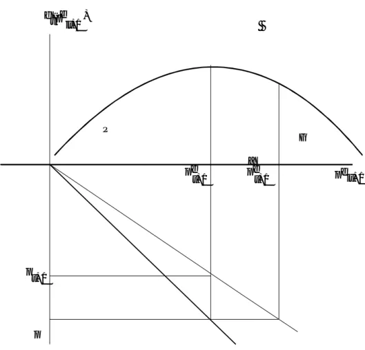
The first class makes "high profits" in the sense that actual profits exceed the expected ones. The second class makes positive profits, but lower than expected. The third makes negative profits and defaults. This result can be better understood with the help of figure 2, which represents the usual price-cost-output plane for the individual firm and shows the three classes where the firm may fall at t+1 according to its own expected-price-output choice at t

[Figure 2]

Point A denotes the "average firm's" expected-price-output combination. All firms whose expected price exceeds Pe( )t _t+1 will produce at their marginal cost to the right of Y(t)t+1, i.e. with an average cost greater than at point A and hence greater than the actual price Pt+1, so that they will default.

Knowing the density function of expected prices in assumption (A5), ft(Pe(t)jt+1), we can give a probability measure to each single class of firms:

Probability of class 1: Probability of class 3: Probability of class 2: Π Γ Π Γ t t e jt e jt Pe t t t t e jt e jt P t t t t f P t dP t f P t dP t - -= = + + + + + − + ∞

∫

∫

( ( ) ) ( ) ( ( ) ) ( ) ( ) ( ) 1 1 0 1 1 1 1 1

Therefore, the following proposition holds:

(P2) The individual default probability, understood by the firm as the probability that the actual price falls below its own average cost, Φ_jt ≡ _{Prob(Pjt+1 < Vjt), is in fact} given by Γ_t ≡ _{Prob(Pe(t)jt+1 >} Pe( )t _t+1) for all j. Hence it depends on the distribution of expected prices in the population.

Let us now examine in greater detail how the characteristics of the distribution of expected prices in the economy affect the default probability in the economy. In particular, let us focus on the first two moments of the distribution. First of all, it should be noted that the threshold value of bankruptcy Pe( )t _t+1 is itself a function of the mean value of the distribution. In fact, Pe( )t _t+1 is the marginal cost of producing the economy's optimal (average) ouput Y(t)t+1; hence we can write Pe( )t _{t+1(Y(t)t+1),} with ∂Pe( )t _t+1/∂_{Y(t)t+1 > 0. As can be deduced from equations (2.1)-(2.3), Y(t)t+1 is} in turn an increasing function of the average expected price Y(t)t+1(Pe(t)t+1), ∂ Y(t)t+1/∂Pe(t)t+1 > 0. Consequently, it should be that Pe( )t _{t+1(Pe(t)t+1), with} ∂

Pe( )t _t+1/∂Pe(t)t+1 > 0. In particular, equations (2.1)-(2.3) yield the linear function: (3.5) Pe( )t _t+1 = Pe(t)t+1/η2

This relationship, with its feedback on the default probability, is reproduced in figure 3 for a hypothetical unimodal symmetric distribution.

[Figure 3]

Figure 3 highlights how the first two moments of the distribution determine Pe( )t _t+1 and the default probability in the economy. First, consider the mean value Pe(t)t+1: an increase in Pe(t)t+1 associated with a parametric shift of the whole distribution to the right increases Pe( )t _t+1. Since Pe( )t _t+1 increases more than Pe(t)t+1, and the probability mass is left unchanged, the new default probability should be smaller. Second, consider the variance of the distribution: a mean preserving spread of the distribution that increases its variance determines a larger default probability. Hence we may add the following new proposition:

(P3) The default probability in the economy decreases with the mean value, and increases with the variance (mean preserving spread), of the distribution of the expected prices in the firms' population.

Propositions (P2) and (P3) have several other implications that are worth emphasizing. First, the above shows that heterogeneity of expectations is sufficient for firms to face a positive probability of default even though firms are technically identical and the price-generating process is deterministic. Default is, in this setup, simply a matter of relative expected prices. The dependence of the default probability on the characteristics of the distribution of expected prices in (P3) may pinpoint some popular

views among businessmen, reflected in short-term business surveys and forecasts, such as the view that a buoyant market with rising prices is less severe for profitability16, or the view that greater uncertainty (heterogeneity) may bring about more mistakes and losses17.

Second, on methodological grounds the most important consequence of considering heterogeneity behind "average behaviour" is that the usual argument that the economy as a whole cannot be systematically wrong cannot be stretched to justify the short-cut of assuming a perfectly informed representative agent. In fact, we have seen that although the firms' population on average may have the correct price expectation, each single firm may fail and should discount a bankruptcy risk, whereas the "representative firm" in the standard methodology, anticipating the correct output price, would not. Hence, the average estimated bankruptcy risk by firms appears in the macroeconomic equilibrium values in system (3.1), whereas the standard methodology would induce us to ignore it.

Third, another important methodological problem arises in connection with the correct estimation of the default probability by the single firm. Statistically, this is a problem analogous to the computation of the rational expectation of a stochastic variable in that the agent is required to know the distribution of the variable. There are also significant differences. The first is that in our case the agent should know the first two moments of the distribution18, whereas in standard rational expectations computations only the first moment is necessary. The second difference is that the relevant variable is the expected price by the other agents, not directly a market realization. The third is that as soon as the distribution of expected prices in the economy became common knowledge, the bankruptcy mechanism would vanish, since every firm would discover the average expected price. In othe words, a typical "beauty

16_{The literature on the negative effects of Fisher's "debt deflation" is also to be metioned here, with its} central message that inflation is beneficial to debtors. Generally, analyses in this vein focus on the stock of outstanding debt, whereas I have focused on the default probability. Following the seminal works by Minsky (1982), an explicit role for the debt stock can be found in the contributions of Bernanke (1983), Bernanke-Gertler (1987), Greenwald-Stiglitz (1993).

17 _{A well-known piece of evidence shows that the variance of the price level increases with the inflation} rate. To the extent that this phenomenon is reflected in the degree of heterogeneity of price expectations, the positive effect of inflation in reducing bankruptcies may be dampened. Visco's (1984, pp. 57 ff.) analysis of the Mondo Economico opinion poll detects a high degree of correlation (ranging from 0.67 to 0.8 under different measures) between upward inflation expectations and increase in their variance in the population after the first oil shock. As Visco himself suggests, rising inflation alone may not be the cause of increased uncertainty, unless this is perceived as a structural change in the economy.

18_{As explained above, the default probability Γ}

t comes to depend on the mean and variance of the distribution of expected prices in the economy.

contest" problem is involved19, and the key question is whether each single firm has access to the relevant information or not. Assumption (A4) introduced a distinction between public, freely observable, information, and private, non observable, information. This partition of information, which is basic to all models of heterogeneity, implies in our setup that the single firm is prevented from collecting all the information necessary to compute the distribution of expected prices with its characteristics. Thus the bankruptcy mechanism hinges on limitedly informed firms, which does not mean that they behave irrationally.

The present model provides an example of this general principle. Given available information at the individual level, each profit-maximizing firm understands that it should discount a bankruptcy risk due to its own default probability, i.e. the probability Φ_{jt that the market output price falls below its own average cost. Let us call} this "atomistic information". However, the fact that the default event will occur if the firm's expected price exceeds the threshold value Pe( )t _t+1, or that Φ_{jt =} Γ_{t, is} completely hidden from its view. For this fact is the consequence of the whole economy's aggregative activity of the heterogeneous plans of the firms that generates the Pe( )t _{t+1(Pe(t)t+1) relationship reproduced in figure 320. Let us call this "systemic} information". At this point one may envisage two different theoretical routes. The first is the one we have followed so far, that is, each firm only has "atomistic information", proceeds on the basis of its own estimated value φ_{jt of} Φ_{jt, and the macroeconomic} equilibrium results reflect the average estimated bankruptcy risk ϕ_{t as in system (3.1).} The second assumes that, perhaps by chance, the estimated value φ_{jt by each firm turns} out to be equal to the correct Γ_{t for all firms, which yields the "true" bankruptcy risk} measure to be placed in system (3.1). The two routes lead qualitatively to the same result. In no case, however, can we assume that each firm is endowed with "systemic information", unless we explain how private information is made freely observable in the economy.

19_{A "beauty contest" problem arises whenever the rational choice of an agent depends on his knoweldge} of the choices made by all the others. As is well-known this term goes back to Keynes's analysis of stock market traders in chapter 12 of the General Theory. This kind of problem arises whenever a system is "self-referential", that is to say, when the system's states depend on the collective anticipation of them. The modern treatment of this class of problems, in the context of expectations formation, can be found in Pesaran (1987, ch.4) and Sargent (1993).

20_{Hence, some would probably label these firms as "boundedly rational", since they are not only limitedly} informed about the economy's parameters set, but they also have limited understanding of the process that generates the relevant market outcomes. On this point see again Pesaran (1987, ch.3).

4. Can firms discover the bankruptcy mechanism?

The bankruptcy mechanism in-built in the present model is exclusively informational, in that it originates from the limited "atomistic information" available to firms, which prevents them from computing the distribution of expected prices in the whole population. A natural question at this point is: How information-tight is the bankruptcy mechanism? And, consequently, how persistent is the heterogeneity of price expectations?21

To address these issues we should first of all examine how much "systemic information" can be obtained by each single firm. In principle we know that information can accrue to an individual i) through the individual's activity (which leads to enlarging one's private information), or ii) through the activity of a collective device or institution (which makes information a public good). A typical example of activity i) is learning by doing, and of activity ii) the market or public economic agencies. Moreover, the two informational sources can interact, with e.g. public agencies helping individuals to learn through their market activity. Though at present I am unable to add a detailed model of information acquisition to the model of section 3, in this section I shall explore its potential role and consequences under three basic points: i) existence and stability of the rational expectation of the inflation rate, ii) incentives to learn, iii) interaction between learning and bankruptcy.

4.1. Learning through the market

An intriguing feature of the bankruptcy mechanism of section 3 is that the "atomistic information" at firms' hands is not wrong, it is simply spurious. Indeed, a firm's ability to reduce its default probability need not result from a correct understanding of the existence of the threshold expected price Pe( )t _t+1, but more simply from its accuracy in forecasting the actual output price. This is also perhaps the more natural way a manager may perceive the problem. Therefore, an apparently obvious point to start from seems to examine whether a firm can learn to infer the correct value of qt+1 from the information available at t. However, the problem of individual learning, the ability of a single firm to approach the "average firm" in a large population, is almost irrelevant. The truly relevant problem is whether the whole

21_{If one looks at the evidence coming from business surveys recalled in the Introduction, one should} rather rephrase the above question asking why the heterogeneity is persistent.

population of firms can, through learning, collapse onto the "average firm's" expectation. Yet we should also be aware that changes in the population's expectations have macroeconomic effects. This is a key issue as far as learning is concerned.

In the model of section 3 it was assumed that the population of firms on average has the correct expectation of the inflation rate. System (3.5) resulted from solving the demand-supply equations (3.1)-(3.4) for qe(t)t+1 = q(t)t+1. The inflation equation (3.5d), in particular, resulted from

(4.1) _{qt+1 = q'0 - q''1(rt -} ϕt) + q'1qe(t)t+1 with q''1 = [1 + β1(1 - η)]-1.

This equation shows that, as long as the "population's rational expectation" is not established, the actual inflation rate depends on its average expectation in the economy. In other words, the economy under examination is a "self-referential system"22. A system of this kind raises thorny problems as to expectations formation and learning, on cognitive, theoretical and empirical grounds.

The first step is to assess the existence of a rational expectations solution for equation (4.1), i.e. a solution for qe(t)t+1 = q(t)t+1. This solution exists and has already been given in equation (3.1d). Technically, this solution procedure amounts to finding the fixed point of the map qe(t)t+1 → q(t)t+1. In a learning problem, however, the sole existence of the fixed point is not sufficient. Suppose the firms' population starts far away from the fixed point: since learning is intriniscally a dynamic phenomenon, we need the fixed point to be an "attractor" in the map qe(t)t+1 → q(t)t+1, or in other words, to be dynamically stable.

This second step of analysis is particularly hard because it is necessary to introduce a motion law of qe(t)t+1. The standard line of argument is as follows. As long as qe(t)t+1does not coincide with qt+1, there must operate a revision rule of qe(t)t+1. This rule is generally assumed to be a map I(t) → _{qe(t)t+1, where I(t) is the information} set available at t.

The motion law of qe(t)t+1 is nothing but a representation of the learning process in the economy. An interesting, albeit uncomfortable, feature of the state of the art is that there exist many conceivable learning processes. On the other hand, the modeller's choice is bounded by two criteria: rationality and/or cognitive capacity. Ongoing research in post rational-expectations economics revolves around the mutual consistency and interaction of these two criteria. Those who particularly stress rationality assume learning processes based on statistic methods, such as bayesian learning, least squares learning, etc. (see the works surveyed by Pesaran, 1987, ch.3;

Sargent, 1993). Those who are concerned with the cognitive feasibility of learning processes instead draw on cognitive tools such as genetic algorithms, classifier systems, neural networks (Arthur, 1991; Miller-Holland, 1991; Moss-Rae, 1992; Sargent, 1993).

One of the simplest examples of learning process is the case of homogeneous "static expectations", i.e.

(4.2) _{qe(t)jt+1 = qt, all j}

This is a special case in which I(t): {_qt}_{. Consequently, one obtains a dynamic map qt} → _{qt+1, whose stable steady state values also ensure convergence and stability of the} motion law of qe(t)t+1. In fact, substitution of this equation into (4.1) leads to a first-order linear difference equation for qt+1. Since q'1 < 1, we can say the following:

(P4) If qe(t)t+1 = qt, the learning procees is convergent and stable for any intial value qe(t)t+1 ≠ qt+1.

Though based on a very specific, and arbitrary, assumption, the resulting dynamics of inflation contains a typical feature of economies under learning processes, namely that the learning process itself modifies the macroeconomic results. In the mind of the economy's creator there is no structural relationship between qt+1 and qt, nor is there a dynamic adjustment process to inflationary shocks. Learning by itself may create such a relationship, and once it is established it would be irrational to ignore it.

However, P4 is far from conclusive. From both the rationalist and cognitive viewpoints, the case of static expectations is seriously limited. Unless the relevant variable follows a pure random walk, static expectations ignore information that can be contained in contemporaneus variables that co-determine the relevant future variable23. This is exactly the case of equation (4.1), which contains at least one freely observable variable, the interest rate rt , to which qt+1 is correlated. The class of "boundedly rational" learning models (Pesaran, 1987, ch.3) assumes that agents exploit all available public information contained in reduced-form equations of relevant variables in order to form and revise expectations on these variables, according to recursive least-squares estimations. In our case, at any time t, given the information set I(t): {_{qt-τ, rt-τ}}, with τ = 0, 1, ..., for all firms, the equation to be estimated by each firm, taken from (4.1), is:

23_{In the cognitive approach, human beings draw expectations from "mental models", which are} representations of relationships between "objects" based on experience. There is close affinity between this view, and the idea of agents as "economic modellers" popularized by the rational-expectations school. The two schools differ sharply as to the content, extension and elaboration of mental models, and in particular the cognitive school denies that mental models can ever be an isomorphic representation of "reality" - whatever this word means (Tamborini, 1997). Beltrametti et al. (1996) have shown that a classifier system - one of the most powerful learning computer-models based on the cognitive principle of mental models - is indeed able to exploit information on exchange-rate theoretical "fundamentals" to predict exchange-rate changes profitably, whereas most statistical studies do not reject the random-walk hypothesis and thus lead to ignore fundamental variables.

(4.3) _{qt+1 = q'0 - q'1rt +} ε_t which yields

( . )4 4 qe t( )_t+1=q t~ ( ) ~ ( )₀ −_{q t rt1}

where (∼) denotes OLS estimators at t. Substituting (4.4) into (4.1) we obtain the new inflation equation:

(4.5) _{qt+1 = q0(t) - q1(t)rt - q'1}ϕ_t

where q(t)0= q'0 + q'1q t~( )_{0, q(t)1 = q'1(1 +}q t~( )₁).

Let us note the following two essential features of least-squares learning. First, as already stressed, the learning process alters the inflation equation: the parameters in equation (4.5) have a time index and, generally, differ from the structural ones in equation (3.1d). Moreover, this alteration is a cumulative process, since the data generated by the inflation equation (4.5) will feed new estimated parameters in t+1, which in turn will alter the inflation equation for t+2, and so on and so forth. Second, the estimation equation (4.3) mistakes the unknown variables ϕt and qe(t)t+1 as a stochastic error term, which leads to inconsistent estimated parameters. The forecast error implied by the above estimation procedure is:

(4.6) _{qe(t)t+1 - qt+1 = [}q t~ ( )_{0 (1-q'1) - q'0] + [}q t~ ( )_{1 (1-q'1) - q'1]rt + q'1}ϕ_t which is not orthogonal. Moreover, the fact that in this case two unknown variables are missing from the public information set prevents firms from inferring them through error analysis. This reassures us that the problem for each firm to discover qe(t)t+1 is not trivial.

In spite of the above limitations, "boundedly rational" least-squares learning may still be "successful", in the sense that forecast errors may tend to become smaller and smaller through time (weak convergence). In our case, this occurs if

limt→∞q t~ ( )_{0 = q'0/(1-q'1), limt→∞}q t~ ( )_{1 = q'1/(1-q'1)}

which also implies limt→∞ϕt = 0. Yet, from (3.5d), it is easy to see that q'0/(1-q'0)= q0, and q'1/(1-q'1) = q1, that is to say, if the learning process displays weak convergence, it also converges to the structural parameters of the inflation equation (3.5d) and is therefore consistent with the rational expectations equilibrium (strong convergence). Note that this may not be necessarily the case: the learning process might not converge at all, or it might converge to parameters that are (permanently) modified with respect to the structural ones. Which of the three outcomes will prevail crucially

depends on the estimation and revision procedure that generates the sequence of estimated parameters24.

4.2. Learning in a heterogeneous population

Introducing heterogeneity and bankruptcy poses supplementary problems. First of all, one faces the usual aggregation problem. As is the case in equation (4.1), the actual inflation rate depends on the average expected inflation rate in the economy, whereas individual expectations are distributed around the latter. We cannot simply assume a law of motion of qe(t)t+1 as if this were a value held by all firms and all firms adopted exactly the same learning process, otherwise for any qe(t)t+1 > qt+1 all firms would go bankrupt25. Thus we should examine learning in a heterogeneous population, where individual differences around the average forecast can persist.

If we accept the simplifying assumption that firms adopt the same learning process represented by the least-squares estimation procedure presented above, it is not difficult to transform the estimated equation (4.4) from a single-valued forecast into a distribution of individual forecasts, in line with our previous assumption (A5) in section 2, provided that we also assume that each firm introduces an individual element, whether in the estimated parameters or as an additive disturbance. Admittedly, this is a rather ad hoc way to obtain heterogeneity in the learning process. However, if we are ready to admit heterogeneity at least as a feature of a less-than-perfectly informed population, heterogeneity may then be self-reproducing over time through the distribution mechanism of profits and losses that we have examined in section 326.

As we saw there, heterogeneity causes some firms in the population to obtain higher profits than expected, some firms to obtain lower profits than expected, and some to default. As a consequence, not all firms have the same pressure to revise their forecasts. It can be argued that the typical "learning agent" in standard learning models coincides with the firms in the second class only, that is, with only a part of the whole

24_{A detailed discussion of different estimation methods can be found in Pesaran (1987) and Sargent} (1993). The problem of convergence of learning to rational expectations equilibria is discussed in a general framework by Bray-Kreps (1986).

25_{This seems to be a general problem: as far as I know, learning models ignore the costs of errors, ignore} the actions that rational agents should take to protect themselves against errors, and ignore that errors can be fatal (economically) to an agent (see also Tamborini, 1997).

26_{If, during the learning process, the average expected price does not coincide with the acutal price, the} distribution of profits and losses results to be different quantitatively, but the bankruptcy mechanism remains the same as explained in section 3.

population. In principle, the firms in the first class, too, should be incentivated to forecast better, because their expected price turns out be lower than the actual one and hence their output is inefficiently low. However, it should be recalled that the distribution mechanism of profits and losses in the economy is such that as a firm approaches the "average firm's" correct forecast, profits shrink towards the zero average profit condition. Hence, the firms in the first class may have little, if any, incentive to change their forecasts27. As to the defaulting firms, the problem is simply whether they will have another chance or not. In the present simplified setup they will not, which implies that at the end of each period t, the population of firms changes its structure of cumulated information, in the sense that the information embodied in the defaulting firms dies out. This of course remains true also in a more realistic economy where only some defaulting firms actually go bankrupt. Since the thrust of learning models is the cumulation of information, as exemplified above, the critical consequence of bankruptcies is that they destroy information in the population as a whole. We can safely ignore this problem only if some informational device exists that freely transmits the information owned by the defaulting firms to the entering ones. Otherwise, the latter's forecasts will change the distribution of expected prices in the population. Thus, the different attitudes towards learning of the firms in the different classes, and possibly the structural changes in the distribution of expected prices due to the turnover of firms, may justify the persistence of heterogeneity in the population - and perhaps may make the idea of homogeneity less justifiable.

The eventuality of bankruptcy in a learning population, and the consequent injection of "less learned" newcomers, can also be linked to the research line on heterogeneity of Haltiwanger and Waldman (1985, 1989), which may shed light on the implied structural change in the distribution of expected prices. Their works investigate the aggregate consequences of agents' different abilities to obtain and process information. They usually partition the population in two simple classes - the "sophisticated" and the "naive" - and examine under what conditions the latter are able to alter the aggregate equilibrium outcome with respect to what it would be if all agents were sophisticated. The learning process depicted above quite naturally reproduces, in any period t of the process, the Haltiwanger-Waldman partition of the population of

27_{In a paper examining the performance of professional exchange-rate forecast services, Bilson (1983)} deals with a similar problem, which is known as "the right side of the market problem". In valuing forecast services, the customers are not interested in the precision of the forecast, but in its profitability. A small forecast error with the wrong sign (e.g. leading to a long position in foreign exchanges when the exchange rate instead appreciates) produces a loss, whereas a larger error with the right sign yields a gain anyway.

firms. Suppose that all firms adopt the learning process described by equations (4.3)-(4.4) up to an individual "white-noise" uncorrelated component. Consequently, in each period t there exists a distribution of expected prices in the population of firms such that in the next period t+1 a share Γ_{t of the population goes bankrupt as explained in section} 3. Each period t, therefore, is characterized by a class of size (1 - Γ_{t-1) of} "sophisticated firms" - which know equations (4.3)-(4.4) - and a class of size Γ_{t-1 of} new "naive firms" - which, say, start from scratch. If qe(t)st+1 is the expected inflation rate of the sophisticated firms, and qe(t)nt+1 is that of the naive ones, the resulting average expected price will be:

(4.7) _{qe(t)t+1 = (1 -} Γt-1 )qe(t)st+1 + Γt-1qe(t)nt+1

This expression is an example of the structural change in the distribution of expectations, and of the permanence of heterogeneity, due to the turnover of firms mentioned above. Moreover, since the actual inflation rate will depend on (4.7), the turnover of firms also modifies the inflation-generating process. This further tightens the requirements for convergence of the learning process. On the other hand, if a convergent learning process (of the sophisticated firms) exists, this, as we know, implies limt→∞ Γt = 0, and limt→∞ qe(t)t+1 = qe(t)st+1. Therefore, it seems that, if the sophisticated discover a convergent learning process, the influence of the naive on the macroeconomic results is transitory (in the long run all the firms are sophisticated).

Note, however, that the sophisticated firms in this example are in fact "boundedly rational" in the sense explained previously: they are clever information processors, but have limited understanding of the inflation generating process and of the bankruptcy mechanism. Were firms sophisticated in the Haltwanger-Waldman sense of being fully informed on the structure of the economy, including the bankruptcy mechanism, they would at any time exploit equation (4.7) to know the population's average expectation, which, if the rational expectation qe(t)st+1 = qe(t)t+1 is to hold, clearly implies qe(t)t+1 = qe(t)nt+1. That is to say, it is rational for the fully informed firms to adopt the expected price of the naive firms. This is a paradoxical result of "over-sophistication" that confirms Haltwanger-Waldman's claim that the effect of the presence of the naive, however few, may be magnified by the behaviour of the sophisticated28.

The foregoing considerations on learning lead to the conclusion that in a truly atomistic information structure, the convergence of heterogeneous individual

28_{In Haltiwanger-Waldman's taxonomy, this effect occurs in the presence of strategic complementarity} (or synergetic effects) between the actions of the two classes of agents. This is indeed our case, since the default probability for each and all firms decreases as individual expectations come closer to the average.

expectations towards a common value, and possibly the convergence of this common value to the rational expectations equilibrium, are by no means obvious phenomena. On the other hand, the presence of limited information or of boundedly rational firms in the sense used above may help explain the apparent stability of the distribution of price forecasts for relatively long periods of time, and may also lend support to the view that in highly complex environments limits to the degree of "soiphistication" in information processing and decision making may actually favour stability.

5. Conclusions

By bringing together the essential features of a wide array of models of imperfect capital markets in a highly stylized model of a sequential credit economy, we have seen that the functioning of the macro-economy is significantly affected by factors that usually do not appear in models in the Walrasian, or even the Keynesian, tradition, such as the time profile of transactions, the characteristics of contracts among agents, the way in which money is obtained, the peculiar constraint that debt contracts impose on firms. In particular, we have examined macroeconomic equilibria in which two key "financial factors" -the interest rate on bank loans and the related bankruptcy risk- affect employment, output and the price level.

The paper has also focused on some methodological issues arising in connection with the treatment of heterogeneous price expectations and bankruptcy in macroeconomic analysis.

First, heterogeneous price expectations may be seen as a consequence of dropping the assumption of information as a free good and replacing it with a partition between private and public information. We have then seen that heterogeneous price expectations, with a given statistical distribution in the economy, are sufficient to generate a bankruptcy mechanism in the economy.

Second, the problem with plugging the probability of bankruptcy into the firm's optimization programme is how the latter can come to know the probability laws that govern bankruptcy in the economy. At the partial equilibrium level of analysis of most models one might think of the probability of bankruptcy as an exogenous parameter on which the firm expresses a subjective belief. Yet in a general-equilibrium macro-context one expects bankruptcy to be related to some endogenous variables to some extent. The bankruptcy mechanism generated by the economy analyzed in this paper is not trivially detectable at the individual level because it hinges on i) the dependence of