1. INTRODUCTION
User evaluation of a given service requires tools to be adjusted in order to al-low a reliable measurement of the services guaranteed by all the components of the provider structure. In fact, if it is true that quantifying the phenomena and measuring evolution in time can be achieved by resorting to internal sources alone, significant questions are posed when reference also needs to be made to the opinions expressed by clients/users, and therefore it is decided to adapt evaluation procedures. They concern both conceptual and empirical aspects - mainly associated with the definition of the quality standards of the activities re-lated to the service offered. This is because resorting to formure-lated opinions leads per force to deploying a base of comparisons postulating average or standard situations.
The existence of hierarchical decision levels, corresponding to expertise rang-ing from the application of general policies to more and more specific operational competences, requires the evaluation processes implemented at each level to be consistent and compatible with the objectives expressed by superior levels. The outcome is that the purposes of the evaluation can be learning (to identify the pol-icy strategies and choices) and/or control (to be exercised on the activities and on the results achieved, depending on the decision-making level and the characteris-tics of the pre-established strategic objectives). For all this the criteria and the
indi-cators need to be specified clearly, just a pertinent information systems must be
used.
A further problem is the choice of approach for performing the evaluation. In other words, whether to adopt an approach only considering the point of view of the service providers, or the one only considering the point of view of the cli-ents/users or a third that considers both points of view. In fact, the subject at the hand is the exchange process of an intangible asset (health, education, safety) im-plemented by means of a service (medical/healthcare treatment, teaching, surveil-lance), the efficiency of which (service quality) can be assessed by involving two different agents alternately or simultaneously (namely, providers and users). The
decision to involve only the users, as occurs in the majority of applications, re-quires complex procedures for the arrangement, collection, processing and dis-semination of the results to be defined. They are phases involving choices which also can have a very significant impact on the evaluation process.
In this context both the control over the measurement tool (generally a struc-tured questionnaire) and the search for statistical tools capable of summarising the opinions on the perceived quality of the service and the multiple dimensions which go to make it up, become crucial. Furthermore, both the measurement and statistical tools must ensure their comparability with analogous contexts, as well as with the sub-systems or hierarchy levels in which the provider system can be layered.
This paper will focus on the search for summary indicators of the distributions of the opinions expressed and therefore, of perceived quality indicators, and will not take into account issues associated with identifying the most appropriate tool for an accurate collection of the opinions of users/evaluators. The choice of these indicators, which are based on the discretional skills of observer opinions and perceptions, and therefore belong to Horn’s category of subjective indicators (1993), cannot ignore the problems involved in measuring attitudes (the nature of which cannot either be defined unequivocally or be directly observable)1.
Finally, it is essential to identify the operating purpose implicit in the meas-urement when choosing these indicators. Typically, the measmeas-urement is used in order to ascertain the system status in the evaluation process of a given service, and hence the indicators become tools linking the statistical observations with the phenomenon being evaluated.
2. FEATURES OF THE MEASUREMENT TOOL
A service evaluation form is generally divided into various sections. Each of them is dedicated to a single dimension of the service to be evaluated. It also in-cludes several items dealing with the elementary aspects into which each dimen-sion can be broken down. In general, the measuring scale of the single item con-cerning the elementary dimensions to be evaluated is of a discreet type and with a limited number of degrees. The most frequently used scales offer four or five points and the first two (or the last two) points on both scales are associated with negative evaluations and the last two (or the first two) are associated with sym-metric positive evaluations. This means that the items adopted to evaluate each aspect which characterises the service are identified on an ordinal and non-quantitative scale. Hence, the arithmetic average of the scores assigned to a given
1 Horn (1993) differentiates between subjective and objective indicators (based on data relating to factual and circumstantial evidence and therefore not dependent on the observer's discretional skills). He is the first to stress the weakness of this distinction, by drawing attention to the fact that objective indicators always include content that is more or less significant in terms of subjectivity, referable to the way in which the basic information is collected, selected and presented.
ing the distances between the degrees to the interviewee. Therefore, in the case of Likert scale, adjacent segments corresponding to the single degrees have the same length (in other words, the degrees are equally distanced) and the ordinal number assigned to them also represents the level.
In the cases in which a four-level scale is adopted with the following scheme: 1 = Definitely YES, 2 = More YES than NO, 3 = More NO than YES, 4 = Defi-nitely NO2, the summary obtained using the arithmetic average of the scores would imply that either equal distances have been attributed between the four de-grees or there has been a more or less arbitrary weight allocation. On the other hand, resorting to calculating the median, even if it is methodologically correct would result in weakly differentiated medians due to the excessively limited num-ber of degrees on the scale, so making it difficult to appreciate the differences be-tween the evaluations obtained by each unit under assessment. A frequently adopted alternative is to reduce to a dichotomised scale, by calculating the per cent of positive opinions obtained for each item (or for each macro dimension subject to evaluation). However, information is lost in this way, because situations which are even very different from one another get equated.
The considerations outlined above have led to the search for indices, like those proposed here, based on the observed distributions of the responses. This family of indices assigns a numerical summary score to the evaluated unit (item, dimen-sion, service, teaching, study course). The indices proposed here assume values lying between –100 (when all the answers are concentrated in the following re-sponse: 4 = Definitely NO, as in the case of the above mentioned scale, and therefore in the case of maximum negative evaluation) to +100 (when all the an-swers are concentrated in the following response: 1 = Definitely YES and there-fore, in the case of an evaluation of absolute excellence). These are obtained as the algebraic sum of two indices. The first expresses the score obtained in the
2 This scale is used in the evaluation questionnaire of university teaching adopted by Italian uni-versities. In fact, the ‘Comitato Nazionale per la Valutazione del Sistema Universitario’ (National Committee for the Evaluation of the University System) has proposed a general questionnaire that all the universities have been invited to use, which foresees the adoption of this type of scale, since the comparison among the various universities and the single courses of study within each univer-sity, is only possible if the questionnaire structure and survey procedures adopted in the single sur-veys are as consistent as possible.
semi-plane of positive evaluations while the second one represents the score ob-tained in the semi-plane of negative evaluations.
The computation of these indices is based on the construction of a system of orthogonal Cartesian axes, where the per cent of positive opinions expressed is reported on the positive semi-axis of the abscissas, and the per cent of negative opinions (obviously the complement to 100 of the preceding percentage) on the negative semi-axis. Whereas, the per cent of the very positive opinions (on the total of the positive ones) is reported on the ordinate axis, and the per cent of the very negative opinions is reported symmetrically on the negative semi-axis.
In this way, a square with base 100 is identified in quadrant I, indicating the area of positive opinions and, symmetrically, an analogous square in quadrant III indicates instead the area of negative opinions.
Therefore, as a result of the scores assigned to item h by the Nhi “evaluators”, the general analysis unit i (ie. a lesson, course, department, or whatever service or product), corresponds to the distribution Nhi(1), Nhi(2), Nhi(3), Nhi(4) of the fre-quencies associated with the four degrees of the scale. If we indicate with:
x the % of positive opinions for item h expressed by Nih hi parties, namely:
( (1) (2)) 100/
h h h h
i i i i
x = N +N ∗ N
y the % of very positive opinions for item h calculated over the total of hi
the positive opinions expressed by the Nhi parties, namely: (1) * 100/( (1) (2))
h h h h
i i i i
y =N N +N
xi*h the % of negative opinions again referred to item h, namely: *h ( h(3) h(4)) 100/ h 100 h
i i i i i
x = N +N ∗ N = −x
y the % of very negative opinions over the total of negative evaluations, *hi
namely:
*h h(4) * 100/( h(3) h(4))
i i i i
y =N N +N
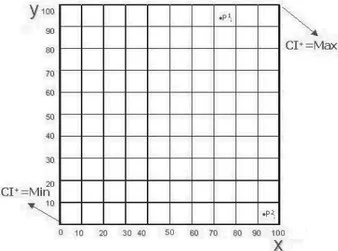
Unit i is represented by point Phi(x ,ih y ) in the positive evaluations zone refer-hi
ring to item h, belonging to the square with side size 100 situated in the first quadrant (positive evaluations area). The same unit i is also represented by point
Qhi(xi*h, y ) in the negative evaluations zone, belonging to the square with side *hi
size 100 situated in the third quadrant (negative evaluations area). The position of the single units inside the two areas provides an immediate view of the positive (negative) level of the opinion obtained. As it is highlighted immediately in Figure 1, the position of point Phi( h
i
x , h
i
y ) on the upper right apex corresponds to a unit i that obtained all “Definitely YES” evaluations for item h, and therefore obtained
Figure 1 – Position of points Phi in the positive evaluations semi-plane.
Likewise, the position of point Phi( h i
x , h
i
y ) at the origin of the axes will
corre-spond to unit i , which obtained no positive responses (no 1 or 2 responses but only 3 and 4) and that therefore obtained the minimum positive opinion. For any other situation, to establish whether unit 1 (represented by point 1
i
P ), which
ob-tained between 70% and 80% of positive opinions practically all “Definitely YES”, is associated with a more positive opinion than unit 2 (represented by point 2
i
P ) , which instead obtained more than 90% of positive opinions, though
practically all “More YES than NO), depends on the value opinion of the “inves-tigator/decision maker”, namely, on the degree of importance they want to assign to the quota of very positive opinions. Naturally, entirely analogous considera-tions are applicable to points Qhi(xi*h, y ) of the semi-plane referring to the i*h
negative evaluations. The index h
i
CI + is constructed on the basis of these considerations, with
refer-ence to the positive evaluations quadrant, is defined by:
100( )/ Max( )( ) 0 1 Max( ) 100(1 ) h h h h h i i i i i h i CI x ky CI CI k CI k + + + + = + ≤ ≤ = +
k represents the parameter selected by the “investigator” and expresses the level
of importance that they decide to assign to “very positive” opinions.
The process is likewise repeated for the negative quadrant by defining the fol-lowing index: * * 100( )/ Max( ) 0 1 Max( ) 100(1 ) h h h h i i i i h i CI x ky CI k CI k − − − = − + ≤ ≤ = − +
The index below is then established: h h h i i i CI =CI + +CI − with 100− ≤CIih ≤100
It can be seen immediately that selecting k=0, is equivalent to reducing the four-degree scale to a dichotomised one and therefore, choosing not to assign any weight to the responses “Definitely YES” and “Definitely NO”. In other words, the index becomes independent on the number of the responses assigned to the two extreme degrees (only very positive and very negative responses).
Example: The scenario involves two university courses. The first received 90% of positive opinions responding to the question about overall satisfaction, but these were all “More YES than NO”, while 10% of the negative opinions were all “Definitely NO”. The second received 70% of positive opinions, but these were all “Definitely YES”, while 30% of the negative opinions were all concentrated in the “More NO than YES” response. Selecting k=0, with P1(90,0), P2(70,100), Q1(10,100) and Q2(30,0) produces the following results:
CI+1=903 and CI+2=70 CI-1=-10 and CI-2=-30 and therefore: CI1=80 and CI2=40. Hence, course 2 would correspond to a value for the overall degree of satisfaction indicator equal to 50% of the value assigned to course 1.
Whereas by selecting k=1, the following results would be obtained:
CI+1=100(90/200)=45, CI+2=100(170/200)=85,
CI-1=-100(110/200)=-55, CI-2=-100(30/200)=-15 so that we would have: CI1=-10 and CI2=70.
It is evident that both results appear fairly unrealistic. Intermediate values of k lead, however, to more feasible evaluations. If we select, for example, k=0.5 with reference to the quadrant of positive evaluations (index CI+), it corresponds to assuming a global level of satisfaction of a first lesson, for which 100% of the participants replied “More YES than NO”, is equivalent to the result of a second lesson where only 50% of the participants replied “Definitely YES”, while the remaining 50% gave a negative reply. Obviously, the value of index CI in the two lessons will differ according to how the responses of the remaining 50% of the second group are distributed between the two negative modes.
With k =0.5, the result referring to the previous example, would be: CI+1=60,
CI+2=80, CI-1=-40, CI-2=-20 and, therefore, CI1=20 and CI2=60. In such a case, the second group corresponds more realistically to a higher overall level of satis-faction but, by contrast with the situation found with k=1, the first group also has a positive index, as it appears to be more consistent. The graph in figure 2 shows how the corresponding positions of two units vary as the choice of k changes.
Figure 2 – CI values for the global level of satisfaction of the two lessons as k varies.
3. THE DISTRIBUTIONS FOR DIFFERENT VALUES OF THE CI INDICES AND THEIR PROPERTIES 3.1. Four level scale
The distributional properties of the CI indices family were studied by adopting the following phases:
Phase 1: Construction of the universe of response models of N respondents. Starting from N=10, all the possible distributions of the responses submitted by the respondents (10, 0, 0, 0; 0, 10, 0, 0; ....), have been constructed and 286 separate response models have been obtained.
The same procedure was repeated for values of N up to 105 after setting gaps corresponding to 5.
Table 1 shows the number of response models for each of the values of N considered.
Phase 2: CI index calculation.
The CI values of the related response models were calculated for each N value, assigning values to parameter k, respectively, at 0; 0,1; 0,2; 0,3; 0,4; .... 0,9; 1, so that the effective distributions of the index are.
TABLE 1
Number of response models indicated separately for given values of N Number of respondents Number of response models Number of respondents Number of response models 10 286 60 39,711 15 816 65 50,116 20 1,771 70 62,196 25 3,276 75 76,076 30 5,456 80 91,881 35 8,436 85 109,736 40 12,341 90 129,760 45 17,296 95 152,096 50 23,426 100 176,851 55 30,856 105 204,156
Phase 3: Calculation of parameters for the CI indices distributions, for given N and k values.
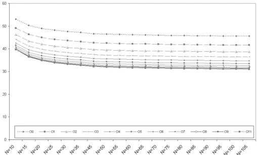
Figure 3 – Mean square error σ values for CI index distributions as N and k vary.
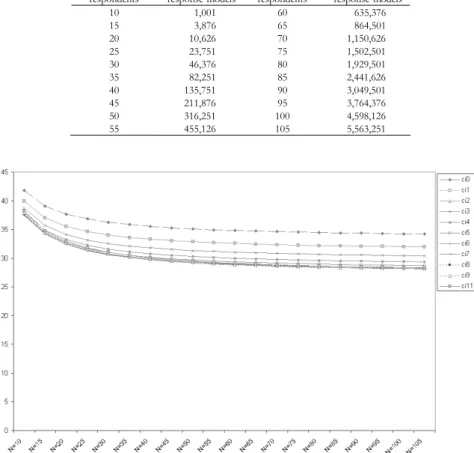
The results show that all the effective distributions are symmetric as N and k vary, with the mean, mode and median equal to 0. The mean square error σ as-sumes values lying between 53 and 31 and has a decreasing trend as k increases, whereas when N increases the trend always decreases but with variation rates tending towards zero. The graph in Figure 3 shows the trend of σ for the differ-ent distributions analysed.
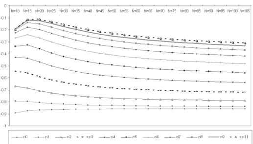
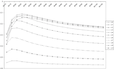
Each distribution has a finite and negative kurtosis index κ. As is well known, a distribution is normal if the kurtosis is equal to zero and therefore negative values indicate a leptokurtic type distribution. The trend of κ when k and N varying is more irregular compared to the trend of σ, but tends to stabilise for N values higher than 50 (Figure 4).
Figure 5 shows the frequency distributions observed and the corresponding expected theoretical distributions in the case of normality of index CI for 4 values of N and for 5 of k. As it can be seen, the deviations compared to the normal dis-tribution are somewhat limited, apart from the case where k=0. The frequency of values around the mean value is found to be lower than the normal distribution for values where k≤0.5. And as was to be expected, the match becomes distinctly better especially for k>0.5 as N increases.
Figure 4 – Kurtosis index κ values for CI index distributions as N and k vary.
Figure 5 – CI index distributions vs normal distributions.
The possibility of approximating CI distribution with a normal one offers in-teresting developments in an inferential framework.
In fact, once the level of significance has been established, it is possible to ver-ify the null hypothesis that the evaluation obtained from unit i with reference to the aspect identified by item h is not significantly different from the mean. As will be remembered, if the CI mean is 0, there is a substantial balance between posi-tive and negaposi-tive opinions. It is therefore possible to determine the critical value
of the positive or negative CI index that results in a rejection of the null hypothe-sis: it follows that the opinion expressed by the N evaluators can be considered significantly positive (negative).
With reference to the different aspects investigated, the evaluations obtained by unit i can be compared by using “means” for dependent samples.
Finally, a comparison between “means” can be made for independent samples if the aim is to compare the assigned evaluations for a given item to two or more units (regardless of the number Ni of evaluators of the i-th unit, provided they are
not under 50).
As an example, tables 2-4 show the values of the 90-th, the 95-th and the 99-th percentile of the CI index both with reference to the effective distribution (ob-served values) and the normal distribution (theoretical values) of parameters µ=0 and σ=σobserved in relation to the values of N equal to 30, 60, 70, 80, 105 and for the eleven values of k.
TABLE 2
Values of 90-th percentile of CI (observed values obs, theoretical values T and relative differeces ∆)
k N 0.0 0.1 0.2 0.3 0.4 0.5 0.6 0.7 0.8 0.9 1.0 30 obs 66.67 59.09 54.38 50.96 47.99 45.93 44.79 43.93 43.30 43.23 43.09 T 61.02 55.86 52.00 49.13 47.01 45.46 44.34 43.57 43.05 42.72 42.54 ∆ 0.09 0.06 0.05 0.04 0.02 0.01 0.01 0.01 0.01 0.01 0.01 50 obs 64.00 57.65 53.23 49.69 47.05 45.11 43.80 42.74 42.22 41.71 41.53 T 59.56 54.44 50.59 47.71 45.57 44.00 42.86 42.06 41.51 41.15 40.95 ∆ 0.07 0.06 0.05 0.04 0.03 0.03 0.02 0.02 0.02 0.01 0.01 70 obs 62.86 57.01 52.67 49.21 46.60 44.69 43.31 42.32 41.62 41.18 40.93 T 58.93 53.83 50.00 47.12 44.98 43.40 42.25 41.44 40.88 40.51 40.30 ∆ 0.07 0.06 0.05 0.04 0.04 0.03 0.03 0.02 0.02 0.02 0.02 90 obs 62.22 56.68 52.34 48.96 46.33 44.42 43.04 42.08 41.36 40.92 40.65 T 58.57 53.49 49.67 46.80 44.66 43.07 41.92 41.10 40.54 40.17 39.95 ∆ 0.06 0.06 0.05 0.05 0.04 0.03 0.03 0.02 0.02 0.02 0.02 105 obs 61.90 56.49 52.18 48.81 46.22 44.30 42.91 41.95 41.27 40.78 40.51 T 58.39 53.32 49.51 46.64 44.50 42.91 41.76 40.94 40.37 40.00 39.78 ∆ 0.06 0.06 0.05 0.05 0.04 0.03 0.03 0.02 0.02 0.02 0.02 TABLE 3
Values of 95-th percentile of CI (observed values obs, theoretical values T and relative differeces ∆) K N 0.0 0.1 0.2 0.3 0.4 0.5 0.6 0.7 0.8 0.9 1.0 30 obs 80.00 70.71 65.43 61.54 59.26 57.78 56.67 55.88 55.56 55.26 55.00 T 78.32 71.69 66.74 63.06 60.33 58.34 56.92 55.92 55.25 54.83 54.60 ∆ 0.02 -0.01 -0.02 -0.02 -0.02 -0.01 0.00 0.00 0.01 0.01 0.01 50 obs 76.00 69.13 63.99 60.18 57.59 55.83 54.61 53.82 53.33 52.96 52.77 T 76.45 69.87 64.93 61.24 58.49 56.47 55.01 53.98 53.27 52.82 52.56 ∆ -0.01 -0.01 -0.01 -0.02 -0.02 -0.01 -0.01 0.00 0.00 0.00 0.00 70 obs 74.29 68.40 63.33 59.56 56.95 55.09 53.90 52.99 52.41 52.09 51.91 T 75.63 69.09 64.17 60.48 57.73 55.70 54.23 53.18 52.46 52.00 51.72 ∆ -0.02 -0.01 -0.01 -0.02 -0.01 -0.01 -0.01 0.00 0.00 0.00 0.00 90 obs 75.56 67.99 62.96 59.25 56.62 54.76 53.47 52.60 52.02 51.65 51.46 T 75.18 68.66 63.75 60.07 57.32 55.29 53.81 52.75 52.03 51.55 51.27 ∆ 0.01 -0.01 -0.01 -0.01 -0.01 -0.01 -0.01 0.00 0.00 0.00 0.00 105 obs 75.24 67.78 62.79 59.05 56.43 54.60 53.29 52.41 51.82 51.42 51.25 T 74.95 68.44 63.54 59.86 57.11 55.08 53.60 52.54 51.81 51.34 51.05 ∆ 0.00 -0.01 -0.01 -0.01 -0.01 -0.01 -0.01 0.00 0.00 0.00 0.00
105 obs 90.48 82.29 77.59 74.77 72.92 71.67 70.81 70.29 69.92 69.76 69.63
T 106.00 96.80 89.87 84.66 80.78 77.90 75.81 74.31 73.28 72.61 72.20
∆ -0.15 -0.15 -0.14 -0.12 -0.10 -0.08 -0.07 -0.05 -0.05 -0.04 -0.04 In the case, for instance, of k=0.6 being chosen with the number N=70 evaluators, table 2 indicates that an index above or equal to 43.31 has a probabil-ity of occurring not over 10%, and the probabilprobabil-ity falls below 5% if the index is greater than 53.90 (table 3). If instead, reference is made to the normal distribu-tion, the critical values are 42.25 and 54.22, respectively. In the first case, the normal distribution is less conservative, in other words, it means rejecting the null hypothesis at a significance level lower than the pre-established level, and the op-posite is true in the second case.
3.2. Five level scale
As it is well known, in the cases where a scale with five degrees is adopted the central element indicates a neutral position of indifference and therefore neither a positive or negative opinion.
The expression of the CI index in this situation does not entail substantial changes. In fact, the unit i, as a consequence of the scores assigned to item h by the Nhi “evaluators”, will now correspond to the distribution Nhi(1), Nhi(2), Nhi(3),
Nhi(4), Nhi(5) of the frequencies associated with the five degrees of the scale, where Nhi(3) indicates the frequency of the “neutral” responses and
5 1 ( ) h h i i j N N j = =
∑
. We will obtain: xhi represents the % of the positive opinions for item h expressed by the
Nhi evaluators, where:
( (1) (2)) 100/
h h h h
i i i i
x = N +N ∗ N
yhi represents the % of the very positive opinions for item h calculated over the total of the positive opinions expressed by the Nhi evaluators, where:
(1) * 100/( (1) (2))
h h h h
i i i i
y =N N +N
*h ( h(4) h(5)) 100/ h
i i i i
x = N +N ∗ N
y represents the % of the very negative evaluations over the total of the *hi
negative evaluations:
*h h(5) * 100/( h(4) h(5))
i i i i
y =N N +N
Naturally, in this case, the equality *h
i
x =100 - h
i
x is no longer valid and the
number of possible response models associated with the number of opinions N increases significantly.
As for the even case we have calculated the number of response models gener-ated (Table 6), the distribution of the CI index for different values of N and k (Figures 5 and 6), the values of the 90-th percentile of CI index (Table 7), the val-ues of the 95-th percentile of CI index (Table 8), and the valval-ues of the 99-th per-centile of CI index (Table 9).
TABLE 6
Number of response models indicated separately for given values of N Number of
espondents esponse odels Number of Number of espondents esponse odels Number of
10 1,001 60 635,376 15 3,876 65 864,501 20 10,626 70 1,150,626 25 23,751 75 1,502,501 30 46,376 80 1,929,501 35 82,251 85 2,441,626 40 135,751 90 3,049,501 45 211,876 95 3,764,376 50 316,251 100 4,598,126 55 455,126 105 5,563,251
Figure 5 – Mean square error σ values for CI index distributions as N and k vary.
Figure 6 – Kurtosis index κ values for CI index distributions as N and k vary.
TABLE 7
Values of 90-th percentile of CI (observed values obs, theoretical values T and relative differeces ∆) K N 0.0 0.1 0.2 0.3 0.4 0.5 0.6 0.7 0.8 0.9 1.0 30 obs 53.33 48.29 44.96 42.56 40.98 40.00 39.58 39.37 39.51 39.68 40.00 T 50.55 46.48 43.64 41.73 40.49 39.75 39.36 39.24 39.29 39.48 39.75 ∆ 0.05 0.04 0.03 0.02 0.01 0.01 0.01 0.00 0.01 0.01 0.01 50 obs 52.00 46.78 43.53 41.20 39.58 38.56 38.02 37.75 37.78 37.89 38.15 T 49.08 45.00 42.13 40.16 38.86 38.05 37.61 37.42 37.43 37.56 37.79 ∆ 0.06 0.04 0.03 0.03 0.02 0.01 0.01 0.01 0.01 0.01 0.01 70 obs 50.00 46.14 42.93 40.62 39.00 37.98 37.39 37.11 37.06 37.18 37.41 T 48.44 44.37 41.49 39.51 38.18 37.35 36.88 36.67 36.65 36.77 36.98 ∆ 0.03 0.04 0.03 0.03 0.02 0.02 0.01 0.01 0.01 0.01 0.01 90 obs 50.00 45.79 42.59 40.29 38.68 37.65 37.05 36.76 36.70 36.80 37.01 T 48.08 44.02 41.14 39.15 37.82 36.97 36.49 36.27 36.23 36.34 36.53 ∆ 0.04 0.04 0.04 0.03 0.02 0.02 0.02 0.01 0.01 0.01 0.01 105 obs 49.52 45.61 42.44 40.13 38.53 37.49 36.89 36.59 36.51 36.61 36.82 T 47.90 43.84 40.97 38.98 37.64 36.79 36.30 36.07 36.03 36.13 36.32 ∆ 0.03 0.04 0.04 0.03 0.02 0.02 0.02 0.01 0.01 0.01 0.01 TABLE 8
Values of 95-th percentile of CI (observed values obs, theoretical values T and relative differeces ∆) K N 0.0 0.1 0.2 0.3 0.4 0.5 0.6 0.7 0.8 0.9 1.0 30 obs 66.67 59.85 55.96 53.46 51.95 51.11 50.78 50.75 50.93 51.03 51.58 T 64.87 59.65 56.02 53.56 51.97 51.02 50.52 50.36 50.43 50.67 51.02 ∆ 0.03 0.00 0.00 0.00 0.00 0.00 0.01 0.01 0.01 0.01 0.01 50 obs 64.00 57.95 54.10 51.47 49.82 48.84 48.35 48.22 48.22 48.42 48.74 T 62.99 57.76 54.07 51.54 49.87 48.84 48.27 48.03 48.04 48.21 48.51 ∆ 0.02 0.00 0.00 0.00 0.00 0.00 0.00 0.00 0.00 0.00 0.00 70 obs 62.86 57.14 53.32 50.67 48.98 47.94 47.38 47.17 47.19 47.37 47.64 T 62.17 56.95 53.25 50.70 49.01 47.94 47.34 47.07 47.04 47.19 47.46 ∆ 0.01 0.00 0.00 0.00 0.00 0.00 0.00 0.00 0.00 0.00 0.00 90 obs 61.90 56.49 52.69 50.04 48.30 47.25 46.66 46.40 46.38 46.53 46.79 T 61.71 56.50 52.80 50.25 48.54 47.46 46.83 46.55 46.51 46.64 46.89 ∆ 0.00 0.00 0.00 0.00 0.00 0.00 0.00 0.00 0.00 0.00 0.00 105 obs 61.90 56.49 52.69 50.04 48.30 47.25 46.66 46.40 46.38 46.53 46.79 T 61.48 56.27 52.58 50.02 48.31 47.22 46.59 46.29 46.24 46.37 46.61 ∆ 0.01 0.00 0.00 0.00 0.00 0.00 0.00 0.00 0.00 0.00 0.00
TABLE 9
Values of 99-th percentile of CI (observed values obs, theoretical values T and relative differeces ∆) K N 0.0 0.1 0.2 0.3 0.4 0.5 0.6 0.7 0.8 0.9 1.0 30 obs 83.33 77.62 74.39 72.75 71.77 71.29 71.02 71.01 71.24 71.54 71.67 T 91.75 84.37 79.23 75.75 73.50 72.15 71.45 71.22 71.33 71.66 72.16 ∆ -0.09 -0.08 -0.06 -0.04 -0.02 -0.01 -0.01 0.00 0.00 0.00 -0.01 50 obs 82.00 74.91 71.09 69.01 67.86 67.26 66.99 67.00 67.09 67.37 67.63 T 89.09 81.68 76.47 72.90 70.54 69.07 68.27 67.93 67.94 68.19 68.60 ∆ -0.08 -0.08 -0.07 -0.05 -0.04 -0.03 -0.02 -0.01 -0.01 -0.01 -0.01 70 obs 80.00 73.81 69.77 67.47 66.21 65.54 65.21 65.17 65.26 65.46 65.75 T 87.93 80.54 75.32 71.71 69.31 67.80 66.95 66.57 66.53 66.74 67.12 ∆ -0.09 -0.08 -0.07 -0.06 -0.04 -0.03 -0.03 -0.02 -0.02 -0.02 -0.02 90 obs 80.00 73.20 69.08 66.69 65.35 64.62 64.28 64.19 64.28 64.48 64.75 T 87.27 79.90 74.68 71.07 68.65 67.12 66.24 65.83 65.77 65.96 66.32 ∆ -0.08 -0.08 -0.07 -0.06 -0.05 -0.04 -0.03 -0.02 -0.02 -0.02 -0.02 105 obs 79.05 72.90 68.75 66.31 64.93 64.18 63.82 63.72 63.80 63.99 64.27 T 86.95 79.59 74.37 70.75 68.32 66.78 65.89 65.47 65.40 65.58 65.92 ∆ -0.09 -0.08 -0.08 -0.06 -0.05 -0.04 -0.03 -0.03 -0.02 -0.02 -0.03 4. FINAL REMARKS
The use of the CI index requires some caution. First of all it is important takes into account that this index is influenced by a “dimension effect” since it is based on percentages, so that in order to compare several units correctly on the basis of the values they have assumed, it is important for the number of respondents to be very similar or, at least, that there are no units with a very low number of respondents.
Secondly, if the computation of CI index is aimed to compare the evaluations on different dimensions of the service by the same group of respondents then the hypothesis of “unconditional behaviour” of the respondents doesn’t highlight any relevance.
This hypothesis could be verified to compare judgements on same service (dis-cipline, etc.) used by two o three groups of customers. However, the addiction of an adequate pool of items inside the questionnaire could be required by the set-ting free of “unconditional behaviour” hypothesis.
Dipartimento di Economia Politica MARISA CIVARDI
Università di Milano-Bicocca
Diparimento di Scienze Economiche Matematiche e Statistiche CORRADO CROCETTA
Università di Foggia
Dipartimento di Economia Politica EMMA ZAVARRONE
Università di Milano-Bicocca
REFERENCES
M. CIVARDI, E. ZAVARRONE (2003), How Difficulties, Didactic Supports and Teaching Quality in
Dis-ciplines Can Be Perceveid Through the Structural Approach, in “ISI 54th Session 2003 Pro-ceedings”, August.
zioni positive e le ultime due (o le prime due) a valutazioni negative. Gli indici, calcolati par-tendo dalla distribuzione osservata delle risposte, sono normalizzati e assumono valori com-presi tra –100 (quando tutte le risposte sono concentrate sul grado associato alla massima negatività) e +100 (quando tutte le risposte sono concentrate sul grado associato alla massi-ma positività, e cioè nel caso di assoluta eccellenza). Essi sono ottenuti come sommassi-ma alge-brica di due indici, di cui il primo esprime il punteggio ottenuto sul versante delle valutazioni positive ed il secondo su quello delle valutazioni negative. Il loro calcolo richiede la scelta da parte del ricercatore del valore da attribuire a un parametro k (0 ≤ k ≤ 1) che esprime il livel-lo di importanza che egli decide di attribuire alle opinioni “massimamente positive” e “mas-simamente negative”. La costruzione dell’universo dei modelli di risposta di N rispondenti (con 10≤ N ≤ 105 ed il calcolo, per ciascuno di essi, dei valori dell’indice CI corrispondenti a 11 valori del parametro k (0, 0.1, 0.2,..., 0.9, 1) ha consentito di studiare le proprietà delle distribuzioni effettive dell’indice. I risultati mostrano che tutte le distribuzioni effettive, al variare di k e di N, sono simmetriche con media, moda e mediana uguale a 0 e scarto qua-dratico medio σ che da un massimo di 53 (N=10 e k=0) scende, stabilizzandosi intorno a 31 al crescere di N e di k. La possibilità di approssimare la distribuzione di CI con una normale offre interessanti sviluppi in ambito inferenziale.
SUMMARY
Summary indicators of opinions expressed by the users of given service
In this paper we study the properties of a family of index, called CI. These indices have been proposed by Civardi, Zavarrone (2003) in order to evaluate the teaching quality in university disciplines. The most frequently used scales offer four or five points and the first two (or the last two) points on both scales are associated with negative evaluations and the last two (or the first two) are associated with symmetric positive evaluations.
The empirical distribution of responses represents the starting point to compute the CI indices. Each index assumes values lying between –100 (in the case of maximum negative evaluation) to +100 (in the case of an evaluation of absolute excellence) and is obtained as the algebraic sum of two indices. The first expresses the score obtained in the semi-plane of positive evaluations while the second represents the score obtained in the semi-plane of negative evaluations.
The CI index is characterized by the choice of the parameter of importance level k (0≤k≤1) on the degree of importance the “investigator/decision maker” wants to assign to the quota of very positive opinions and of the very negative ones.
The construction of the universe of response models of N respondents (with 10≤N≤105) and, for each distribution, of the eleven CI indices (k=0, 0.1, ..., 0.9, 1)) allow to study the properties of effective distributions of the indices. The results highlight that all effective distributions, varying N and k, are symmetric with mean, mode and median equal to zero. The square mean error assumes values from 53 (when N=10 and k=0) to 31. The possibility of approximating CI distribution with a normal one offers interesting developments in an inferential framework.