A COUNT MODEL BASED ON MITTAG-LEFFLER INTERARRIVAL TIMES
K.K. Jose, B. Abraham
1. INTRODUCTION
The common regression model for the number of events in a given interval of time (count data) used by most researchers is the Poisson model. The widespread popularity of the Poisson model for count data arises from its simple derivation as the number of arrivals in a given time period assuming exponentially distrib-uted interarrival times. But of the many other count models that have been de-veloped over the years, see (Wimmer and Altmann, 1999), very few share this straightforward connection between a count model and its timing model equiva-lent.
From the relationship between a count model and its timing process, a re-searcher can develop a model using one form (timing or counting) but apply it using the other. For example, marketing managers frequently collect interarrival time data and make predictions of the number of arrivals (purchases) that a par-ticular customer is likely to make over the next year.
The Poisson count model is valid only in the case where the data of interest support the restrictive assumption of equi-dispersion, that is the conditional vari-ance equals the conditional mean, but typically the conditional varivari-ance exceeds the conditional mean (over-dispersion). There are also cases where the condi-tional mean exceeds the condicondi-tional variance (under-dispersion). In either case, the estimation based on Poisson model is inefficient and leads to biased inference see (Winkelmann, 1995b). Thus the Poisson model becomes inadequate in most of the econometric applications.
We assume that the waiting times between the events are independent but not exponential (which would lead to the Poisson distribution for counts). Instead they follow some other distribution with a nonconstant hazard function. If the hazard function is a decreasing function of time, the distribution displays negative duration dependence. If the hazard function is an increasing function of time, the distribution displays positive duration dependence. In both cases, the conditional probability of a current occurrence depends on the time since the last occurrence rather than on the number of previous events. Events are dependent in the sense
that the occurrence of at least one event (in contrast to none) up to time t influ-ences the probability of a further occurrence in tt. There is a link between duration dependence and dispersion. It is shown that negative duration depend-ence (asymptotically) causes over-dispersion and positive duration dependdepend-ence causes under-dispersion.
The Poisson process can be taken as a sequence of independently and identi-cally exponentially distributed waiting times see (Cox, 1972). To derive a general-ized model we replace the exponential distribution with a less restrictive non negative distribution. Possible candidates are the Weibull see (McShane et al., 2008), the gamma (including generalized gamma) see (Winkelmannn, 1995a), and the log normal distributions. Both Weibull and gamma nest the exponential dis-tribution and both allow for a monotone hazard rate function that is duration de-pendent.
In this paper we develop a new generalized model by replacing the exponential distribution by Mittag-Leffler distribution which is a generalization of exponential distribution. A corresponding count model is formulated. Advantages of this generalized count model are the following. First our count model is based upon an assumed Mittag-Leffler inter-arrival process which nests the exponential as a well known special case. Second, we demonstrate that the Mittag-leffler count model, via the shape parameter can capture over-dispersed as well as equi-dispersed data. Third, the Mittag-Leffler inter arrival time story is richer than the exponential story, because it allows for nonconstant hazard rates (duration de-pendence). Fourth, we implement the model entirely in standard software. This is accomplished by deriving our model using a polynomial expansion (which can be expressed in closed form) see (Bradlow et al., 2002), (Everson et al., 2002), (Miller
et al., 2006) for similar polynomial expansion solutions for negative binomial, beta
binomial and binary logit models respectively.
The remainder of this article is as follows. In section 2, a description about Mittag-Leffler distribution is given. Section 3 contains the derivation of the Mit-tag-Leffler count model, focusing on the polynomial expansion that leads to the closed form benefits. In section 4 we derive the properties of the new Mittag-Leffler count model and present the results of a simulation study pertaining to the new model. Application of this new counting model to a real data is explained in section 5.The mathematical derivations are given in the Appendix.
2. MITTAG-LEFFLER DISTRIBUTION The function ( ) = =0 (1 ) k k z E z ak
was first introduced by Mittag-Leffler in 1903. It was subsequently investigated by Wiman, Pollard, Humbert, Aggarwal and Feller. Many properties of the function follow from Mittag-Leffler integral rep-resentation. During the last two decades this function has come into prominence after about nine decades of its discovery by a Swedish Mathematician G.M.
Mittag-Leffler, due to the vast potential of its applications in solving the problems of physical, biological, engineering and earth sciences etc. The Mittag-Leffler function arises naturally as the solution of fractional order integral equations or fractional order differential equations, and especially in the investigations of the fractional generalization of the kinetic equation, random walks, Levy flights, super-diffusive transport and in the study of complex systems. It may be verified that
1 1 ( ) 2 t t e E z C dt i t z
where the path of integration C is a loop which starts and ends at and en-circles the circular disc
1
| |t z. It may be noted that (Pillai, 1990) proved that
( ) = 1 ( ),0 < 1
F x E x are distribution functions, having the Laplace
transform ( ) = (1t t) ,1 > 0t which is completely monotone for 0 < . 1
He called F x( ),0 < , a Mittag-Leffler distribution. The Mittag-Leffler dis-1 tribution is a generalization of the exponential distribution, since for = 1 , we get exponential distribution. Pillai has shown that F x( ) is geometrically infi-nitely divisible (g.i.d.) and is in the domain of attraction of stable laws. The Mit-tag-Leffler distribution can be defined as follows.
A random variable X has the Mittag-Leffler distribution if its cumulative dis-tribution function [c.d.f.] has the form
1 =1 ( 1) ( ; ) = , > 0,0 < 1 (1 ) k k k x F x x k (1)
and the p.d.f. is given by,
1 1 =1 ( 1) ( ; ) = , > 0,0 < 1. (1 , ) k k k k x f x x k (2)
Recently Mittag-Leffler distributions have received the attention of mathemati-cians,statisticians and scientists in physical and chemical sciences. It can be used in reliability modeling as an alternative for exponential distribution see (Lin, 1998), (Jayakumar, 2003), (Jayakumar and Pillai, 1993), (Jose and Pillai, 1996) have done extensive studies on Mittag-Leffler distribution and its applications. (Jose et
al., 2010) extended this to develop a more generalized Mittag-Leffler model.
3. MITTAG-LEFFLER COUNT MODEL
We can describe a general framework utilized to derive the model that is based upon the relationship between interarrival times and their count model
equiva-lent. Let Y be the time from the measurement origin at which the n n event oc-th curs. Let X t denote the number of events that have occurred upto time t. The ( ) relationship between interarrival times and the number of events is
( ) n Y t X t n Hence 1 ( ) = [ ( ) = ] = [ ( ) ] [ ( ) 1] = [ ] [ ] n n n M t P X t n P X t n P X t n P Y t P Y t
If we let the c.d.f. of Y as ( )n F t , then n 1
( ) = [ ( ) = ]= ( ) ( )
n n n
M t P X t n F t F t . (3)
In the case where the measurement time origin (and thus counting process) co-incides with the occurrence of an event, ( )F t is simply the n-fold convolution of n the common interarrival time distribution which may or may not have a closed form solution. Now we assume that the interarrival times are independent and identically distributed according to Mittag-Leffler distribution. To obtain equation (3) we use a recursive relationship of the form
1 0 0 1 0 ( ) ( ) ( ) ( ) ( ) = ( ) ( ) t t n n n t n M t F t s f s ds F t s f s ds M t s f s ds (4)
Before proceeding to develop the general solution to the problem, we note that F t = 1 and 0( ) F t1( ) = ( )F t for every t. Therefore we have
0 0 1 =0 ( 1) ( ) = ( ) ( ) = 1 ( ) = (1 ) k k k t M t F t F t F t k
By equation (4) we can derive
1 0 0 1 =1 ( ) ( ) ( ) ( 1) = (1 ) t l l l M t M t s f s ds l t l Similarly, 2 2 =2 ( 1) 2 ( ) = (1 ) l l l l t M t l
Thus we obtain a general form for M t which is given in the following theo-n( ) rem.
Theorem. If the interarrival times are independently and identically distributed as
Mittag-Leffler distribution, then the count model probabilities are given by
( ) = ( 1) ( ) = [ ( ) = ]= , = 0,1, 2... (1 ) j n j n j n j t n M t P X t n n j (5) 4. PROPERTIES
1. The Mittag-Leffler count model generalizes the most commonly used model such as Poisson as special case. When = 1,
( ) = ( 1) ( ) ( ) = [ ( ) = ]= = (1 ) ! j n j n j n n j t t n t e M t P X t n j n
This is a Poisson process with unit rate.
2. Mean and variance of the Mittag-Leffler count model exist and are obtained as = [ ( )] = (1 ) t Mean E X t 2 2 [ ( )] = 2 (1 ) (1 2 ) (1 ) t t t V X t .
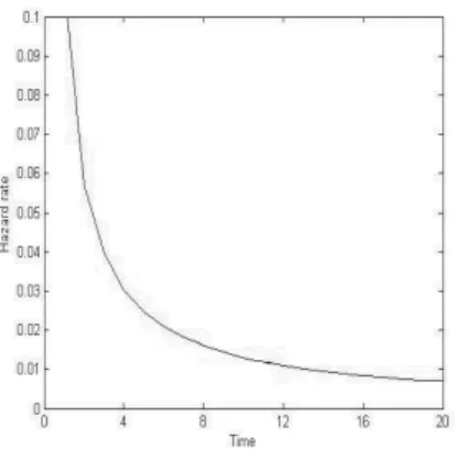
3. The hazard function is
1 1 =1 =0 ( 1) (1 ) ( ) ( ) = = . 1 ( ) ( 1) (1 ) k k k k k k k t k f t h t F t t k
Through extensive simulations, we have verified that the hazard function of the Mittag-Leffler distribution is a decreasing function of time (Figure 1 and 2
supports this intuitive fact), so that the distribution displays negative duration de-pendence which causes over-dispersion. The hazard function is a function of ,
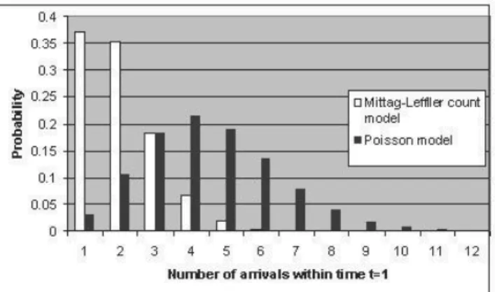
0 < . The model can handle over-dispersed as well as equi-dispersed data 1 when 0 < < 1 and = 1 respectively. Figure 3 displays the probability histo-gram for an overdispersed Mittag-Leffler count model and equi-dispersed Pois-son model.
Figure 1 – Hazard rate of Mittag-Leffler count Figure 2 – Hazard rate of Mittag-Leffler count
model (α = 0.2). model (α =0.9).
Figure 3 – Probability histogram of Mittag-Leffler count model (α=0.5) and Poisson model (λ=2).
4. If the inter arrival times of the data set are Mittag-Leffler distributed then, we have a corresponding counting model to use. The model (5) is derived from Mit-tag-Leffler timing model, the link between the timing model and its counting model equivalent is maintained. Hence in those cases where an analysis of the in-terarrrival times suggests that a more flexible timing model is needed, it can now
be incorporated via its count model equivalent. Furthermore, in those cases where one only has count data, but would like to make forecasts of the next arri-val time, this can be done given the timing and count model link that is now achieved.
5. The probability generating function of the Mittag-Leffler count model can be derived as =0 1/ ( ) = ( ( ) = ) = 1 [ (1 ) ] n n P s P X t n s F t s
6. If ( )X t is a Mittag-Leffler count process, then the autocorrelation coefficient
between ( )X t and (X t s is obtained as )
1/2 [ ( ), ( )] ( , ) = [ [ ( )]. [ ( )]] Cov X t X t s t t s V X t V X t s
where Cov[X(t),X(t+s)] = E[X(t) X(t+s)] – E[X(t)] E[X(t+s)] and 2 2 ( ) 2 [ ( ) ( )]= (1 ) (1 2 ) ( (1 ) ) ts t t E X t X t s .
7. Among MCMC methods Metropolis-Hastings algorithm is used to simulate the Mittag- leffler count model. The model is computationally feasible to work with and it is estimable without requiring a formal programming language or time con-suming simulation based methods.
TABLE 1
Table showing values of autocorrelation of the Mittag-Leffler count model for different values of the parameter at t = 1,2,3 and s = 1,2,3
t = 1 t = 2 t = 3 s = 1 s = 2 s = 3 s = 1 s = 2 s = 3 s = 1 s = 2 s = 3 0.1 0.6284 0.5963 0.5729 0.5894 0.5714 0.5555 0.5623 0.5515 0.5402 0.2 0.5519 0.4965 0.4579 0.4852 0.4553 0.4298 0.4411 0.4235 0.4058 0.3 0.5038 0.4299 0.3806 0.4159 0.3775 0.3460 0.3605 0.3384 0.3171 0.4 0.4748 0.3850 0.3276 0.3695 0.3244 0.2889 0.3060 0.2806 0.2571 0.5 0.4598 0.3551 0.2910 0.3393 0.2884 0.2497 0.2693 0.2413 0.2163 0.6 0.4552 0.3361 0.2659 0.3211 0.2646 0.2232 0.2456 0.2150 0.1888 0.7 0.4588 0.3254 0.2497 0.3127 0.2503 0.2062 0.2324 0.1989 0.1713 0.8 0.4688 0.3216 0.2409 0.3128 0.2439 0.1970 0.2285 0.1914 0.1621 0.9 0.4832 0.3240 0.2397 0.3204 0.2444 0.1948 0.2342 0.1921 0.1607 1 0.5000 0.3333 0.2500 0.3333 0.2500 0.2000 0.2500 0.2000 0.1667
TABLE 2
Table showing values of Mittag-Leffler count model probabilities for different values of the parameter
at t = 1,2,3 t = 1 t = 2 t = 3 M t1( ) M t2( ) M t3( ) M t1( ) M t2( ) M t3( ) M t1( ) M t2( ) M t3( ) 0.2 0.2533 0.1339 0.0679 0.2501 0.1412 0.0787 0.2471 0.1447 0.0836 0.3 0.2577 0.1398 0.0733 0.2502 0.1500 0.0874 0.2433 0.1537 0.0947 0.4 0.2642 0.1466 0.0766 0.2505 0.1596 0.0968 0.2378 0.1624 0.1063 0.5 0.2732 0.1544 0.0792 0.2518 0.1832 0.1191 0.2304 0.1709 0.1189 0.6 0.2852 0.1628 0.0807 0.2518 0.1832 0.1191 0.2207 0.1794 0.1329 0.7 0.3006 0.1713 0.0801 0.2534 0.1986 0.1326 0.2084 0.1881 0.1491 0.8 0.3197 0.1786 0.0768 0.2563 0.2176 0.1478 0.1929 0.1977 0.1686 0.9 0.3424 0.1834 0.0704 0.2615 0.2413 0.1642 0.1734 0.2090 0.1929 1 0.3679 0.1839 0.0613 0.2707 0.2707 0.1804 0.1494 0.2240 0.2240
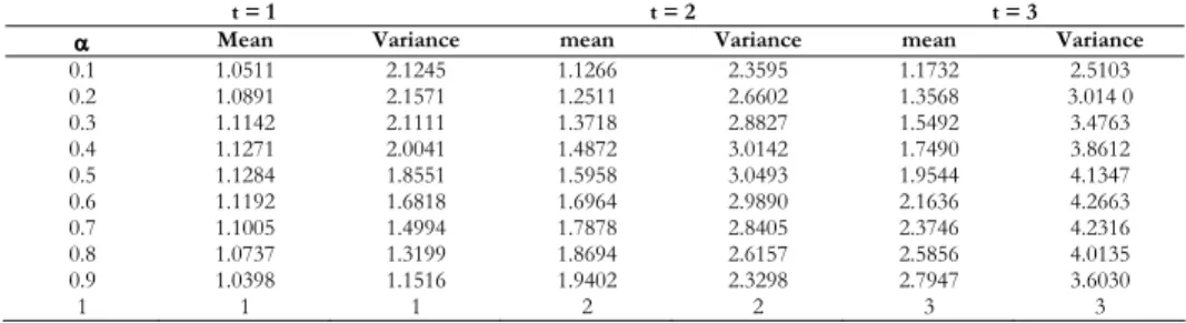
Table 1 gives the values of autocorrelation function for different values of , t and s. The auto correlation of the process increases as the parameter de-creases. Table 2 gives the probabilities of Mittag-Leffler count model for different values of the parameter at t = 1,2 and 3. By using Metropolis-Hastings algo-rithm we simulate the Mittag-Leffler count model and verified that for 0< 1 the conditional variance exceeds conditional expectation which represents the overdispersion, but for = 1 conditional mean equals conditional variance at t = 1, 2 and 3 which means the equidispersion. Thus Mittag-Leffler count model can be used to represent overdispersed as well as equidispersed real data. Table 3 supports this intuitive fact.
TABLE 3
Table showing values of mean and variance of the Mittag-Leffler count model probabilities for different values of the parameter at t = 1,2,3
t = 1 t = 2 t = 3
Mean Variance mean Variance mean Variance
0.1 1.0511 2.1245 1.1266 2.3595 1.1732 2.5103 0.2 1.0891 2.1571 1.2511 2.6602 1.3568 3.014 0 0.3 1.1142 2.1111 1.3718 2.8827 1.5492 3.4763 0.4 1.1271 2.0041 1.4872 3.0142 1.7490 3.8612 0.5 1.1284 1.8551 1.5958 3.0493 1.9544 4.1347 0.6 1.1192 1.6818 1.6964 2.9890 2.1636 4.2663 0.7 1.1005 1.4994 1.7878 2.8405 2.3746 4.2316 0.8 1.0737 1.3199 1.8694 2.6157 2.5856 4.0135 0.9 1.0398 1.1516 1.9402 2.3298 2.7947 3.6030 1 1 1 2 2 3 3
5. APPLICATION TO A REAL DATA SET
In this section we apply the model to a data on the time between customer ar-rivals for all customers arriving in a bank on a given day taken from the file Bank.arrivals.xlsx available in the website www.westminstercollege.edu. The inter arrivals times are clearly positively skewed. There is a long tail to the right of the peak and none to the left. All interarrival times are expressed in minutes and the total number of customers arriving in a bank on a randomly selected day is 275. In the data, values over 15 minutes are quite unlikely and there is usually very
lit-tle time between consecutive customer arrivals. Now and then, there is a fairly large gap between arrivals. Here the conditional mean is smaller than the condi-tional variance.(mean = 3.5174 and variance = 8.2988) Thus this dataset is overdispersed and hence we apply the Mittag-Leffler count model.
Figure 4 – The histogram of real data and the frequency curve of Mittag-Leffler distribution.
To test whether there is a significant difference between an observed inter arrival time distribution and the Mittag-Leffler distribution, we use Kolmogorov-Smirnov [K.S.] test for H : Mittag-Leffler distribution with parameter 0 = 0.95 is a good fit
for the given data. Here the calculated value of the K.S. test statistic is 0.098181 and the critical value corresponding to the significance level 0.01 is 0.098292, showing that the Mittag-Leffler assumption for interarrival times is valid.
To estimate the number of customers in a class we use the Mittag-Leffler count model. The Mittag-Leffler count model can be applied to the overdispersed data as well as equidispersed data in which case it coincides with the Poisson model. The figure 5 supports this fact clearly.
Figure 5 – Probability histogram of the predicted number of customers arriving in a bank according
CONCLUSIONS
In this article we have introduced a new count model based upon Mittag-Leffler inter arrival time process. More importantly, the model provided a size-able improvement over the more traditional Poisson process. One important ad-vantage of the new model is that it removed the artificial symmetry between overdispersion and equidispersion, a violation of the constant hazard assumption underlying the Poisson model. This new model can be treated as a generalization of the Poisson process. The new model has closed form nature and computation is possible using Matlab. This new model can be applied to real data sets where the assumption of equidispersion is violated.
ACKNOWLEDGEMENTS
The authors are grateful to the reviewers for the suggestions which helped in improv-ing the contents of the paper.
Department of Statistics KANICHUKATTU K. JOSE
St. Thomas College, Pala, Arunapuram Mahatma Gandhi University, Kerala, India
Department of Statistics BINDU ABRAHAM
Baselios Poulose II Catholicose College, Piravom Mahatma Gandhi University, Kerala, India
REFERENCES
BLAKE MCSHANE, M. ADRIAN, E.T. BRADLOW, and P.S. FADER (2008), Count models based on Weibull interarrival times, “Journal of Business and Economic Statistics”, 26, No. 3, 369-378.
E.T. BRADLOW, B.G.S. HARDIE, and P.S. FADER (2002), Bayesian Inference for the Negative Binomial Distribution via Polynomial Expansions, “Journal of Computational and Graphical Statis-tics”, 11, 189-201.
D.R. COX (1972), Regression Models and Life Tables, “Journal of the Royal Statistical Society”, Ser. B, 34,187-220.
P.J. EVERSON, and E.T. BRADLOW (2002), Bayesian Inference for the Beta binomial distribution via polynomial expansion, “Journal of Computational and Graphical Statistics”, 11, 202-207.
K.JAYAKUMAR, and R.N. PILLAI (1993), The first order Autoregressive Mittag-Leffler process, “Journal of Applied Probability”, 30, 462-466.
K. JAYAKUMAR (2003), On Mittag-Leffler process, “Mathematical and Computer Modelling”, 37, 1427-1434.
K.K. JOSE, and R.N. PILLAI (1996), Generalized Autoregressive Time series models in Mittag-Leffler variables, “Recent Advances in Statistics”, 96-103.
K.K. JOSE, P. UMA, V. SEETHALEKSHMI, and H.J. HAUBOLD (2010), Generalized Mittag-Leffler Proc-esses for Applications in Astrophysics and Time Series Modelling, “Astrophysics and Space Sci-ence Proceedings”, DOI: 10.1007/978-3-642-03325-4.
G.D. LIN (1998), On the Mittag-Leffler distributions, “Journal of Mathematical Anal. Appl”., 217, 701-706.
S.J. MILLER, E.T. BRADLOW, and K. DAYARATNA (2006), Closed form Bayesian inferences for the logit model via Polynomial expansions, “Quantitative Marketing and Economics”, 4, 173-206.
R.N. PILLAI (1990), On Mittag-Leffler and related distributions, “Ann. Inst. Statist. Math.”, 42. No. 1, 157-161.
G. WIMMER, and G. ALTMANN (1999), Thesaurus of Univariate Discrete Probability Distributions, Germany, “Stamm Verlag”.
R. WINKELMANN (1995a), Duration dependence and Dispersion in Count data models, “Journal of Business and Economic Statistics”, 13, 467-474.
R. WINKELMANN (1995b), Recent developments in Count data modeling theory and applications,
APPENDIX
Appendix 1: Derivation of Mittag-Leffler count model probabilities
1 0 0 1 1 0 =0 =1 1 1 0 =0 =1 1 =0 =1 ( ) = ( ) ( ) ( 1) ( ) ( 1) = (1 ) (1 ) ( 1) ( 1) = [ ( ) ] (1 ) (1 ) ( 1) ( 1) = (1 ) (1 ) t j j k k t j k j k t k j j k j k k j k M t M t s f s ds t s k s ds j k k s t s ds j k t j k
j(1(1jj) (1k)k) 1 =0 =1 ( 1) ( 1) = (1 ) j k k j j k t j k
By using a change of variables =m j and =l m k we obtain
1 ( ) 1 1 =1 =0 1 1 =1 =0 1 =1 ) ) ( 1) ( 1) ( ) (1 ( ) ) ( 1) = (1 ( 1) = (1 m l m m l m l l m l l l l m l l l t M t m l m t l l t l
2 0 1 1 1 1 0 =1 =1 1 1 =1 =1 , ( ) = ( ) ( ) ( 1) ( ) ( 1) = (1 ) (1 ) ( 1) ( 1) = (1 ) t j j k k t j k j k k j j k Similarly M t M t s f s ds j t s k s ds j k j t j k
By using a change of variables =m j and =l m k we obtain 2 2 =2 ( 1)( 1) ( ) = 2 (1 ) l l l l l t M t l
2 = 2 ( 1) 2 = (1 ) l l l l t l
1 0 1 1 0 = =1 1 = =1 ( ) = ( ) ( ) ( 1) ( ) ( 1) = (1 ) (1 ) ( 1) ( 1) = (1 ) t n n j n j k k t j n k j n k k j j n k M t M t s f s ds j t s n k s ds j k j t n j k
By using a change of variables =m j and =l m k we obtain
( 1) 1 = 1 ( 1) 1 ( ) = (1 ) l n l n l n l t n M t l
Appendix 2: The probability generating function of the Mittag-Leffer count model =0 ( ) =0 = =0 1/ =0 1/ ( ) = ( ( ) = ) ( 1) = (1 ) ( 1) = (1 ) (1 ) ( 1) [ (1 ) ] = (1 ) = 1 [ (1 ) ] n n j n j n n j n j j j j j j j P s P X t n s j t n s j t s j t s j F t s
, SUMMARYA count model based on Mittag-Leffler interarrival times
In this paper, a new generalized counting process with Mittag-Leffler inter-arrival time distribution is introduced. This new model is a generalization of the Poisson process. The computational intractability is overcome by deriving the Mittag-Leffler count model using polynomial expansion. The hazard function of this new model is a decreasing function of time, so that the distribution displays negative duration dependence. The model is applied to a data on interarrival times of customers in a bank counter. This new count model can be simulated by Markov Chain Monte-Carlo (MCMC) methods, using Metropolis-Hastings algorithm. Our new model has many nice features such as its closed form na-ture, computational simplicity, ability to nest Poisson, existence of moments and autocor-relation and can be used for both equi-dispersed and over-dispersed data.