Polytechnic University of Marche
Faculty of Engineering
A dissertation for the degree of Philosophiae Doctor
In Civil, Environmental, Building Engineering and Architecture
Monitoring and Self-diagnosis of Civil Engineering Structures:
Classical and Innovative Applications
PhD Dissertation of: Alessio Pierdicca
Supervisor Prof. Stefano Lenci
Curriculum Supervisor Prof. Stefano Lenci
XXIX Edition November 2016
iii
Abstract
Extreme events like explosions and earthquakes may have a deep impact on building safety. Seismic regions must live with these tragic events, so that continuous monitoring of structure health conditions is necessary in many cases.
Structural Health Monitoring (SHM) represents a powerful tool for the evaluation of dynamic behavior of monitored structures. Until a few years ago these techniques were widely employed especially in mechanical, aeronautical and aerospace engineering.
Nowadays, the reduction of equipment costs, the new generation of data acquisition systems, together with the continuous improvement of computational analysis have made it possible to apply SHM also to civil structures without strategic importance. SHM has moved from large infrastructures like bridges, dams and skyscrapers to historical heritage and residential buildings.
In this background, the present work tries to examine different aspects of SHM applications, especially referred to ordinary buildings.
Using Operational Modal Analysis (OMA) techniques, several civil structures have been monitored through a wired network sensor, in order to obtain the dynamic behavior in operating conditions. The relevant data collection provides a useful tool for calibrating the accuracy and sensitivity of similar SHM case studies.
Specific attention is focused in another important issue in civil and in mechanical engineering: detection of structural damages. Through a numerical approach, a new method for damage localization and quantification is proposed.
Besides the traditional wired acquisition system a Wireless Sensor Network (WSN) has been developed. The issues related to the usage of low-cost sensors and new generation data acquisition tools for non-destructive structural testing are discussed. Using the WSN an historical masonry building has been monitored, showing the positive results obtained following the Ambient Vibration Survey (AVS).
v
Sommario
Eventi estremi come esplosioni o terremoti possono avere un profondo impatto nella sicurezza degli edifici. Le zone sismiche devono convivere con questi tragici eventi, per questo monitorare in maniera continua le condizioni di salute di una struttura è necessario e auspicabile in molti casi.
Il monitoraggio strutturale (Structural Health Monitoring – SHM) rappresenta un potente strumento per la valutazione del comportamento dinamico della struttura monitorata. Fino a pochi anni fa queste tecniche erano impiegate prevalentemente in ambito meccanico, aeronautico e nell’ingegneria aerospaziale.
Al giorno d’oggi, la riduzione dei costi della strumentazione, sistemi di acquisizione dati di nuova generazione e l’incremento continuo dell’efficienta nelle analisi numeriche hanno reso possibile l’applicazione di queste tecniche anche a strutture civili ordinarie.
Le tecniche di monitoraggio strutturale vengono applicate non solo in grandi infrastrutture come ponti, dighe o grattacieli, ma anche in strutture storiche o edifici residenziali.
In questo contesto questa tesi tenta di esaminare differenti aspetti del monitoraggio strutturale, in particolar modo riferite a edifici ordinari.
Attraverso tecniche Output-Only (Operational Modal Analysis – OMA) sono state monitorate diverse strutture civili con reti di sensori cablate, al fine di ottenere il comportamento dinamico strutturale nelle reali condizioni opertive.
Particolare attenzione è stata focalizzata in un altra importante tematica dell’ingegneria strutturale: il danneggiamento strutturale. Attraverso un approccio numerico viene presentato un nuovo metodo per la localizzazione e quantificazione del danno a seguito di un evento sismico.
In alternativa alla classica rete cablata, è stato sviluppato un sistema di acquisizione con sensori wireless (Wireless Sensor Network – WSN). I principali risultati ottenuti con questa applicazione vengono riportati nella presente tesi, unitamente al design dei sensori low-cost. Con l’ausilio della sensoristica sviluppata è stato monitorato un edificio storico in muratura, mostrando i risultati positivi ottenuti a seguito della campagna di acquisizione di rumore ambientale (Ambient Vibration Survey -AVS).
vii
Contents
Chapter 1
Introduction ... 1
1.1 Why SHM for civil applications ... 2
1.2 Thesis outline ... 3
Chapter 2 Structural Health Monitoring: State of art ... 5
2.1 Introduction to SHM ... 5
2.2 SHM Classifications ... 6
2.3 SHM applications ... 7
2.4 SHM general methods ... 8
Chapter 3 Output-Only Modal Identification ... 11
3.1 Introducing OMA ... 11
3.2 Structural Dynamics Models ... 14
3.2.1 Equation of motion and structural dynamic properties ... 14
3.2.2 State space models... 15
3.3 Characterization of Output-Only techniques ... 17
3.3.1 OMA in frequency domain ... 17
3.3.2 OMA in time domain ... 19
3.4 Stochastic Subspace Identification ... 19
3.4.1 The Kalman filter ... 20
3.4.2 Covariance-Driven Stochastic Subspace Identification ... 22
3.5 Post-Processing of Modal Parameter Estimates ... 25
3.5.1 Analysis of mode shapes ... 25
3.5.2 Analysis of natural frequencies ... 27
3.5.3 Modal Assurance Criterion (MAC) ... 28
3.5.4 Stabilization Diagrams for Parametric OMA Methods ... 29
Chapter 4 The measurement process ... 31
4.1 Instrumentation ... 31
viii
4.1.2 Transducers ... 34
4.2 Signal Processing ... 36
4.2.1 Data Acquisition Software ... 37
Chapter 5 Damage Detection ... 41
5.1 Introduction ... 41
5.2 Definition of Damage Index ... 42
5.2.1 Damage Indices: Classification ... 43
5.2.2 Review of the most commonly used damage indices ... 44
5.3 Damage detection in a civil structure subjected to an earthquake ... 47
5.3.1 Research motivation ... 47
5.3.2 Description of the structure ... 49
5.3.3 FEM model calibration with linear and nonlinear analysis ... 52
5.3.4 SHM implementation and damage indices ... 58
5.3.5 Final remarks ... 64
Chapter 6 SHM Applications ... 65
6.1 Introduction ... 65
6.2 Dynamic Identification of a precast industrial building ... 66
6.2.1 Research motivations ... 66
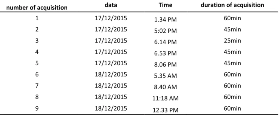
6.2.2 Ambient Vibration Survey ... 66
6.2.3 Updating of F.E. Model ... 70
6.3 One-year monitoring of a reinforced concrete school building ... 74
6.3.1 Research motivations ... 74
6.3.2 Ugo Foscolo school building ... 75
6.3.3 Long-term Ambient vibration tests ... 79
6.3.4 Estimation of the structural dynamic parameters ... 80
6.3.5 F.E. model updating ... 83
6.3.6 Final remarks ... 88
Chapter 7 Ambient Vibration Survey using Wireless Sensor Network ... 91
7.1 Introduction ... 91
7.2 Development of a Wireless Sensor Network ... 91
ix
7.2.2 Sensors calibration ... 96
7.3 AVS of a historical masonry building monitored with a WSN ... 99
7.3.1 Research motivation ... 99
7.3.2 Description of the structure ...100
7.3.3 Monitoring procedures and ambient vibration tests ...102
7.3.4 Dynamic Identification and F.E. modeling of the building ...105
7.3.5 Tuning of the NM ...108 7.3.7 Final remarks ...114 Chapter 8 Conclusions ... 115 References ... 117 Publications ... 125
xi
List of Figures
Figure 2.1 Simplified representation of stages involved in SHM process ... 8
Figure 3.1 Schematic illustration of LTI system ... 11
Figure 3.2 Schematic illustration of MDOF system ... 14
Figure 3.3 Complexity plot: (a) real/normal mode, (b) complex mode ... 26
Figure 3.4 Comparison between two sets of natural frequency ... 27
Figure 3.5 MAC: Comparison between two sets of natural frequency ... 28
Figure 3.6 Stabilization diagram ... 29
Figure 4.1 data acquisition system setup ... 31
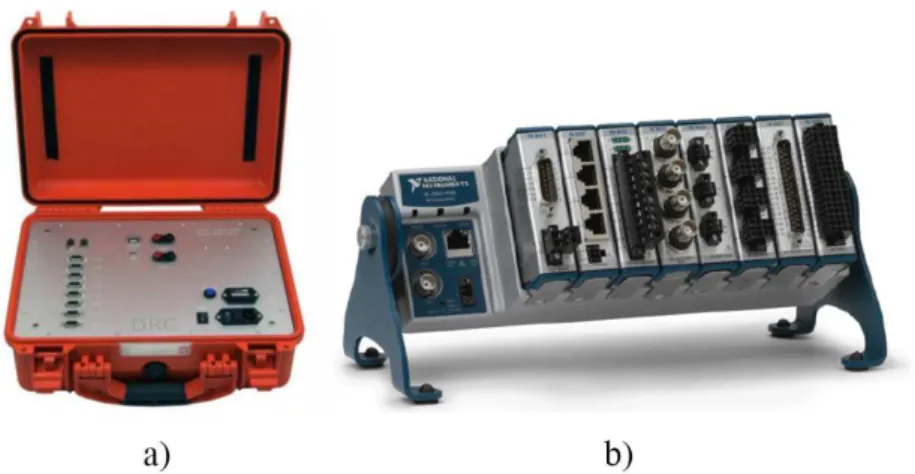
Figure 4.2 Dynamic data acquisition system DaTa500 by DRC – Diagnostic Research Company a),programmable hardware by National Instruments b) ... 32
Figure 4.3 Customizable solutions by National Instruments: (a) CDAQ 9132 data acquisition, (b) NI 9234 modules ... 33
Figure 4.4 Piezoelectric sensors: (a) KS48C and KB12VD accelerometers, (b) cross-section of KS48C sensor ... 35
Figure 4.5 Aliasing. True signal (3.5kHz), Aliased signal (0.5kHz) ... 36
Figure 4.6 The Measurement and Automation eXplorer ... 38
Figure 4.7 Front panel, channel management ... 38
Figure 5.1 SHM process: from acquisition to damage detection ... 41
Figure 5.2 Force-displacement relationship under monotonically increasing deformation 45 Figure 5.3 External view of the building. ... 50
Figure 5.4 (a) Plan view and (b) vertical sections of the building ... 51
Figure 5.5 Main dimensions of the cross-section elements: (a) columns, (b) (c) beams, (d) double T beams. ... 51
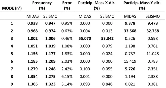
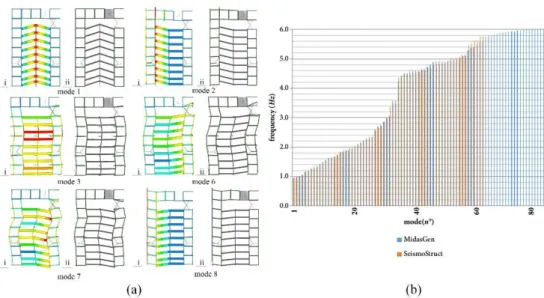
Figure 5.6 (a) Modal shapes with Seismostruct© (i) and MidasGen© (ii) (b) Frequency comparison between the two models. ... 53
Figure 5.7 Constitutive laws of materials: (a) Kent & Park model for concrete, (b) Menegotto & Pinto model for steel ... 53
Figure 5.8 Rayleigh dissipation approach: (a) general formulation, (b) Rayleigh curve obtained with numerical parameters... 55
Figure 5.9 (a) The reference response spectrum for TR (SLC) = 475 years and the spectra corresponding to the considered ground accelerations (TH), damping ξ=5%.(b) Time history accelerations. (c) FFT ... 56
Figure 5.10 Comparison between the two software: displacement [m], velocity [m/sec], acceleration [m/sec2] (red line – Seismo, blue line – Midas): (a) node 234 (Midas) and 117 (Seismo); (b) node 201 (Midas) and 104 (Seismo) ... 57
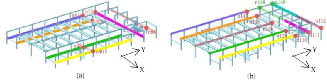
Figure 5.11 Groups of columns with uniform behavior and nodes with maximum acceleration response for a) the first level, and b) the second level. ... 58
Figure 5.12 Pushover global control analysis. (a) X direction: δy = 0.033m, δu = 0.228m, Tb = 7010 kN, (b) Y direction: δy = 0.035m, δu = 0.232m, Tb = 6480 kN, (c) comparison between pushover analysis conducted with lumped and diffused approach (x-direction) ... 60
xii
Figure 5.13 Displacements obtained from nonlinear time history analysis. (a) X-direction:
δmax = 0.155m; (b) Y-direction: δmax = 0.176m. ... 61
Figure 5.14 Evolution of damage indices during the seismic event. (a) x-direction: DIμ max = 0.626. (b) y-direction: DIμ max = 0.714. ... 61
Figure 5.15 Time histories and FFT of registered accelerograms: (a) Umbria-Marche (1997), PGA 1.69 m/sec2; (b) L’Aquila (2005) PGA 6.44 m/sec2 ... 62
Figure 5.16 Maximum displacement and damage indices obtained with real time history: (a) Umbria-Marche: X-direction δmax = 0.101; DIμ max = 0.346, (b) Umbria-Marche: Y-direction δmax = 0.093; DIμ max = 0.296, (c) L’Aquila: X-direction δmax = 0.117; DIμ max = 0.433, (d) L’Aquila: Y-direction δmax = 0.114; DIμ max = 0.403 ... 63
Figure 6.1 sensors placement, (a) AVS performed the 17/12/2015, (b) AVS performed the 18/12/2015 ... 67
Figure 6.2 Instrumentation used for each AVS: (a) CompactDAQ-9132 and NI 9234 module, (b) KS48C piezoelectric sensor 1V/g, (c) KB12VD piezoelectric sensor 10V/g ... 68
Figure 6.3 (a) stabilization diagram and (b), (c), (d), (e), (f) complexity plots of the firsts five modes identified ... 69
Figure 6.4 Particular of rigid modelled in F.E. model: (a) hidden view and (b) wireframe view ... 71
Figure 6.5 Comparison between FE model updated and ODS of AVS: (a) mode1, (b) mode2, (c) mode3, (d) mode5, (e) mode8 ... 72
Figure 6.6 Frequency correlation between AVS and FEM ... 73
Figure 6.7 Comparison between the corresponding modes of preliminarily NM (a) and the updated NM (b) ... 74
Figure 6.8 (a) External views of the Ugo Foscolo School building, (b) Plan View of floor type, (c) transversal section and d) perspective drawing of the main façade ... 76
Figure 6.9 (a) Structural plan view, (b) structural drawing of CFRP in column-beam nodes, (c) executive drawing of a column intervention, (d) October 2015, original column type and disconnection of infill panels, (e) January 2016, significant enlargement of original columns, (f) April 2016, end of retrofit phase ... 78
Figure 6. 10 Instrumentation used for each AVS: (a) Digital Recorder DaTa500, RG58 cables, Signal conditioners, (b) KB12VD piezoelectric sensor 10V/g, (c) KS48C piezoelectric sensor 1V/g ... 80
Figure 6.11 identification process of each Ambient Vibration Surveys: location of the sensors, stabilization diagrams and FFT of the most significant time histories. (a) AVS1, (b) AVS2, (c) AVS3, (d) AVS4 ... 81
Figure 6.12 Tracking of natural frequencies at each AVS ... 83
Figure 6.13 (a) Comparison between FE model updated and (b) ODS of AVS1 ... 85
Figure 6.14 (a) Comparison between FE model updated and (b) ODS of AVS2 ... 86
Figure 6.15 (a) Comparison between FE model updated and (b) ODS of AVS3 ... 87
Figure 6.16 (a) Comparison between FE model updated and (b) ODS of AVS4 ... 88
Figure 7.1 Single node hardware architecture. ... 93
Figure 7.2 Nodes components arranged in their case (left), the 3 boards stacked in "tower" configuration (right). ... 93
Figure 7.3 Sensor design ... 94
Figure 7.4 General architecture of wireless sensor network. ... 94
xiii
Figure 7.6 Floor noise of Loccioni nodes compared with a standard 1V/g piezoelectric
seismic accelerometer ... 95
Figure 7.7 Calibration setup: (a) plan view of wireless sensor, (b) orientation of sensors for X direction, (c) orientation of sensors for Y direction ... 96
Figure 7.8 Calibration curves of each sensor ... 98
Figure 7.9 Views of: (a) the south part between years 1902-1905, (b) the actual front, (c) Salone degli Stemmi, (d) International Accordion’s Museum. ...101
Figure 7. 10 (a) Architectural plan view of the ground floor, (b) transversal section of the building. ...102
Figure 7.11 Layout of the accelerometers at each floor. ...103
Figure 7. 12 Background noise of LoccioniTM accelerometer (black line) compared with an ambient vibration registered in one point of the structure (grey line): (a) acceleration time history, (b) PSD ...104
Figure 7.13 Stabilization diagram (Cov-SSI). ...105
Figure 7.14 Modal shapes identified with SSI technique. ...106
Figure 7.15 View of the FE model of the structure. ...107
Figure 7.16 Starting point of the mechanical characteristics of the main elements. ...108
Figure 7.17 Views of boundary constraints applied in the model in (a) X-direction and (b) Y-direction. ...108
Figure 7.18 The first four modes of the Numerical Model (NM): starting point for the calibration. ...109
Figure 7.19 The first four modes of the NM after the first calibration. ...111
xv
List of Tables
Table 5.1 Interpretation of damage index ... 43
Table 5.2. Mechanical characteristics of the main elements (see Fig. 5.5) ... 51
Table 5.3 Modal parameters of the structure (in bold the participation masses of the main modes) ... 52
Table 5.4 Kent and Park parameters ... 54
Table 5.5 Menegotto and Pinto parameters ... 55
Table 6.1 number and duration of performed AVS’s ... 66
Table 6.2 Results of dynamic identification: frequencies and damping ratios ... 70
Table 6.3 Comparison between analytical and experimental values of natural frequencies (in bold the calibrated frequencies and the significant participation masses) ... 72
Table 6.4 Dynamic parameters identified with Cov-SSI technique ... 82
Table 6.5 Comparison between analytical and experimental values of natural frequencies (in bold the calibrated frequencies respect to the AVS1 and the significant participation masses) ... 85
Table 6.6 Comparison between analytical and experimental values of natural frequencies (in bold the calibrated frequencies respect to the AVS2 and the significant participation masses) ... 86
Table 6.7 Comparison between analytical and experimental values of natural frequencies (in bold the calibrated frequencies respect to the AVS3 and the significant participation masses) ... 87
Table 6.8 Comparison between analytical and experimental values of natural frequencies (in bold the calibrated frequencies respect to the AVS4 and the significant participation masses) ... 88
Table 7. 1 – calibration of wireless sensors: averaged values of voltage for each each sensor (x and y directions) ... 97
Table 7.2 Sensitivity of MEMS accelerometers ... 98
Table 7.3 Modal shapes identified with Cov-SSI technique. ...105
Table 7.4 Modal properties for starting Numerical Model (NM). ...109
Table 7.5. Modal properties for starting the first calibration of NM. ...110
Table 7.6 Modal properties after the second calibration of NM. ...111
Table 7.7. Modal properties after the third calibration of NM. ...112
Table 7.8 Final modal properties of calibration of NM. ...112
Table 7.9 Comparison between analytical and experimental values of natural frequencies. ...114
Chapter 1 - Introduction
Pierdicca A. – Monitoring and Self-Diagnosis of Civile Structures: classical and innovative applications
1
Chapter 1
Introduction
In recent years the preservation of buildings and their structural safety are becoming topics of growing interest, encouraging the development of new methods and procedures for structural monitoring [1]. SHM is a set of techniques and methodologies for detection, localization, characterization and quantification of damaging phenomena. These techniques are used, among others, to predict the residual life of the structure before it reaches its collapse [2,3]. In fact, following the evolution of structural damage over time is crucial to understand if the damage mechanism has stopped and if the structure still has adequate resistance.
Seismic analyses for structural interventions are frequently performed using simplified numerical models that try to best reproduce the real dynamic behavior of the building. Often these models are not sufficiently refined and do not represent the real structure well enough. Destructive controls and structural surveys increase the knowledge of the structure, but are often not sufficient to understand the dynamic properties of the building. Due to the many uncertainties about construction systems - material properties, modelling techniques, analysis methods and successive past interventions - the evaluation of structural behavior is a difficult task. These uncertainties can be the cause of completely wrong results.
SHM techniques solve these aspects. It is defined as the use of in-situ, non-destructive sensing and analysis of structural characteristics in order to identify if damage has occurred, to define its location and to estimate its severity, to evaluate its consequences on residual life of the structure.
Nowadays the reduction of equipment cost and the increase of computational performances have made the dynamic identification process widely used in civil engineering, particularly in existing buildings. These techniques can be applied for calibration of structural models of buildings to be used for repair-oriented design, rehabilitation and retrofit works, and the structural monitoring of the building by observing changes of its dynamic behavior in time.
Operational Modal Analysis (OMA) concerns the possibility of describing structural dynamics at small vibration amplitudes in real operating conditions with unknown excitation inputs (e.g., wind force) [4]. The importance of this issue comes from the fact that for identification of large civil structures, applying known excitation forces is costly, if not infeasible [5,6]. Moreover, output only algorithms are the best option for an online monitoring system, which can monitor vibrations of a structure constantly, without the application of a measurable input to the system.
Chapter 1 - Introduction
2 Pierdicca A. - Monitoring and Self-Diagnosis of Civile Structures: classical and innovative applications
1.1 Why SHM for civil applications
“Can theoretical models correctly represent the real dynamic properties of structures?” and “How to identify and quantify the evolution of damage?” are key questions which this research proposes to answer.
The methodology normally used to solve these issues is SHM. The procedure involves: observation of a structure in a specific period using periodic measurements; extraction of specific features of the measured variables; analysis of the characteristics detected to determine the state of health of the structure. For these reasons the environmental and operating conditions have to be determined choosing the type of variable to be monitored (choice of sensors, position, data acquisition system, etc.) and the method of data acquisition (continuous, periodically, only after extreme events, etc.).
The goal of SHM is to improve safety and reliability of infrastructure systems by detecting damage before it reaches a critical state and allow rapid post-event assessment.
Early detection of damage is a fundamental task from a safety and economic point of view. Traditionally, damage detection is performed through periodic maintenance and post-event visual inspection by qualified personnel. Visual inspections impose high costs and inconvenience on structural system owners and users alike. In buildings, for instance, visual inspections may require the removal of non-structural components such as ceiling tiles, partition walls, and fire proofing. In addition, such resources (qualified inspectors) may not be immediately available after a damaging event, especially for dense urban areas, prolonging expensive downtime.
The SHM system solution offers precise information which helps engineers and managers assess the state-of-health of their structures, and if needed, target specific regions to inspect.
The dynamic behavior of civil structures can be obtained by experimental tests conducted using know input. This procedure is called Experimental Modal Analysis (EMA). It allows the identification of dynamic properties of structures by applying input-output modal identification procedures. Traditional EMA, however, suffers some limitations, such as:
- Need of an artificial excitation in order to measure Frequency Response Functions (FRF). In some cases, such as large civil structures, it is very difficult or even impossible to provide adequate excitation;
- Artificial loading is usually expensive;
- External excitation is affected by the risk of damaging the structure.
As a consequence, in the last decades increasing attention has been focused on Operational Modal Analysis. OMA is based on measurements affecting only the response of the structure in operational conditions and subject to ambient excitation in order to extract modal characteristics. It is also called “ambient”, or “output-only” modal analysis. OMA is very attractive due to a number of advantages with respect to traditional EMA:
- testing is fast and cheap to conduct;
- no excitation equipments are needed, nor boundary condition simulation; - it does not interfere with the normal use of the structure;
Chapter 1 - Introduction
Pierdicca A. – Monitoring and Self-Diagnosis of Civile Structures: classical and innovative applications
3
- it allows identification of modal parameters which are representative of the whole system in its actual operational conditions;
- operational modal identification by output-only measurements can be used also for vibration-based structural health monitoring and damage detection of structures.
On the other hand, typical drawbacks are related to a signal-to-noise ratio in measured data much lower than in the case of controlled tests in lab environment. Thus, very sensitive equipment and careful data analysis are needed.
The appeal of these techniques motivated the presented dissertation in investigating the dynamic behavior of civil structures through OMA procedures.
1.2 Thesis outline
In the present thesis, Structural Health Monitoring procedures and Operational Modal Analysis techniques for civil structures are investigated.
The first step was to study the state-of-the-art of SHM, both regarding long and short-term monitoring to try and understand the role that SHM can play in the protection and in the maintenance of ordinary buildings (Chapter 2). Chapter 3 provides a breakdown of research in Operational Modal Analysis process and the methodology used for the measuring campaign. An extensive literature review of OMA procedures is carried out, describing their theoretical background.
An overview of equipment and measurement instruments for the identification process in output-only conditions is addressed in Chapter 4. In this chapter, the hardware component (sensors, data acquisition hardware) characteristics and some practical issues are described in detail, in order to define the parameters to consider for a proper choice of hardware to be used for ambient vibration tests.
In Chapter 5, the damage detection theme is addressed and a complete literature of damage indexes is discussed. Through a case study, an integrated novel approach is proposed for the diagnosis of structures after a seismic event. The leading idea of this approach is to provide an estimation of the health and remaining life of monitored structures and to detect and quantify the damage, some of the crucial issues of SHM.
The reliability and high versatility of OMA techniques, which do not require knowledge about the excitation that causes structural vibrations, is demonstrated by applying them to a number of different case studies (Chapter 6). For each of them a modal model is obtained and dynamic parameters are extracted. Experimental data are also validated by performing suitably tuned numerical models. They allow the enhancing of structural aspects of the monitored buildings, characterizing the different parameters and boundary conditions that deeply influence the structural dynamic.
Finally, Chapter 7 investigates an alternative way to perform dynamic measurements: Wireless Sensor Networks (WSN). With respect to a wired solution a WSN is usually a flexible solution with minor associated costs, especially if the network is composed of cheap devices (e.g., MEMS sensors). On the other hand, new problems should be considered: the synchronization between sensor nodes, the short transmission distance, the optimization of energy consumption and the selection of adequate low-cost sensors. In this framework, this Chapter details the main results obtained in the context of a masonry building monitored with WSN, with the aim of obtaining an accurate numerical model that simulates
Chapter 1 - Introduction
4 Pierdicca A. - Monitoring and Self-Diagnosis of Civile Structures: classical and innovative applications
the dynamic behavior of the whole structure. The device prototype is assembled and tested, showing the sensor design, the performances and the synchronization method.
Conclusions of the present research work are summarized in Chapter 8. Furthermore, open issues and suggestions for future research in the field of vibration-based structural health monitoring are also given.
Chapter 2 – Structural Health Monitoring: State of Art
Pierdicca A. - Monitoring and Self-Diagnosis of Civile Structures: classical and innovative applications
5
Chapter 2
Structural Health Monitoring: State of art
2.1 Introduction to SHM
The most important objective in civil and earthquake engineering is to provide a structure with a proportionate margin of safety against damage due especially to significant events such as earthquakes. For this reason a control of the health condition of the structure becomes advisable and necessary for the safety of buildings [7].
In the most general terms, damage can be defined as changes introduced into a system that adversely affect its current or future performance [1]. Implicit in this definition is the comparison between two different states of the system, the initial, or undamaged state, and the ultimate, or damaged state.
The process of implementing a damage identification strategy for mechanical systems (aerospace, civil, engineering infrastructure, etc.) is referred to as SHM. This process involves the observation of a structure or mechanical system over time using periodically spaced measurements, the extraction of damage-sensitive features from these measurements and the statistical analysis of these features to determine the current state of system health.
The basic idea is that modal parameters, such as frequencies, mode shapes and modal damping, are based on the physical properties of the whole structure such as mass, damping and stiffness. So when a structure is exposed to damage the corresponding modal properties are changed. This approach is commonly called Vibration-Based SHM.
SHM is a very multidisciplinary field, where a number of different skills (seismology, electronic and civil engineering, computer science, signal theory) work together in order to increase performance and reliability of this field of research.
The first application of dynamic techniques based on the study of vibration was the rotating machinery. During the 1970s and 1980s, vibration-based damage identification methods were used for offshore platforms. This damage identification problem is fundamentally different from that of rotating machinery because the location of damage is unknown and because a large part of the structure is not readily accessible for measurement.
The aerospace community began to study the use of vibration-based damage identification during the late 1970s and early 1980s in conjunction with the development of the space shuttle.
The civil engineering community has studied vibration-based damage assessment of bridge structures and buildings since the early 1980s. Modal properties and quantities derived from these properties have been the primary features used to identify damage in bridge structures. Environmental and operating condition variability and the physical size presents significant challenges to bridge monitoring application.
Nowadays SHM techniques are widely used in civil applications and information obtained from this discipline can be useful for: (i) maintenance or structural safety evaluation of existing structures; (ii) rapid evaluation of conditions of damaged structures
Chapter 2 – Structural Health Monitoring: State of Art
6 Pierdicca A. - Monitoring and Self-Diagnosis of Civile Structures: classical and innovative applications
after an earthquake; (iii) estimation of residual life of structures; (iv) repair and retrofitting of structures; (v) maintenance, management or rehabilitation of historical structures.
2.2 SHM Classifications
The damage state of a system can be described as a five-step process along the lines of the process discussed in Rytter (1993) to answer the following questions [5]:
(i) Existence. Is there damage in the system? (ii) Location. Where is the damage in the system? (iii) Type. What kind of damage is present? (iv) Extent. How severe is the damage? (v) Prognosis. How much useful life remains?
Answers to these questions in the order presented represent increased knowledge of the damage state.
The main category of classification for damage identification distinguishes between methods based on time dependent strategies. They are characterized as short-term, long-term, periodic, continuous, and triggered monitoring [8].
- Short-term monitoring can be used to examine the state of the structure at a specific point in time. This is a typical measure if an inspection shows a deficiency or damage in the structure and the safety is questioned. These types of monitoring are often used to evaluate a change. If several short-term monitoring measures are repeated frequently over an extended period it will be defined as periodic long-term monitoring.
- Long-term monitoring definition states that continuous monitoring of a structure is considered to be “long term” when the monitoring is carried out over a period of years-to-decades. Preferably, long-term monitoring should be carried out over the life of the structure. Recent advances in sensor technology, data acquisition, computer power, communication systems, data and technologies now makes it possible to construct this type of system. Long-term monitoring should be considered if the monitored quantity changes slowly (e.g. temperature) or if the loads are not predictable (e.g. natural hazards such as floods, hurricanes or earthquakes).
- Periodic, continuous or triggered monitoring. In long-term monitoring the collection of data is periodic when data is collected at regular time intervals. Continuous monitoring is used when rapid changes due to stochastic events are expected. Triggered periodic monitoring is when data collection is triggered by a specific event, e.g. when a measured parameter exceeds a threshold. The sampling interval for each data collection depends on the dynamic nature of the studied phenomena. A typical application for triggered monitoring is measurements of earthquake time histories. Another important classification of SHM approach is based on the width of the structure involved.
- Local monitoring is the observation of local phenomenon, such as strain or crack opening. Local monitoring is not able to determine the health of the whole structure.
Chapter 2 – Structural Health Monitoring: State of Art
Pierdicca A. - Monitoring and Self-Diagnosis of Civile Structures: classical and innovative applications
7
Still, in combination with global monitoring methods, local monitoring approach can be a useful to evaluate the severity of detected damages.
- Global monitoring is defined as the observation of global phenomena of structures. A typical application is the monitoring of modal parameters, such as frequencies, mode shapes and damping of the structure and to correlate the test results with the outcome of FE-analysis. The challenge is then to create a “damaged” FE-model so that the monitored results comply with the FE-analysis.
The last fundamental classification is based on the sampling rate of the measurement. - Static monitoring is used for measurements of phenomena such as deflection,
inclination, settlements, crack widths, temperature, and humidity. These are quasi-static since they vary slowly over the time.
- Dynamic monitoring is performed with a much higher sampling rate compared to static monitoring. It is usually used for measurements of accelerations in order to control the dynamic structural response.
For long-term SHM, the output of this process is periodically updated. Under an extreme event, such as an earthquake, SHM is used for rapid condition screening. This screening could provide, in near real-time, reliable information about system performance during such extreme events and the subsequent integrity of the system.
2.3 SHM applications
In conjunction with evolution, miniaturization and cost reductions of digital computing hardware developments, SHM has received considerable attention in the technical literature and practical applications. There are many real-life SHM studies in the USA, Japan, Hong Kong and Europe. New advances in sensor and information technologies and the wide use of the Internet make SHM a promising technology for better management of such civil infrastructures. Large-scale, real-life studies have been presented at a number of specialty conferences and workshops.
SHM for civil implementation can assist in the planning during the construction phase. The main objective for applying SHM to new structures is to provide feedback during erection and construction. Monitoring may help to manage safety risks during construction, as incomplete structural systems are typically vulnerable and exposed to accidents and hazards. Design of instrumentation and data acquisition for monitoring the construction process is best accomplished before the construction drawings and specifications are finalized. In fact, it is highly desirable to integrate monitoring directly into the design specifications. In this manner, the validity of the assumptions made during design calculations regarding the forces, reactions, displacements and drifts that a structure is expected to experience during its construction can be checked and confirmed. If the measurements indicate a need to modify the erection and construction, appropriate steps may be taken in a timely manner. Monitoring may therefore help to mitigate the uncertainties. The risk of constructing a structure with undesirably high forces, deformations and any other initial defects may be controlled. In addition, the design of fabrication monitoring before the start of construction may serve as an excellent measure for checking and mitigating any omission or errors in the executive drawings.
SHM is also a useful tool for evaluating the health conditions of existing buildings. It allows to make decisions for continued use, maintenance/repair/retrofit of aged or
Chapter 2 – Structural Health Monitoring: State of Art
8 Pierdicca A. - Monitoring and Self-Diagnosis of Civile Structures: classical and innovative applications
damaged structures. SHM application may be made in the case of existing structures that exhibit premature aging, distress and performance problems. Some structures may lack sufficient system reliability due to undesirable construction details. In this case, the challenge would be to design a retrofit that would provide a significant enhancement of the system reliability. The analysis and interpretation of such data would provide critical information about the current load and responses as well as remaining fatigue life.
SHM can also be applied to large populations of similar types of structures. This kind of approach offers great promise for the implementation of structures by fully and systematically capitalizing on the common threads in the behavior of structures types. The science of statistical sampling, applied in conjunction with structural identification and structural health monitoring, would permit civil structures to be grouped into populations with similar behaviors. Some representative parameters can be monitored to evaluate the performance and health. Any findings such as root causes for damage and deterioration obtained from the SHM applications can be considered for the entire population when large-scale decisions are to be made.
2.4 SHM general methods
For any SHM application, it is imperative to properly-define the needs, requirements, expectations and constraints of the monitoring project. The expected outcome of the monitoring program should be clearly identified and analyzed, providing answers to specific questions such as load rating, structural behavior or performance.
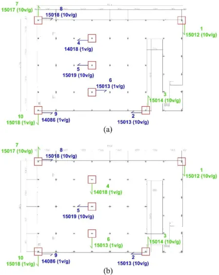
As clearly summarized by Catbas F.L et al. [9], once the overall objectives and expectations are established, the following critical issues need to be considered (Fig.2.1).
Figure 2.1 Simplified representation of stages involved in SHM process [10]
Structural system characterization. Characterization leads to a deep understanding of the structure and the objectives of the monitoring application. First, a thorough review is to be conducted using any relevant design information and drawings. Development of
Chapter 2 – Structural Health Monitoring: State of Art
Pierdicca A. - Monitoring and Self-Diagnosis of Civile Structures: classical and innovative applications
9
analytical or Finite Element Models (FEM) for simulation of structural response is to be considered for structural characterization. These models also assist in the design of the monitoring project. Such models may be further refined and calibrated using SHM data to reflect actual conditions and mechanisms, and can serve as a baseline for evaluating future changes in the condition, performance and health of the structure.
Identifying the measurements. Based on the SHM objectives and characterization of the system, measurement needs have to be identified. The individual mechanical, chemical, electrical, and optical parameters that will characterize the phenomena of interest are to be evaluated. These parameters can include forces, stresses, displacements, rotations, vibrations, distortions and strains, environmental parameters such as temperature, humidity, precipitation, wind speed and direction, traffic quantities, images, etc. Some parameters may be static in nature, while others may be dynamic.
Sensing and data acquisition system selection. A detailed set of installation specifications should be prepared for each type of sensor and data acquisition component that will be used. These specifications should detail the methods and techniques to be used for installing and configuring the sensors and data acquisition components, and a methodology for verifying that they are working correctly.
Data quality assurance, processing and archival. Developing appropriate methods for data quality assurance, processing and archival purposes represent the major information technology related challenges for SHM applications. There are many possible sources of error and uncertainty in the field that can affect the reliability of measurements. Therefore, it is often desirable to have the methods developed and implemented at multiple levels of the signal path for quality assurance.
Data presentation and decision-making. The final step in the design process is to develop criteria for interpreting and presenting the monitor data and for making subsequent decisions. A monitoring system should generally only display data that have been synthesized to a form that is meaningful and can be easily understood. In a long-term structural health monitoring application, the system should be able to interpret the measurement data, compare the result with some predetermined set of criteria, and make a decision in an automated manner. The simplest example is to program a health monitoring system to issue an alert when the measurement data indicate that some behavior has exceeded a particular threshold value.
The procedure can be used to forecast the lifetime of the structure that was useful for the so-called Process of Prognosis, in order to predict the remaining life of the structure examined.
Chapter 2 – Structural Health Monitoring: State of Art
Chapter 3 – Output-Only Modal Identification
Pierdicca A. - Monitoring and Self-Diagnosis of Civile Structures: classical and innovative applications
11
Chapter 3
Output-Only Modal Identification
3.1 Introducing OMA
The dynamic behavior of physical systems is often described by defining an ideal constant-parameter linear system (also known as Linear Time-Invariant—LTI—system, Fig.3.1). A system is characterized by constant parameters if all its fundamental properties are invariant with respect to time. Moreover, it shows a linear mapping between input and output if the response characteristics are additive and homogeneous.
Figure 3.1 Schematic illustration of LTI system
For real structures, the validity of the linearity assumption depends not only on the characteristics of the structure, but also on the magnitude of the input. Physical systems typically show non-linear response characteristics when the magnitude of the applied load is large. However, for the applications of our interest, the response of many structures can be reasonably assumed to be linear, since ambient excitation yields small amplitude vibrations.
From a general point of view, the dynamics of a civil structure, like any mechanical system, can be described in terms of its mass, stiffness, and damping properties, or in terms of its vibration properties (natural frequencies, damping ratios, and mode shapes) or in terms of its response to a standard excitation.
Other descriptors of the dynamics of constant-parameter linear systems are defined in terms of their response to “standard” excitations. When the excitation is represented by a unit impulse input, the dynamics of the system can be described by its impulse response function (IRF). When the excitation is a unit-amplitude sinusoidal force applied at every frequency in a given range, another descriptor is obtained: it is the so-called frequency response function (FRF) defined over the considered range of frequency.
Consider for simplicity a Single Degree of Freedom (SDOF) system (the concepts can be easily extended to general MDOF systems by appropriate matrix notation). For any arbitrary input , the output of the SDOF system is given by the following convolution integral of the IRF ℎ with the input:
Chapter 3 – Output-Only Modal Identification
12 Pierdicca A. - Monitoring and Self-Diagnosis of Civile Structures: classical and innovative applications
Alternatively, a physically realizable and stable LTI system can be described by the FRF . The convolution integral reduces to a simple multiplication when it is expressed in terms of the FRF and the Fourier Transforms of the input and the output :
= 3.2
By solving the equations of motion when harmonic forcing is applied, the complete solution is described by a single matrix known as the Frequency Response Matrix .
The system characteristics are completely contained in , which can be easily computed from:
= 3.3
This procedure is called Experimental Modal Analysis (EMA) and is usually performed when both the input and the output signals are known.
For a random excitation, a different approach is required. In this case the input is unknown and the only known variable is the output . Moreover, when both excitation and response are described by random process, neither excitation nor response signals can be subjected to a valid Fourier Transform calculation and another approach must be found. As input is unknown, it is assumed to be a stationary zero mean Gaussian white noise: this assumption implies that input is characterized by a flat spectrum in the frequency range of interest and, therefore, it gives a broadband excitation, so that all modes are excited. As a consequence, the output spectrum contains full information about the structure, since all modes are equally excited.
For these reasons it is necessary to introduce and define different identification approaches. This procedure, previously introduced, is called Operational Modal Analysis (OMA).
OMA techniques are based on the following assumptions:
- Linearity: the response of the system to a certain combination of inputs is equal to the same combination of the corresponding outputs;
- Stationarity: the dynamic characteristics of the structure do not change over time, that is to say, coefficients of differential equations describing the problem are constant with respect to time;
- Observability: test setup must be defined in order to be able to measure the dynamic characteristics of interest (nodal point must be avoided in order to detect a certain mode).
OMA is the base for a number of applications: in particular, it is currently used in vibration-based structural health monitoring systems, founded on the relation between damage and changes in structural properties, such as mass, damping and stiffness.
The general procedure involves three stages. First, to identify the appropriate type of model (the Spatial Model) in terms of mass, stiffness and damping properties. Second, an analytical modal analysis of the Spatial Model is performed. It describes the structural behavior as a set of natural frequencies with corresponding vibration mode shapes and modal damping factors (the Modal Model). The third stage is characterized by the analysis of the structural vibration under given excitation conditions to describe the Response
Chapter 3 – Output-Only Modal Identification
Pierdicca A. - Monitoring and Self-Diagnosis of Civile Structures: classical and innovative applications
13 Model. This will depend not only upon the properties of the structure but also on the nature
and magnitude of the imposed excitation.
Processing of the Modal Model passes through the following steps:
- planning and execution of tests (proper location of sensors and, eventually, of actuators; selection of data acquisition parameters; eventual application of external excitation);
- data processing and identification of modal parameters (filtering, decimation, windowing; extraction of modal parameters);
- validation of the modal model.
Once the modal model has been found, it can be used for different purposes. A first approach is based on the observation that changes in structural properties have
consequences on natural frequencies. However, their relatively low sensitivity to damage
requires high accuracy of measurements in order to obtain reliable results. Significant changes in modal frequencies could not necessarily imply presence of damage, because of the effects of some environmental factors such as temperature changes. A variation of about 5% seems to be necessary to detect damage with confidence.
Damage can be detected through mode shape changes. A number of applications are reported in the literature but the most popular ones are based on some indexes such as Modal Assurance Criterion (MAC) [11].
Another important application of system identification, which is in some way related to the issues of monitoring and damage prognosis, is force reconstruction: in fact, knowledge of loads acting on structures gives opportunities in the field of structural health assessment and of estimation of the remaining lifetime. In many practical applications it is impossible to measure forces resulting, as an example, from wind or traffic directly. Therefore, they can be determined only indirectly from dynamic measurements. All these methods require system identification as a first step for load estimation.
The last main application of results of modal analysis concerns model updating. The extracted modal parameters can be used to validate or enhance numerical models. In fact, FE models are usually affected by errors and uncertainties. If a quite accurate model is available and there is some a-priori knowledge about characteristics of the structure or materials, it is possible to carry out sensitivity analyses on the remaining uncertain parameters in order to identify the values associated to the “best model”. Usual applications of FE model updating aim at identifying material properties or boundary conditions. Several techniques for model updating exist, including manual tuning of the update parameters. The updated model can be used for damage detection purpose [12] or for evaluation of short-term impact of natural hazardous events (earthquakes) or rehabilitation and retrofitting works.
In the next sections, after a short review about models of vibrating structures, the basic theory underlying the different OMA methods will be presented.
Chapter 3 – Output-Only Modal Identification
14 Pierdicca A. - Monitoring and Self-Diagnosis of Civile Structures: classical and innovative applications
3.2 Structural Dynamics Models
3.2.1 Equation of motion and structural dynamic properties
The dynamic behavior of a structure can be represented either by a set of differential equations in time domain, or by a set of algebraic equations in frequency domain. Equations of motion (Fig 3.2) are traditionally expressed in time domain, thus obtaining, for a general MDOF system, the following set of linear second order differential equations expressed in matrix form:
+ + = 3.4
where , and are the vectors of acceleration, velocity, and displacement, respectively; , , and denote the mass, damping, and stiffness matrices; is the forcing vector.
Figure 3.2 Schematic illustration of MDOF system
It describes the dynamics of the N-DOF discrete DOFs of the structure and it is usually referred to as the spatial model. The definition of the spatial model (of mass, stiffness, and damping properties) is the first step in theoretical analyses and it usually requires a large number of DOFs (some order of magnitude larger than the number of DOFs required for an accurate experimental model) in order to adequately describe the dynamic behavior of the structure.
Frequencies, damping and mode shapes are obtained by the associated homogeneous equation:
+ + = 0 3.5
in addition, the solution is harmonic:
= 3.6
Eigenproblem associated to , , and matrix is obtained by substituting (3.6) in (3.5):
Chapter 3 – Output-Only Modal Identification
Pierdicca A. - Monitoring and Self-Diagnosis of Civile Structures: classical and innovative applications
15
+ + = 0 3.7
Through the calculation of (3.7) N eigenvalues and N eigenvectors, in general complex entities, are obtained. Usually eigenvalues can be rewritten as [13]:
= − + 1 − 3.8
Where is the jth natural frequency in undamped system, and is the associated modal damping.
3.2.2 State space models
State space-models are used to convert the second order problem, stated by the differential equation of motion (3.4) in matrix form, into two first order problems, defined by the so-called “state equation” and “observation equation”. The state equation can be obtained by the second order equation of motion and can be conveniently given by:
= + 3.9
obtained by introducing in (3.4) the state vector , the “state matrix” , the “input influence matrix” and the external force vector defined as follows:
=
= − 0 −
= 0
= 0
where the subscript “c” denotes continuous time. The system (3.8) is composed by 2N first-order differential equation.
Real structures are characterized by an infinite number of DOFs which becomes a finite but large number in finite element models, where lumped systems are considered. However, in a practical vibration test, this number decreases from hundreds and hundreds to a few tens or even less. Thus, by assuming that measurements are taken at “L” locations and that the sensors are either accelerometers, velocimeters and displacement transducers in the most general case, the state equation can be associated with the observation
equation:
Chapter 3 – Output-Only Modal Identification
16 Pierdicca A. - Monitoring and Self-Diagnosis of Civile Structures: classical and innovative applications
where is the vector of the outputs, , and are the output location
matrices for acceleration, velocity and displacement respectively.
Combining equations (3.4) and (3.10) the following equation can be written:
= + 3.11
obtained by introducing the following definitions:
= − −
=
= 0
where is the “output influence matrix” (Lx2N) and is the “direct transmission
matrix” (LxN). The direct transmission matrix disappears if no accelerometers are used for
output measurements.
By combining equations (3.9) and (3.11), the classical continuous-time state-space
model is obtained:
= +
3.12
= +
Since experimental tests yield measurements taken at discrete time instants while equations (3.12) are expressed in continuous time, the state space model must be converted to discrete time. By choosing a certain fixed sampling period ∆ , the continuous-time equations can be discretized and solved at all discrete continuous-time instants = ∆ , obtaining the discrete-time state-space model formulation:
= +
3.13
= +
Where = ∆ is the discrete-time state vector yielding the sampled displacements and velocities, and are the sampled input and output, [ ] is the discrete state matrix, [ ] is the discrete input matrix, [ ] is the discrete output matrix and [ ] is the direct transmission matrix.
Once the state space model has been constructed, the modal parameters can be extracted by the eigendecomposition of the system matrix , as described in Section 3.4.2.
Chapter 3 – Output-Only Modal Identification
Pierdicca A. - Monitoring and Self-Diagnosis of Civile Structures: classical and innovative applications
17
3.3 Characterization of Output-Only techniques
Even if most of OMA techniques are derived from traditional EMA procedures, they are developed in a stochastic framework, due to the assumptions about input. Such assumptions have some consequences: first, modal participation factors cannot be computed as the input is unknown; moreover, due to the assumptions on input, OMA techniques are always of a multiple input type.
Modal identification methods can be first of all classified according to the domain for implementation. Parameter estimation methods directly based on time histories of the output signals are referred to as time domain methods. Methods based on Fourier transform of signals are, instead, referred to as frequency domain methods.
Time domain methods are, in fact, usually better conditioned than the frequency domain counterpart. This is mainly related to the effect of the powers of frequencies in frequency domain equations. Moreover, time domain methods are usually more suitable for handling noisy data, and they avoid most signal processing errors if applied directly to raw time domain data. On the other hand, in noisy measurement conditions, averaging is easier and more efficient in the frequency domain.
A second distinction is between parametric and non-parametric methods; if a model is fitted to data, the technique is called parametric. These procedures are more complex and computationally demanding compared to non-parametric ones, but they usually show better performance with respect to the faster and easier non-parametric techniques which, however, give a first insight into the identification problem.
A third distinction is between Single Degree Of Freedom (SDOF) and Multiple Degree
Of Freedom (MDOF) methods. If in a certain frequency band only one mode is assumed to
be important, the parameters of this mode can be determined separately, leading to the so-called SDOF methods. Even if these methods are very fast and characterized by a low computational burden, the SDOF assumption is a reasonable approximation only if the modes of the system are well decoupled. MDOF methods are, therefore, necessary when dealing with close-coupled modes or even coincident modes.
The last distinction is among covariance-driven and data-driven methods: in the first case correlation functions are estimated from the measured responses before carrying out modal identification; in the second case modal analysis is carried out directly on the raw data.
3.3.1 OMA in frequency domain
The easiest method for modal parameter estimation from output-only data is the Basic
Frequency Domain (BFD) technique [14], also called the Peak-Picking method. The name of
the method is related to the fact that natural frequencies are determined as the peaks of the Power Spectral Density (PSD) plots, obtained by converting the measured data to the frequency domain by the Discrete Fourier Transform (DFT). The BFD technique is a SDOF method for OMA: in fact, it is based on the assumption that, around a resonance, only one mode is dominant.
The BFD technique works well when damping is low and modes are well-separated: if these conditions are violated it may lead to erroneous results. Another important drawback is that the selection of eigenfrequencies can become a subjective task if the spectrum peaks are not very clear. Moreover, eigenfrequencies are estimated on a local basis (local
Chapter 3 – Output-Only Modal Identification
18 Pierdicca A. - Monitoring and Self-Diagnosis of Civile Structures: classical and innovative applications
estimate) by looking at single spectra. The last drawback is the need of a fine frequency resolution in order to obtain a good estimation of the natural frequency.
The Enhanced Frequency Domain Decomposition (FDD) technique [15] is an extension of the BFD technique. The input x(t) and the output y(t) can be written in the form:
= ∗ 3.14
where is the “r x r” input PSD matrix, “r” is the number of inputs,
“l x l” output PSD matrix, “l” is the number of outputs, is the “l x r” FRF matrix, and the superscripts * and “T” denote complex conjugate and transpose respectively. The FRF matrix can be expressed in a typical partial fraction form in terms of poles and residues
:
= = ∑ + ∗∗ 3.15
= − + 3.16
being “n” the number of modes, the pole of the kth mode, the modal damping (decay constant) and the damped natural frequency of the kth mode. is the residue, and it is given by:
= 3.17
where is the mode shape vector and is the modal participation vector. Combining equations (3.14) and (3.15) and assuming that input is random both in time and space and has a zero mean white noise distribution (that is to say, its PSD matrix is a constant: : = ), the output PSD matrix can be written as:
= ∑ ∑ + ∗ ∗ +
∗
∗ 3.18
As reported in [15] the estimate of the output PSD know at discrete frequency = is decomposed by taking the Singular Value Decomposition (SVD) of the matrix:
j = 3.19
where the matrix is a unitary matrix holding the singular vector and is a diagonal matrix holding the scalar singular values .
The singular values, a function of the varying frequency, are assumed as a modal indicator. Under some assumptions (white noise excitation, low damping and orthogonal mode shape for close modes) it can be shown that the singular value curves in the frequency domain belonging to the diagonal of are autospectral density functions of a (SDOF) system with the same frequency and damping as the structure vibration modes. Thus, the peaks of the singular value curve, in the frequency domain, allow the identification of the system frequencies, whereas the singular vectors at the peaks estimate the corresponding mode shape. The damping ratio is determined from the Inverse Fourier Transform of the
Chapter 3 – Output-Only Modal Identification
Pierdicca A. - Monitoring and Self-Diagnosis of Civile Structures: classical and innovative applications
19
autospectral density function of the SDOF by applying the method of the logarithmic decrement [4].
More details about frequency-domain identification methods can be found in [16]. In the next section, instead, attention is focused on time-domain methods, used in several case studies presented in the present dissertation.
3.3.2 OMA in time domain
Time domain models are a powerful analytical tool for the description and interpretation of stochastic processes deriving from the observation of dynamic phenomenon. These models are initially developed in fields of system theory and control engineering. The main characteristics and basic fundamentals are described in [17,18].
In the last decades these models have been used by several researchers for dynamic identification of structural systems (bridge, buildings, etc.) subjected to environmental loads. Dynamic response acquired during experimental tests can be considered as discrete-time series and can be described in a statistical manner by stochastic processes.
Mathematical models are represented by differential equations with discrete-time variables, which coincide to differential equations corresponding to continuous-time systems. These models can be divided in two main groups: input-output models and
state-space models. The former consider the observed variables (input variables and output
variables). State-space models use auxiliary variables, called state-space variables.
In order to evaluate modal properties of the structures modal models have to be solved searching model coefficients.
Prediction Error method (PEM) allows the estimation of dynamic parameters by a
“predictor function” that provides, knowing the time history up to time instant t, the best accuracy estimation of the time history up to time instant t+1. It is then possible to obtain the coefficients by iterative optimization non-linear procedure. The so-called “predictor error function” is defined by the difference between the output signal (e.g. measured acceleration of the structure) respect to the signal predicted by the model.
State-space models, that will be debated in the next paragraphs, can be conveniently solved by subspace algorithm. Dynamic identification by subspace methods [19] is usually based on manipulation of matrix using linear algebraic operations.
The name “subspace methods” reflects that the matrix containing the measured signal can be interpreted as a vectorial space where the columns of this matrix represent a base of vectors. These matrixes can be evaluated through the only knowledge of the output, without the a-priori knowledge of the matrix of the model [20].
The prediction of the signal, necessary for the determination of the system matrix, is associated with the development of the Kalman filter [21].
The last step of the identification process is the validation of the modal model.
3.4 Stochastic Subspace Identification
In the present work modal identification is carried out through Subspace methods. For this reason a deep argumentation of these techniques is reported, omitting the mathematical presentation of other procedures.
The model given by (3.12) is a deterministic model, that is to say the system is driven only by a deterministic input. However, stochastic components must be necessarily
Chapter 3 – Output-Only Modal Identification
20 Pierdicca A. - Monitoring and Self-Diagnosis of Civile Structures: classical and innovative applications
included in order to describe actual measurement data (external random input as wind, traffic, earthquake, etc.). If stochastic components are included in the model, the following “discrete-time combined deterministic-stochastic state-space model” is obtained:
= + +
3.20
= + +
where is the “process noise” due to disturbances and model inaccuracies, while is the “measurement noise” due to sensor inaccuracy.
These vector signals are both unmeasurable: they are assumed to be zero mean Gaussian white noise processes. Due to the lack of information about the input , it is implicitly modelled by the noise terms and , thus obtaining the following “discrete-time stochastic state-space model”:
= +
3.21
= +
The equation (3.21) can be interpreted as a model where the forcing function is white noise. In this case the terms [ ] and [ ] of the equations (3.20) can be included in the terms
and obtaining the formulation (3.21).
The white noise assumption about and cannot be omitted for the proof of this class of identification methods [19]. If this assumption is violated, that is to say the input includes white noise and some additional dominant frequency components, these components will appear as poles of the state matrix [ ] and cannot be separated from the eigenfrequencies of the system.
Thus, when a stochastic state-space model is adopted, the objective is the determination of the order n of the unknown system and of a realization of the matrices [ ] and [ ] (up to within a similarity transformation) from a large number of measurements of the output generated by the system itself. The state matrix [ ] transforms the current state of the system in the next state , while the product of the observation matrix [C] with the state vector provides the observable part of the dynamics of the system.
When dealing with discrete-time stochastic state-space models, where the input is implicitly modelled by disturbance, an alternative model, the so-called “forward innovation
model” can be obtained by applying the steady-state Kalman filter to the stochastic
state-space model (3.20). In order to describe this model, some concepts about Kalman filter are reported, together with definitions of “state prediction error” and “innovation”.
3.4.1 The Kalman filter
The stochastic state-space model in can be expressed in an alternative form through the introduction of the so-called Kalman filter.
The process noise and the measurement noise and are both immeasurable and they are assumed to be zero mean, stationary white noise processes with covariance matrices given by:
![Figure 2.1 Simplified representation of stages involved in SHM process [10]](https://thumb-eu.123doks.com/thumbv2/123dokorg/2971119.27306/24.892.242.650.672.951/figure-simplified-representation-stages-involved-shm-process.webp)