Supporting Service Differentiation with Enhancements of the IEEE 802.11 MAC Protocol: Models and Analysis

UNIVERSITY

OF TRENTO

DEPARTMENT OF INFORMATION AND COMMUNICATION TECHNOLOGY 38050 Povo – Trento (Italy), Via Sommarive 14

http://www.dit.unitn.it

SUPPORTING SERVICE DIFFERENTIATION WITH

ENHANCEMENTS OF THE IEEE 802.11 MAC PROTOCOL: MODELS AND ANALYSIS

Bo Li and Roberto Battiti

May 2003

1

Supporting Service Differentiation with Enhancements of the IEEE 802.11

MAC Protocol: Models and Analysis

Bo Li and Roberto Battiti

Department of Computer Science and Telecommunications, University of Trento, 38050 POVO Trento, Italy e-mail: {li, battiti}@dit.unitn.it

Abstract. As one of the fastest growing wireless access technologies, Wireless LANs must evolve to support adequate degrees of service differentiation. Unfortunately, current WLAN standards like IEEE 802.11 Distributed Coordination Function (DCF) lack this ability. Work is in progress to define an enhanced version capable of supporting QoS for multimedia traffic at the MAC layer. In this paper, we aim at gaining insight into three mechanisms to differentiate among traffic categories, i.e., differentiating the minimum contention window size, the Inter-Frame Spacing (IFS) and the length of the packet payload according to the priority of different traffic categories. We propose an analysis model to compute the throughput and packet transmission delays. In additions, we derive approximations to get simpler but more meaningful relationships among different parameters. Comparisons with discrete-event simulation results show that a very good accuracy of performance evaluation can be achieved by using the proposed analysis model.

Keyword: Wireless LAN, IEEE 802.11 MAC, Service Differentiation, Performance Evaluation

I.Introduction

The main objective of the next-generation broadband wireless networks is to provision seamless multimedia services to mobile users. In this context, one of the major challenges of the wireless mobile Internet is to provide suitable levels of Quality of Service over IP-based wireless access networks [1]. Current approaches to provide IP QoS include IntServ [2] and DiffServ [3] architectures. The IntServ architecture defines mechanisms for per-flow QoS management and provides tight performance guarantees for high priority flows, while the DiffServ architecture defines aggregated behavior for a limited number of performance

classes for which only statistical differentiation is provided, therefore achieving better scaling performance. Wireless access may be considered just another hop in the communication path for the whole Internet. Therefore, it is desirable that the architecture supporting quality assurances follows the same principles in the wireless networks as in the wireline Internet, assuring compatibility between the wireless and wireline parts. A good example for such a wireless technology is the IEEE 802.11 Distributed Coordination Function (DCF) standard [4], which is compatible with the current best-effort service model of the Internet.

In the literature, performance evaluation of 802.11 has been executed by using simulation [5] or by means of analytical models [6]-[11]. Constant or geometrically distributed backoff window sizes have been considered in [6], [7], and [8]. In [9], an exponential backoff with only two stages is modeled by using a two-dimensional Markov chain. In [10], a more general model that accounts for all the exponential backoff protocol details is proposed. In [11], instead of using stochastic analysis, the average value for a variable is used, which results in an approximate but effective analysis.

In order to support different QoS requirements for various types of service, a possibility is to support differentiation in the IEEE 802.11 MAC layer, as proposed in [12] - [15]. In [12], a simple priority scheme for IEEE 802.11 has been proposed, where a high priority station has a shorter waiting time when accessing the medium. In [13], a service differentiation scheme is proposed. The scheme uses two parameters of IEEE 802.11 MAC, the backoff interval and the IFS between each data transmission, to provide the differentiation. In [14], service differentiation is supported by setting different minimum contention windows for different types of services. The effectiveness is demonstrated by simulation. The work in [15] proposes three service differentiation schemes for IEEE 802.11 DCF. The first one is based on scaling the contention window according to the priority of each flow. The second one assigns different Inter-Frame Spacings to different traffic classes. The third one uses different maximum frame lengths. Moreover, an effective Contention Window (CW) resetting scheme to enhance the performance of IEEE 802.11 DCF is analyzed in [16], by extending the model proposed in [10]. In [17], both the Enhanced Distributed Coordination Function (EDCF) and the Hybrid Coordination Function (HCF), defined in the IEEE 802.11e draft are evaluated through simulation.

In order to gain a deeper insight into the modified IEEE 802.11 MAC with service differentiation support, system modeling and performance analysis are needed. By building on previous papers dealing with the analysis of the IEEE 802.11 MAC, we propose an

analysis model to compute the throughput and packet transmission delays in a WLAN with Enhanced IEEE 802.11 Distributed Coordination Function, with support for service differentiation. In our analytical model, service differentiation is supported by differentiating the contention window size, the Inter-Frame Spacing, and the packet length according to the priority of each traffic flow.

The paper is organized as follows: in Section II a brief description on the IEEE 802.11 DCF and enhancements is given. In Section III the model is defined and system performance measures, i.e., throughput and average packet delays, are obtained. In Section IV, some approximations are considered to obtain simpler formulas allowing a deeper insight into the system. Then, discrete-event simulation and numerical results obtained from the analysis are presented and discussed in Section V.

II. IEEE 802.11 Distributed Coordination and Enhancements

In the 802.11 MAC sub-layer, two services have been defined: the Distributed Coordination Function (DCF), which supports delay insensitive data transmissions, and the optional Point Coordination Function (PCF), based on polling and intended to support delay sensitive transmissions. The basic 802.11 MAC protocol, the Distributed Coordination Function (DCF), works as listen-before-talk scheme, based on Carrier Sense Multiple Access (CSMA) with a Collision Avoidance (CA) mechanism to avoid collisions that can be anticipated if terminals are aware of the duration of ongoing transmissions (“virtual carrier sense”). Following is a brief summary of the DCF protocol.

When the MAC receives a request to transmit a frame, a check is made of the physical and virtual carrier sense mechanisms. If the medium is not in use for an interval of DIFS, the MAC may begin transmission of the frame. If the medium is in use during the DIFS interval, the MAC selects a backoff time and increments the retry counter. The backoff time is randomly and uniformly chosen in the range(0,W −1), W being the contention window. The MAC decrements the backoff value each time the medium is detected to be idle for an interval of one slot time. The terminal starts transmitting a packet when the backoff value reaches zero. When a station transmits a packet, it must receive an ACK frame from the receiver after SIFS (plus the propagation delay) or it will consider the transmission to have failed. If a failure happens, the station reschedules the packet transmission according to the given backoff rules. If there is a collision, the contention window is doubled, and a new backoff interval is

selected. At the first transmission attempt, W is set equal to a value CW_min called minimum contention window. After each unsuccessful transmission, W is doubled, up to a maximum value CW_max =2m⋅CW_min.

The above-described two-way handshaking technique for the packet transmission is called

basic access mechanism. Furthermore, in order to overcome the hidden station problem,

802.11 defines an optional Request-to-send/Clear-to-send (RTS/CTS) mechanism. In the RTS/CTS mechanism, before transmitting a data frame, the sender sends a short RTS frame. On receiving the RTS frame, the receiver transmits a CTS frame immediately. The RTS and CTS frames include information about the time required to transmit the next data frame, i.e., the first fragment, and the corresponding ACK response. Therefore, other stations close to the sender and hidden stations close to the receiver will not start any transmission during the advertised frame transmission period. In the paper, only the basic access mechanism is analyzed. The analysis method can be easily extended to the case of RTS/CTS access

mechanism.

The basic DCF method is not appropriate for handling multimedia traffic requiring guarantees about throughput and delay. Because of this weakness, task group E of the IEEE 802.11 working group is currently working on an enhanced version of the standard called IEEE 802.11e. The goal of the extension is to provide a distributed access mechanism capable of service differentiation. A new access mechanism called Enhanced DCF (EDCF) has been selected [18]. It is shown by simulation that EDCF has better performance than PDF, and is more scalable [19]. In this paper, in the interest of conciseness, we are not interested in exploring all details of the new proposed standard but to gain insight into three of the building block used to achieve differentiation, i.e. differentiating the minimum contention window sizes, the Inter-Frame Spacing (IFS) and the lengths of packet payload according to the priority of each traffic category.

III. Performance Analysis

A. System Modeling

We assume that the channel conditions are ideal (i.e., no hidden terminals and capture) and that the system operates in saturation: a fixed number of traffic flows always have a packet available for transmission.

different types of traffic are considered with n_i traffic flows for traffic of type i (i=1,2). We assume that type-1 traffic has a higher priority than type-2 traffic. Let b_i(t) be the stochastic process representing the backoff time counter for a given traffic flow with typei(i=1,2). Moreover, let us define for convenience Wi =CWmin,i as the minimum contention window for traffic typei. Let m_i, “maximum backoff stage” be the value such that CW _i =₂mi⋅W_i

max, . Let

) (t

s_i be the stochastic process representing the backoff stage (0,1,...,m_i) for a given traffic flow with type i. Let DIF_i denote the length of the distributed inter-frame space (DIF) of traffic flows with type i. σ is the duration of an empty slot time. Moreover, we define

σ 1

2 DIF

DIF

D≡ − as the difference between DIF₂ and DIF₁ measured in the number of empty slots. In this paper, it is assumed that DIF2 ≥DIF1. Moreover, we only consider the

case that D is an integer.

The key approximation in the model is that, at each transmission attempt for a traffic flow of type i, regardless of the number of retransmissions suffered, each packet collides with constant and independent probability p_i. This assumption has been shown by simulation to be very accurate if W_i and n_i are large [10]. The parameter p_i is referred to as conditional collision probability, the probability of a collision seen by a packet belonging to a traffic flow with type i at the time of its being transmitted on the channel. We do not assume that p1 = p2.

Later, our analysis results justify this assumption.

In the following, we use a two-dimensional discrete-time Markov chain to model the behavior of a traffic flow with type 1. The states are defined as the combinations of two integers {s₁(t),b₁(t)}. The Markov chain can be presented as follows (see Fig.1a)

Case 1: Before packet transmissions,

]) , 0 [ ], 2 2 , 0 [ ( 1 } 1 , | , {j k j k k W₁ j m₁ P + = ∈ j⋅ − ∈ (1.1)

Case 2: After packet transmissions,

− ∈ ∈ − = − ⋅ ∈ = − ⋅ ∈ ∈ = + + + ) 3 . 2 ( ]) 1 , 0 [ ], , 0 [ ( ) 1 ( } 0 , | , 0 { ) 2 . 2 ( ]) 1 2 , 0 [ ( 2 } 0 , | , { ) 1 . 2 ( ]) 1 2 , 0 [ ), , 0 [ ( 2 } 0 , | , 1 { 1 1 1 1 1 1 1 1 1 1 1 1 1 1 1 1 1 W k m j W p j k P W k W p m k m P W k m j W p j k j P m m j j

Equation (1.1) accounts for the fact that the backoff time is decremented at the beginning of each slot time. Equation (2.1) accounts for the fact that a collision occurs and the station doubles the backoff time. Equation (2.2) models the fact that once the backoff stage reaches the valuem1, it is not increased in subsequent packet transmissions. Equation (2.3) accounts

for the fact that a new packet following a successful packet transmission starts with backoff stage 0.

Let’s assume that DIF₂ is different from DIF₁, and therefore larger according to our definitions. When DIF₁ expires after the last transmission, type-1 traffic flows immediately step into their backoff stages, while type-2 traffic flows must still wait for the end of the longer inter-frame space DIF₂. Traffic of type 2 has a chance of being transmitted only if all

traffic of higher priority (of type 1) select a backoff time sufficiently large that DIF₂ also expires before transmission is started. When this event occurs, competition to access the channel is determined by the minimum among backoff counters of all active traffic flows. Of course, the event never occurs in saturated conditions, and type-2 traffic is completely starved, if the difference D is larger than the maximum contention window size for type-1 traffic. We model this process by adding a sequence of hold states that type-2 traffic must enter before possibly starting to decrement the backoff counter.

Therefore, we model the behavior of a type-2 traffic flow with a three dimensional Markov chain. The states are defined as the combinations of three integers {s₂(t),b₂(t),d(t)}, where

D t

d ≤

≤ ( )

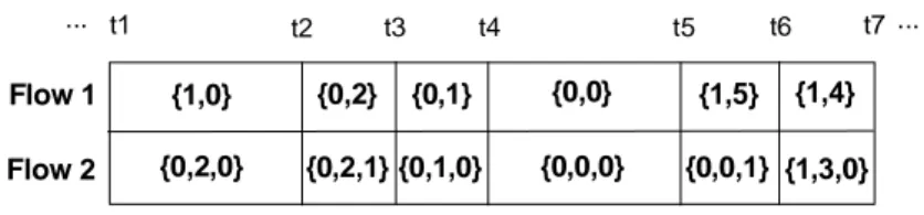
0 . That is to say, for a normal state {s₂(t),b₂(t),0}, the corresponding hold state is further sub-divided into D stages. Therefore, if d(t)>0, the considered traffic flow is waiting at some stage of the hold state. For better understanding the state transitions of different stations carrying different types of traffic, we give an example for the state transitions of two different types of traffic flows in Fig. 2. In the example, for simplicity, we assume that there are only two traffic flows in the system. Flow 1 carries type-1 traffic, and Flow 2 carries type-2 traffic. Moreover, the DIF difference D between inter-frame separation is 1. In the figure, states for the two traffic flows are labeled in the corresponding time slot. In the time slot from t1 to t2, Flow 1 is at state {1,0}, and it begins sending a packet. Flow 2 is at state {0,2,0}. From t2 to t3, after the sending of the packet, Flow 1 begins another backoff process. At the same time, Flow 2 step into the hold state {0,2,1} to wait for the end of DIF2.

From t3 to t4, Flow 1 further decreases its backoff counter from 2 to 1. Flow 2 resumes its backoff process and decreases its backoff counter from 2 to 1. From t4 to t5, both Flow 1

and Flow 2 try to send packets at the same time. Therefore, a collision occurs. From t5 to t6, Flow 1 begins a new backoff process in order to send the packet again. Flow 2 steps into hold state {0,0,1}. From t6 to t7, Flow 2 begins a new backoff process in order to send the collided packet again. Flow 1 continues its backoff process by decreasing its backoff time from 5 to 4.

In the following, we describe the state transitions mathematically:

Case 1: Before packet transmissions (see Fig. 1b)

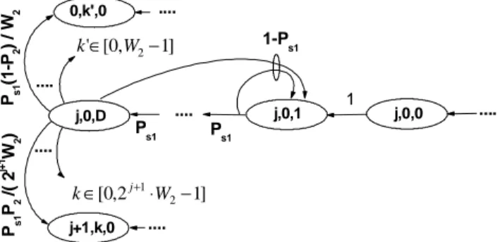
∈ − = + + = + − ∈ = + + + − = + + = + ) 5 . 3 ( ]) , 1 [ ( 1 } , 1 , | 1 , 1 , { ) 4 . 3 ( } , 1 , | 0 , , { ) 3 . 3 ( ]) 1 , 1 [ ( } , 1 , | 1 , 1 , { ) 2 . 3 ( 1 } 0 , 1 , | 1 , 1 , { ) 1 . 3 ( } 0 , 1 , | 0 , , { 1 1 1 D d P d k j k j P P D k j k j P D d P d k j d k j P P k j k j P P k j k j P s s s s s where k [0,2 W2 2],j [0,m2] j⋅ − ∈

∈ . Ps (“probability of silence”) is the probability that all the other traffic flows do not transmit under the condition that the considered traffic flow is at the state of {j,k+1,0}. Note that the considered traffic flow is not at the state of transmission. P_s1

is the probability that all the type-1 traffic flows do not transmit. In order to make the model tractable, we assume that, regardless of the different stages for different hold states, P _s1 is an independent constant probability. This assumption has been shown by our simulation to be very accurate if D is not so large that type-2 traffic flows are almost starved by type-1 traffic flows.

Equation (3.1) accounts for the fact that the backoff counter is decremented at the beginning of each slot time if all traffic flows are not in the state of transmission. Equation (3.2) means that for the considered type-2 traffic flows, if there are some other traffic flows in the state of transmission during the past time slot, its next state is a hold state. If the considered traffic flow is at a hold state, it transits into the next hold state with probability P_s1

(see equation (3.3)). Or it goes back to the first hold state with probability 1−P_s1 because of the transmission of at least one type-1 traffic flow during the past time slot, see equation (3.5). Equation (3.4) shows that for the considered traffic flow, the traffic flow will step into normal state after the last hold state with probability P_s1.

∈ − = − ∈ − ⋅ = − ⋅ ∈ ⋅ ⋅ = − ⋅ ∈ < ⋅ ⋅ = + − ∈ = + = + + ) 6 . 4 ( ]) , 1 [ ( 1 } , 0 , | 1 , 0 , { ) 5 . 4 ( ]) 1 , 0 [ ( ) 1 ( } , 0 , | 0 , , 0 { ) 4 . 4 ( ]) 1 2 , 0 [ ( 2 } , 0 , | 0 , , { ) 3 . 4 ( ]) 1 2 , 0 [ , ( 2 } , 0 , | 0 , , 1 { ) 2 . 4 ( ]) 1 , 1 [ ( } , 0 , | 1 , 0 , { ) 1 . 4 ( 1 } 0 , 0 , | 1 , 0 , { 1 2 2 2 1 2 2 2 1 2 2 2 1 2 2 1 2 1 1 2 2 D d P d j j P W k W p P D j k P W k W p P D m k m P W k m j W p P D j k j P D d P d j d j P j j P s s m m s j j s s

where j∈[0,m₂]. Equation (4.1) accounts for the fact that after the transmission of a packet, the considered type-2 traffic flow steps into hold state with probability 1. If the considered traffic flow is at a hold state, it transits into the next hold state with probability Ps1, see

equation (4.2), or it goes back to the first hold state with probability 1−P_s1 because of the transmission of at least one type-1 traffic flow during the past time slot, see equation (4.6). Equation (4.3) accounts for the fact that a collision occurs and the station carrying type-2 traffic doubles the backoff time after its sending of a packet. Equation (4.4) models the fact that once the backoff stage reaches the value m₂, it is not increased in subsequent packet transmissions. Equation (4.5) accounts for the fact that a new packet following a successful packet transmission starts with backoff stage 0.

From the above descriptions on the state transitions for traffic flows, we can see that with the introduction of the packet collision probabilities p₁ and p₂, hold states for type-2 traffic flows, and probabilities P_s and P_s1, it is possible to solve the Markov chain of a traffic flow independently.

B. Throughput Analysis

First, we solve the Markov chain for type-1 traffic. Let q1(i,j) , i∈[0,m1] and

] 1 2 , 0 [ ₁− ∈ W

j i , be the stationary distribution of the chain. It is easy to find that

⋅ − = < < ⋅ = ) 0 , 0 ( 1 ) 0 , ( ) 0 ( ) 0 , 0 ( ) 0 , ( 1 1 1 1 1 1 1 1 1 1 q p p m q m i q p i q m i (5) and ) 0 , ( 2 2 ) , ( 1 1 1 1 q i W j W j i q _i i ⋅ − = (6)

where i∈[0,m₁] and j∈[0,2iW₁−1]. Because = − = = 1 1 0 1 2 0 1( , ) 1 m i W j i j i q , we have ] ) 2 ( 1 [ ) 1 )( 2 1 ( ) 1 )( 2 1 ( 2 ) 0 , 0 ( 1 1 1 1 1 1 1 1 1 m p W p W p p p q − + + − − − = (7) 1

τ is defined as the probability that a station carrying type-1 traffic transmits in a randomly chosen slot time. We have

] ) 2 ( 1 [ ) 1 )( 2 1 ( ) 2 1 ( 2 ) 0 , ( 1 1 1 1 1 1 1 1 1 1 1 m m i p W pW p p i q − + + − − = = = τ (8)

Please refer to [10] for detailed derivations on equations (5) to (8).

For type-2 traffic, let q₂(i, j,k) , i∈[0,m₂] , j∈[0,2iW₂ −1] and k∈[1,D] , be the stationary distribution of the chain. We derive

⋅ − = < < ⋅ = ) 0 , 0 , 0 ( 1 ) 0 , 0 , ( ) 0 ( ) 0 , 0 , 0 ( ) 0 , 0 , ( 2 2 2 2 2 2 2 2 2 2 q p p m q m i q p i q m i (9) and ) 0 , 0 , ( 2 2 ) 0 , , ( ₂ 2 2 2 q i W j W j i q _i i ⋅ − = (10) where i∈m₂ and j∈[0,2iW₂−1]. Furthermore, it can be easily found that

≤ ≤ = ⋅ ≤ ≤ > − ⋅ = − + − + ) 1 , 0 ( 1 ) 0 , , ( ) 1 , 0 ( ) 1 ( ) 0 , , ( ) , , ( 1 1 2 1 1 2 2 D k j P j i q D k j P P j i q k j i q k D s k D s s (11)

where i∈[0,m₂]. Please refer to the Appendix for the detailed derivations of equations (9) to (11). From above three equations, we can see that all the state probabilities can be expressed by q₂(0,0,0). Because = − = = = 2 2 0 1 2 0 0 2(, , ) 1 m i W j D k i k j i q , we can have: ⋅ − + ⋅ − − − + − − + − + = = = D i i s s m D i i s P P p p p W p W p p P q 1 1 2 2 2 2 2 2 2 2 1 1 2 1 ) 1 ( 1 ) 1 )( 2 1 ( 2 ] ) 2 ( 1 [ ) 1 )( 2 1 ( 1 1 1 1 ) 0 , 0 , 0 ( 2 (12)

Let us define P_hold as the probability that all stations carrying type-2 traffic are in hold states. We emphasize that, if one station carrying type-2 traffic is in hold states, all the other stations carrying type-2 traffic must be in hold states too. P_hold is expressed as

= − = = = 2 2 0 1 2 0 1 2(, , ) m i W j D k hold i k j i q P (13) Moreover, we define τ₂ as the probability that a station carrying type-2 traffic transmits in a randomly chosen slot time under the condition that it is not in hold states. Therefore, we have

] ) 2 ( 1 [ ) 1 )( 2 1 ( ) 2 1 ( 2 ) 0 , , ( ) 0 , 0 , ( 2 2 2 2 2 2 2 2 2 2 0 1 2 0 2 0 2 2 m m i W j m i p W p W p p j i q i q i − + + − − = = = − = = τ (14)

Now we can express P , the probability that all the other traffic flows, except for the _s

considered type-2 traffic flow, are not in the state of transmission, as follows

1 2 1 2 1_{(1 )} ) 1 ( − − − = n n s P τ τ (15) 1 s

P , the probability that all the traffic flows with type-1 are not transmitting, can be given as

1 ) 1 ( ₁ 1 n s P = −τ (16) With the above probabilities defined, we can express the packet collision probabilities p and ₁

2 p as ] ) 1 )( 1 ( [ ) 1 ( 1 1 2 2 1 1 1 n temp temp n P P p = − −τ − + − −τ (17) 1 2 1 2 2 1_{(1 )} ) 1 ( 1 1− = − − − − = n n s P p τ τ (18) Combining equations (8), (11) to (18) and by using SOR numerical method [20], we can get all the values for p , ₁ p , ₂ τ₁, τ₂, P , _s P and _s1 P_hold.

In order to derive the system throughput, we define Q( ji, ) as the probability that there are a number of i type-1 stations and a number of j type-2 stations transmitting within a

randomly selected slot. For Q(0,0), with no transmitting station, we have

] ) 1 )( 1 ( [ ) 1 ( ) 0 , 0 ( 1 2 2 1 n hold hold n P P Q = −τ + − −τ (19) For Q(1,0), with only one type-1 station transmitting, we have

] ) 1 )( 1 ( [ ) 1 ( ) 0 , 1 ( 1 2 2 1 1 1 1 n hold hold n P P n Q = τ −τ − + − −τ (20) For Q(0,1), with only one type-2 station transmitting, we have

1 2 2 2 1 2 1_{(1 ) (1 )} ) 1 ( ) 1 , 0 ( = − n −P_hold n − n − Q τ τ τ (21) For Q(c₁,c₂) (c₁≥2,c₂ =0), which means that there are some collisions occurring between type-1 traffic flows, we have

] ) 1 )( 1 ( [ ) 1 ( ) , ( 1 1 1 2 2 1 1 1 1 2 1 n hold hold c n c P P c n c c Q = τ −τ − ⋅ + − −τ (22) For Q(c₁,c₂) (c₁+c₂ ≥2,c₂ ≥1), we have 2 2 2 1 1 1_{(1 ) (1 ) (1 )} ) , ( _{2 2} 2 2 1 1 1 1 2 1 c n c hold c n c c n P c n c c Q = τ −τ − ⋅ − ⋅ τ −τ − (23) The normalized system throughputs S can be defined and expressed as:

) , ( ) , ( ) 1 , 0 ( ) 0 , 1 ( ) 0 , 0 ( ] [ ) 1 , 0 ( ] [ ) 0 , 1 ( slot time a of length Average slot time a in ed transmitt payload Average 2 1 2 0 0 2 1 2 , 1 , 2 , 1 , 2 1 2 1 2 2 1 1 c c T c c Q T Q T Q Q P E Q P E Q S S S c c c n c n c s s Len Len ⋅ + ⋅ + ⋅ + ⋅ ⋅ + ⋅ = + = ≡ ≥ + ≤ ≤ ≤ ≤ σ (24)

where S and ₁ S denote the throughputs contributed by type-1 and type-2 traffic flows, ₂

respectively. E[PLen,i] is the average duration to transmit the payload for type-i traffic (the

payload size is measured with the time required to transmit it). For simplicity, with the assumption that all packets of type-i traffic have the same fixed size, we have E[PLen,i]=PLen,i.

σ is the duration of an empty time slot. Ts,i (see Fig. 3) is the average time of a slot because of a successful transmission of a packet of a type-i traffic flow. Ts,i can be expressed as

δ δ + + + + + + + = , 1

, PHY MAC E[P ] SIF ACK DIF

Tsi header header Leni (25) where δ is the propagation delay. T_c(c₁,c₂), refer to Fig. 3, is the average time the channel is sensed busy by each station during a collision caused by simultaneous transmissions of c ₁

type-1 stations and c type-2 stations. It can be expressed as ₂

δ θ

θ + +

+ +

=PHY MAC c P c P DIFS

c c

Tc( 1, 2) header header max[ ( 1) Len,1, ( 2) Len,2] (26)

and = > ≡ 0 0 0 1 ) ( x x x θ

C. Packet Delay Analysis

For the quality of service of real-time multimedia it is important to know the time that a packet must wait for transmission over the IEEE 802.11 MAC. By analyzing the packet delay, we can derive an upper bound for the average delay.

For a type-i traffic flow, we define that the whole period of time within T_s,_i (see equation

25) is spent to send a packet. Therefore, for a type-i traffic flow, we define packet delay T_D,i

as the average time period between the instant of its finishing sending the former packets to the instant of beginning to send the next packet. Therefore, T_D,i does not include the transmission time for a packet (see Fig. 4). In Fig. 4, detailed timing relationships between packet sending times and packet delays are illustrated.

Based on Fig. 4, it can be easily found that there is a simple relationship between TD,i and the throughput S : _i i s i D i Len i i i T T P E n S s , , ,] [ + = ≡ (27) Therefore, TD,i for type-i traffic flows can be given as

i s i i Len i D T s P E T _, = [ ,]− _, (28)

IV. Approximate Analysis

In the above two sections, we have analyzed the system throughput and packet delay in saturation state. In order to gain a deeper insight into the whole system, we make some approximations to get simpler but more meaningful relationships among different parameters.

In the following discussion, it is assumed that D=0, that is, we only consider the case that

2

1 DIF

DIF = . We start from equations (17) and (18). BecauseD=0, P_hold must also be 0. Therefore, we can easily derive

∏

It can be seen that if τ1 ≠τ2, then one must have p1≠ p2, which justifies our former

assumption that conditional packet collision probabilities of different types of traffic flows may be different from each other. When the minimum contention window size W1 >>1 andW₂ >>1, the transmission probabilities τ₁ and τ₂ are small, that is, τ₁<<1 andτ₂ <<1. Therefore, from equation (29), we have the following approximation

2

1 p

p ≈ (30) under the condition of W₁ >>1 and W₂ >>1. Furthermore, when W₁ >>1, W₂ >>1 and

2

1 m

m ≈ , we have the following approximation based on equations (8) and (14)

1 2 2 1 W W ≈ ττ (31)

From equations (19), (20) and (24), we have

] [ ] [ ] [ ] [ ] [ ) 1 ( ] [ ) 1 ( ] [ ) 1 , 0 ( ] [ ) 0 , 1 ( 2 , 1 2 1 , 2 1 2 , 2 2 1 , 1 1 2 , 1 2 2 1 , 2 1 1 2 , 1 , 2 1 Len Len Len Len Len Len Len Len P E W n P E W n P E n P E n P E n P E n P E Q P E Q S S ≈ ≈ − − = ⋅ ⋅ = τ τ τ τ τ τ (32) Then, from the above equation, we have

2 2 , 1 1 , 2 1 ] [ ] [ W P E W P E s s Len Len ≈ (33)

The above equation holds under the conditions of D=0, W₁ >>1 and W₂ >>1 and m₁≈m₂. We can see that the throughput differentiation is mainly determined by the scaling of minimum contention window sizes and the length of packet payloads.

Moreover, from equation (28), we can see that under the condition

i i Len i s s P E T_, << [ ,] ) 2 , 1

(i= , which always holds when the number of traffic flows n_i >>1 (i =1,2), we have

2 1 2 2 , 1 1 , 2 , 1 , ] [ ] [ W W s P E s P E T T Len Len D D ≈ ≈ (34)

Equation (34) is another important approximation relationship obtained. We can see that packet delay differentiation among different types of traffic flows is mainly determined by the ratio of the corresponding minimum contention window sizes.

Assuming that all the W and _i E[PLen,i] are fixed, then from equations (33), (34), and (28)

we can easily arrive at the following conclusions:

1. s can be linearly expressed by 2 s , that is, 1 1

1 , 2 2 , 1 2 ] [ ] [ s P E W P E W s Len Len _⋅

≈ . Therefore, s reaches its 2

maximum value when s reaches its maximum value. That is to say, there is a case where ₁

all throughputs s_i(i=1,2) and the total throughput S of the system reach their maximum values at almost the same configuration.

2. TD,2 can be linearly expressed by TD,1, that is, ,1 1 2 2 , D D T W W

minimum value when T_D,1 reaches its minimum value. That is to say, there is a case where all the packet delays T_D,i(i=1,2) reach their minimum values at almost the same configuration.

3. When all throughputs s_i(i=1,2) reach their maximum value, all the T_D,i will reach their minimum values at almost the same configuration.

The above properties show that by scaling W and _i E[PLen,i] one can obtain service

differentiation and make the whole system easily controllable.

V. Results And Discussions

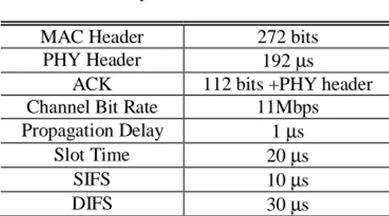
In this section, by using our analysis model we investigate the effect of the different parameters on the traffic differentiation and we validate the analysis assumptions by comparisons with a discrete-event simulation of the system. In addition, we assess the range of validity of the approximated formulas obtained in the previous analysis. We proceed by first considering the effect of varying a single crucial parameter on the performance differentiation and then by considering the validity of the approximated formulas for the case of equal inter-frame separations. In our examples, we assume that two types of traffic coexist in the system. The parameters for the system are summarized in Table 1 based on IEEE 802.11b.

The purpose of the first series of experiments is to verify the accuracy of our analysis model and assess the effect of varying the inter-frame separations on the performance. To this end, we keep all other parameters equal and only change the value of D. In Fig. 5 and Fig. 6, we validate our proposed analysis model by comparing simulation results and numerical results. For our simulator, which is implemented by using C++, we consider that there are 20

Table 1. System Parameters

MAC Header 272 bits PHY Header 192 µs

ACK 112 bits +PHY header Channel Bit Rate 11Mbps Propagation Delay 1 µs

Slot Time 20 µs

SIFS 10 µs

stations each carrying only one traffic flow. 5 of them carry type-1 traffic and the others carry type-2 traffic. In the simulation, ideal channel conditions (i.e., no hidden terminals and capture) are assumed. The other parameters are set as follows: W₁=W₂ =64, m₁=m₂ =8 and

bytes P

E P

E[ _Len,1]= [ _Len,2]=2000 . Different simulation values are obtained by varying the IFS difference D. Each simulation values are obtained by running our discrete-event simulator to simulate the actual behavior of the system within the period of 5 hours. For each point, we run the simulator for 10 times with 10 different random seeds. Simulation results show that the standard deviation of the results caused by using different random seeds is less then one percent for each point, and therefore not visible in the figures.

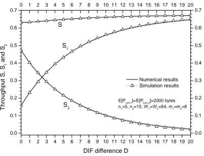
In Fig. 5, throughput S, S and ₁ S versus IFS difference ₂ D are shown. In Fig. 6, average packet delays TD,1 , TD,2 and the overall average packet delay per traffic flow

2 1 2 , 2 1 , 1 n n T n T n T_D D D + +

≡ are shown versus the IFS difference D. From these two figures, it can be seen that the simulation results agree very well with the theoretical ones. We can also see that the smaller D, the better the simulation results agree with the numerical ones, which suggests that the accuracy of our assumption of the probability P being a constant is accurate and _s1

reasonable for this case. On the other hand, when D increases, the difference between simulation results and numerical ones becomes more evident. In order to understand the reason, let us consider an extreme case, where the maximum contention window size CW_max

for type-1 traffic is smaller thanD. It is evident that, in this case, after the period of transmission of a packet or collision between some packets, it is entirely impossible for type-2 traffic flows to get access to the channel. In this case, the backoff process for type-2 traffic flows will not proceed from one normal state to another. However, by referring to Fig. 1b and equations (15) and (16), it can be found that in most cases, one can always get positive and nonzero P and _s1 P , which means that the backoff process of type-2 traffic flows will always _s

go on, and type-2 traffic flows will eventually access the channel even in the above extreme case. Therefore, our model is only an approximation, needed to make our model tractable. Moreover, extensive simulations show that our model is very accurate as long as type-2 traffic flows are not heavily starved by type-1 traffic. From these two figures, we can quantify the differentiating effects caused byD. With the increase of D, more channel resources are allocated to type-1 traffic flows, and also the average packet transmission delay for type-1 traffic decreases. When D becomes larger, the rate for the performance improvement of

type-1 traffic decreases, and at the same time, performance for type-2 traffic becomes worse, which indicates that a very large D is not much helpful to improve the system performance.

The purpose of the second series of experiments for the case D=0 is to verify the range of validity of the approximated formulas derived in the paper. In the experiments, two cases have been shown. In case 1, we set E[PLen,1]=E[PLen,2]=2000bytes. In case 2, different packet

payloads for two types of traffic have been set, i.e., E[PLen,1]=2000bytes and bytes

P

E[ Len,2]=200 . Other parameters are set as follows: W2 =256 , m1=m2 =2 ,

25

2

1=n =

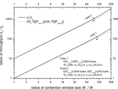
n . Fig. 7 and Fig. 8 show a comparison between throughput and packet delays obtained by using accurate theoretical formulas and those obtained by using approximate formulas. In Fig. 7, the values of

2 1 s s

are compared with those of

] [ ] [ 2 , 1 1 , 2 Len Len P E W P E W ⋅ ⋅ . We can see that when 1 2 W W

is not large, that is, W is not very small, the ratio ₁ 2 1 s s can be approximated by ] [ ] [ 2 , 1 1 , 2 Len Len P E W P E W ⋅ ⋅

fairly well, which verifies our approximation made in equation (33). Furthermore, we can verify that the length of the packet payload has an immediate effect on the throughput differentiation between different traffic classes. In Fig. 8, the values of

1 , 2 , D D T T

are compared with those of

1 2 W W

. Again, we can see that when

1 2 W W

is not large, the ratio

1 , 2 , D D T T can be approximated by 1 2 W W

fairly well, which verifies our approximation made in equation

(34). Moreover, we notice that the corresponding values of

1 , 2 , D D T T

for two different cases are overlapped (the maximum differences between these two cases are less then one percent), which indicates that packet payload almost has no influence on the values of

1 , 2 , D D T T . That is to say, scaling the length of packet payload has little effect on the differentiation of packet delays between the different traffic classes.

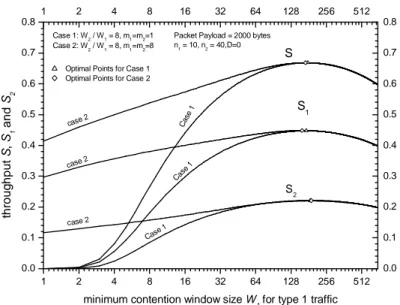
Let us now consider the optimization of the overall performance of the system. In the former section, in the case of D=0, and by using the approximated formulas, we point out that there is a case where all throughputs s and the total throughput _i S of the system reach

their maximum values at almost the same configuration. And we also point out that there is a case where all packet delays T_D,_i reach their minimum values at almost the same time. In Fig.

9 and Fig. 10, these conclusions are verified by using numerical results. In these figures, we keep the ratio

1 2 W W

constant and change the value W , in order to see the variations of 1

throughput and packet delays of different types of traffic. In these two figures, two cases have been shown. Moreover, maximum throughput points and minimum packet delay points are shown. From Fig.9, we can see that for a particular case S, si(i=1,2) reaches their maximum values almost at the same W , which verifies our first conclusion made in the former section. ₁

And from Fig. 10, we can see that for a particular case TD,i(i=1,2) reaches their maximum

values almost at the sameW , which verifies our second conclusion made in the former 1

section. Moreover, by checking these two figures together, we can find that si(i=1,2) and corresponding TD,i(i=1,2) reach their optimal points at exactly the same W , which in turn 1

justifies our third conclusion made in the former section. From these two figures, by comparing case 1 and case 2, we find that, as expected, the system becomes more stable with the increase of maximum backoff stages m and ₁ m . This is because that with larger ₂ m and ₁

2

m packet collision rates drop, which increases the utilization of the whole system.

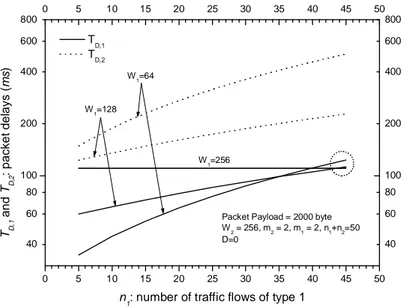
Let us now consider the effect of the “traffic mixture” on the performance. To this end we fix the total number of flows and vary the relative portion of high- versus low-priority flows. In Fig. 11 and Fig. 12, we keep the total number of traffic flows constant, and change the number n of type-1 traffic flows in the case of ₁ D=0. In Fig. 11, throughputs s and ₁ s ₂

versus the number of type-1 traffic flows n are shown. Different curves are for different ₁

values of the minimum contention window size W . In Fig. 12, the packet delays ₁ TD,1 and 2

,

D

T for two types of traffic are shown in the same configuration. From Fig. 11 and Fig. 12, we can see that with the decrease of W , type-1 traffic flows gain priority over type-2 traffic ₁

flows: throughput s becomes larger than ₁ s , and packet delay ₂ TD,1 becomes smaller than 2

,

D

T . Therefore, more bandwidth resources are allocated to type-1 traffic. However, we can see that in the case of large n (such as 1 n1>40), both the performance on throughput and

packet delays are worse than in the case of W₁=W₂ =256, which indicates that providing service differentiation with very large number of traffic flows belonging to higher priority

group makes the system performance worse than in the case of no service differentiation support. In this case, performance of all traffic flows, no matter if they belong to higher or lower priority classes, becomes worse.

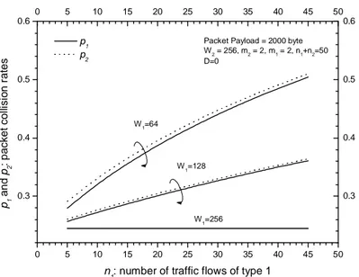
The reason can be easily explained by referring to Fig. 13, that shows the packet collision rates p and 1 p for two types of traffic. We can see that with the increase of 2 n , collision 1

rates p and ₁ p increase drastically, therefore reducing the bandwidth utilization. On the ₂

other hand, from Fig. 13, it can be seen that with the increase of W , the difference between ₁ 1

p and p decreases, in agreement with the approximation obtained in equation (30). ₂

Moreover, referring to Fig. 11 and Fig. 12, if the number of traffic flows with higher priority is small, both throughput and packet delays for higher priority traffic flows are improved significantly with only small influence on the other traffic flows with lower priority. The above results indicate that the number of traffic flows with higher priority must be controlled to a suitable fraction of the total traffic by suitable access control schemes.

Finally, when one considers implementing some real system to support service differentiation, simplicity should also be considered. It is always the case that the simpler the scheme is, the lower the system costs. In our model, three service differentiation supporting mechanisms are analyzed. By adopting the scheme of differentiating minimum contention window sizes and packet payloads of different traffic types, simple relationships exist among throughput and packet delays, which is helpful to simplify the design of the whole system. On the other hand, in order to make the system as simple as possible, one should limit the number of parameters that can be adjusted. On the whole, by using the analysis model proposed in this paper, we can obtain deeper insight, which is important and helpful to the design of real systems. However, the implementation issues of real systems are beyond the scope of this paper, although they are very important research topics for our future work.

VI. Conclusions

We proposed an analysis model to compute the throughput and packet transmission delays in a WLAN with enhanced IEEE 802.11 Distributed Coordination Function, which supports service differentiation. In our analytical model, service differentiation is supported by scaling the contention window, the Inter-Frame Spacing (IFS) and the packet length according to the priority of each traffic flow. Comparisons with simulation results show that good accuracy of performance evaluations can be achieved by using the proposed model.

In particular, we evaluated the throughput and packet delay. It is shown that:

1. The settings of CW_min for different types of traffic flows have significant influence on the throughput and packet delay. One type of traffic gains priority over other types of traffic through a smaller minimum contention window size. More channel resources are occupied, with a smaller packet delay.

2. Traffic flows with shorter IFS obtain higher priority to access to the channel resources. However, excessive IFS values cause very long packet delays for traffic flows with lower priority, bordering on starvation.

3. The length of packet payload of different types of traffic directly influences the bandwidth allocation among different types of traffic flows. However, the differentiation of packet payload size has little influence on the differentiation of packet delays. Let us note that in noisy channel conditions, the typical situation in wireless LANs, longer payloads suffer a higher error probability and this fact may discourage applying payload length variability as a differentiation mechanism.

4. The number of traffic flows with higher priority must be limited to maintain the system working at a high performance regime by suitable access control or pricing schemes. See, for example, [21] for a possible adaptive scheme to regulate the appropriate number of transmitting stations.

5. By adopting the scheme of scaling minimum contention window sizes and packet payloads, approximate and simple relationships exist among throughput, packet delays and lengths of packet payload of different traffic types, which can be used for the optimal design of the whole system.

By using the proposed model, three different service differentiation schemes have been analyzed. The schemes are not mutually exclusive. The appropriate choice and setting of parameters for the control of a real-world system, including access control, is an interesting area of future research that can be benefit from the analysis presented in this paper.

References

[1] Y. Cheng and W. H. Zhuang, “DiffServ resource allocation for fast handoff in wireless mobile Internet,” IEEE Communications Magazine, vol. 40, no. 5, 2002, pp. 130-136.

[2] R. Braden, D. Clark and S. Shenker, “Integrated services in the Internet architecture: an overview,” IETF RFC 1633, Jun. 1994.

services,” IETF RFC 2475, Dec. 1998.

[4] Wireless LAN Medium Access Control (MAC) and Physical Layer (PHY) specifications, IEEE Standard 802.11, Aug. 1999.

[5] J. Weinmiller, M. Schlager, A. Festag, and A. Wolisz, “Performance study of access control in wireless LANs IEEE 802.11 DFWMAC and ETSI RES 10 HIPERLAN,” Mobile Networks and Applications, vol. 2, pp. 55-67, 1997.

[6] H. S. Chhaya and S. Gupta, “Performance modeling of asynchronous data transfer methods of IEEE 802.11 MAC protocol,” Wireless Networks, vol. 3, pp. 217-234, 1997.

[7] T. S. Ho and K. C. Chen, “Performance evaluation and enhancement of the CSMA/CA MAC protocol for 802.11 wireless LAN’s,” Proceedings of IEEE PIMRC, Taipei, Taiwan, Oct. 1996, pp.392-396.

[8] F. Cali, M. Conti, and E. Gregori, “IEEE 802.11 wireless LAN: Capacity analysis and protocol enhancement,” Proceedings of INFOCOM’98, San Francisco, CA, March 1998, vol. 1, pp. 142 -149.

[9] G. Bianchi, L. Fratta, and M. Oliveri, “Performance analysis of IEEE 802.11 CSMA/CA medium access control protocol,” Proceedings of IEEE PIMRC, Taipei, Taiwan, Oct. 1996, pp. 407-411.

[10] G. Bianchi, “Performance analysis of the IEEE 802.11 distributed coordination function,” IEEE Journal on Selected Areas In Communications, vol. 18, no. 3, March 2000.

[11] Y. C. Tay and K. C. Chua, “A Capacity Analysis for the IEEE 802.11 MAC Protocol,” Wireless Networks, 7, 2001, pp. 159-171.

[12] J. L. Sobrinho and A. S. Krishnakumar, “Distributed multiple access procedures to provide voice communications over IEEE 802.11 wireless networks,” Proceedings GLOBECOM 1996, pp. 1689-1694. [13] J. Deng and R.S. Chang, “A priority scheme for IEEE 802.11 DCF access method,” IEICE Transactions

in Communications, vol. 82-B, no. 1, Jan 1999, pp. 96-102.

[14] A. Veres, A. T. Campbell, M. Barry and L. H. Sun, “Supporting Service Differentiation in Wirelss Packet Networks Using Distributed Control,” IEEE Journal on Selected Areas In Communications, vol. 19, no. 10, Oct 2001, pp. 2081-2093.

[15] I. Aad and C. Castelluccia, “Differentiation Mechanisms for IEEE 802.11,” Proceedings of IEEE Inforcom 2001, pp. 209-218.

[16] W. Haitao, C. Shiduan, P. Yong, L. Keping, and M. Jian, “IEEE 802.11 distributed coordination function (DCF): analysis and enhancement,” Proceedings of ICC 2002, pp. 605-609.

[17] S. Mangold, S. Choi, P. May, O. Klein, G. Hietz and L. Stibor, “IEEE 802.11e wireless lan for quality of service,” Proceedings of the European Wireless, Feb 2002.

[18] M. Benveniste, G. Chesson, M. Hoehen, A. Singla, H. Teunissen, and M.Wentink, “EDCF proposed draft text,” IEEE working document 802.11-01/131r1, March 2001.

[19] A. Lindgren, A. Almquist, and O. Schelen, “Evaluation of quality of service schemes for IEEE 802.11 wireless LANs,” Proceedings of IEEE Conference on Local Computer Networks (LCN 2001), November 15-16, 2001, pp. 348 –351.

[20] G. Bolch, S. Greiner, H. de Meer, and K.S. Trivedi, Queueing Networks and Markov Chains: Modeling and Performance Evaluation with Computer Science Applications, Wiley-Interscience, 1998, pp. 140-144. [21] Roberto Battiti, Marco Conti, Enrico Gregori, Mikalai Sabel, “Price-based Congestion-Control in Wi-Fi Hot

Appendix: Derivations on Equations (9), (10) and (11)

From Fig. 1b, for i∈[0,m2],0< j≤2W2 −1 i , we have − ⋅ + ⋅ − = ⋅ − + ⋅ − = ⋅ − + ⋅ − = ≤ < − ⋅ = − = = ) 1 ( ) 1 , , ( ) 0 , , ( ) 1 ( ) 1 , , ( ) 1 ( ) 0 , , ( ) 1 ( ) , , ( ) 1 ( ) 0 , , ( ) 1 ( ) 1 , , ( ) 1 ( ) 1 , , ( ) , , ( 1 2 2 1 0 1 2 1 2 1 2 1 2 2 2 1 2 D s s D k k s s s D k s s s P j i q j i q P P j i q P j i q P k j i q P j i q P j i q D k k j i q P k j i q (A.1)

From above equation, we have

) 1 , 1 2 0 ], , 0 [ ( ) 0 , , ( 1 ) , , ( _{1 2 2 2} 1 2 q i j i m j W k D P P k j i q _{D k} i s s ⋅ ∈ < ≤ − ≤ ≤ − = ₊₋ (A.2)

Moreover, for the case of i∈[0,m₂],j=0, we have

− ⋅ + = ⋅ − + = ⋅ − + = ≤ < − ⋅ = − = = ) 1 ( ) 1 , 0 , ( ) 0 , 0 , ( ) 1 , 0 , ( ) 1 ( ) 0 , 0 , ( ) , 0 , ( ) 1 ( ) 0 , 0 , ( ) 1 , 0 , ( ) 1 ( ) 1 , 0 , ( ) , 0 , ( 1 2 2 1 0 1 2 1 2 1 2 1 2 2 2 1 2 D s D k k s s D k s s P i q i q P i q P i q k i q P i q i q D k k i q P k i q (A.3) then, ) 1 ], , 0 [ ( ) 0 , 0 , ( 1 ) , 0 , ( _{1 2 2} 1 2 q i i m k D P k i q _{D k} s ≤ ≤ ∈ ⋅ = ₊₋ (A.4) By combining equations (A.2) and (A.4), equation (11) can be obtained.

Next, we subdivided our discussions into three different cases:

Case 1: when 0<i<m2

From the description on the Markov chain for type 2 traffic flows, we have

− ≤ ≤ ⋅ − + + = ⋅ ⋅ − + + ⋅ + + ⋅ = ⋅ − = ⋅ ⋅ − = − ) 2 2 0 ( 2 ) 0 , 0 , 1 ( ) 0 , 1 , ( 2 ) , 0 , 1 ( ) , 1 , ( ) 0 , 1 , ( ) 0 , , ( 2 ) 0 , 0 , 1 ( 2 ) , 0 , 1 ( ) 0 , 1 2 , ( 2 2 2 2 2 2 2 1 2 2 1 2 2 2 2 2 2 2 1 2 2 2 W j W p i q j i q W p P D i q D j i q P j i q P j i q W p i q W p P D i q W i q i i i s s s i i s i (A.5)

) 1 2 0 ( ) 0 , 0 , 1 ( 2 2 ) 0 , , ( _{2 2 2} 2 2 2 ⋅ ⋅ − ≤ ≤ − − = p q i j W W j W j i q _i i i (A.6) In equation (A.6), let j=0, one derives

) 0 , 0 , 1 ( ) 0 , 0 , ( _{2 2} 2 i = p ⋅q i− q (A.7) and then ) 1 2 0 ( ) 0 , 0 , ( 2 2 ) 0 , , ( 2 2 2 2 2 ⋅ ≤ ≤ − − = q i j W W j W j i q _i i i (A.8) Case 2: when i=m₂ We have − ≤ ≤ ⋅ + − + + = ⋅ ⋅ + ⋅ ⋅ − + + ⋅ + + ⋅ = ⋅ + − = ⋅ ⋅ + ⋅ ⋅ − = − ) 2 2 0 ( 2 )] 0 , 0 , ( ) 0 , 0 , 1 ( [ ) 0 , 1 , ( 2 ) , 0 , ( 2 ) , 0 , 1 ( ) , 1 , ( ) 0 , 1 , ( ) 0 , , ( 2 )] 0 , 0 , ( ) 0 , 0 , 1 ( [ 2 ) , 0 , ( 2 ) , 0 , 1 ( ) 0 , 1 2 , ( 2 2 2 2 2 2 2 2 2 2 2 1 2 2 2 2 1 2 2 2 2 1 2 2 2 2 2 2 2 2 2 2 2 2 1 2 2 2 2 1 2 2 2 2 2 2 2 2 2 2 2 2 2 W j W p m q m q j m q W p P D m q W p P D m q D j m q P j m q P j m q W p m q m q W p P D m q W p P D m q W m q m m m s m s s s m m s m s m (A.9)

From equation (A.9), we have

) 1 2 0 ( )] 0 , 0 , ( ) 0 , 0 , 1 ( [ 2 2 ) 0 , , ( 2 2 2 2 2 2 2 2 2 2 2 2 2 − ≤ ≤ + − ⋅ ⋅ − = p q m q m j W W j W j m q _m m m (A.10) By setting j=0, from above equation and equation (A.7), we have

) 0 , 0 , 0 ( 1 ) 0 , 0 , ( ₂ 2 2 2 2 2 q p p m q m ⋅ − = (A.11) Combining equations (A.7) and (A.11), we can obtain equation (9). Moreover, we have

) 1 2 0 ( ) 0 , 0 , ( 2 2 ) 0 , , ( 2 2 2 2 2 2 2 2 2 2 − ≤ ≤ ⋅ − = q m j W W j W j m q _m m m (A.12) Case 3: i=0

− ≤ ≤ ⋅ − + + = ⋅ − ⋅ + + ⋅ + + ⋅ = ⋅ − = ⋅ − ⋅ = − = = = = ) 2 0 ( ) 0 , 0 , ( ) 1 ( ) 0 , 1 , 0 ( ) , 0 , ( ) 1 ( ) , 1 , 0 ( ) 0 , 1 , 0 ( ) 0 , , 0 ( ) 0 , 0 , ( ) 1 ( ) , 0 , ( ) 1 ( ) 0 , 1 , 0 ( 2 0 2 2 2 2 0 2 2 2 1 2 1 2 2 0 2 2 2 0 2 2 2 1 2 2 2 2 2 2 W j i q W p j q D i q W p P D j q P j q P j q i q W p D i q W p P W q m i m i s s s m i m i s (A.13) then, 1) -(0 ) 0 , 0 , ( ) 1 ( ) 0 , , 0 ( 2 0 2 2 2 2 2 2 W j i q p W j W j q m i ≤ ≤ ⋅ − ⋅ − = = (A.14) From equation (9), the above equation can be reduced into the following equation

1) -(0 ) 0 , 0 , 0 ( ) 0 , , 0 ( _{2 2} 2 2 2 q j W W j W j q = − ⋅ ≤ ≤ (A.15) From equations (A.8), (A.12) and (A.15), we can obtain equation (10).

Fig. 1a Markov model of backoff process for type 1 traffic

Fig. 1b Transitions out of state {j,k+1,0} for type 2 traffic

Fig. 1c Transitions out of state {j,0,0} for type 2 traffic

1 1 1 1 1 1 1 1 1 1 1 1 1 1 p₁/(2j+1 W₁) ... ... ... ... ... ... ... ... ... p₁/(2m1 _W 1) p₁/(2m1 _W 1) p₁/(2j W₁) p₁/(21 W₁) (1-p₁) / W₁ 0,W₁-1 0,W 1-2 0,1 0,0 j-1,1 j-1,0 j,2j W₁-1 j,2j W 1-2 j,1 j,0 m 1,0 m1,1 m1,2 m1 _W 1-2 m1,2 m1 _W 1-1 .... .... .... j,k+1,D j,k+1,D-1 j,k+1,1 j,k,0 j,k+1,0 P_s1 Ps1 1-P s1 P_s1 1-P_s P s .... .... Ps 1 P2 / ( 2 j+ 1 W 2 ) Ps 1 (1 -P2 ) / W2 ] 1 2 , 0 [ 1_{⋅ 2−} ∈ + _W k j ] 1 , 0 [ '∈ W₂− k .... .... j,0,D .... j,0,1 1 .... 0,k',0 j+1,k,0 j,0,0 P s1 1-P s1 P_s1

Fig. 2 An example for state transitions of two different type of traffic flows

Fig. 3 Components for T_s,_i and Tc(c1,c2)

Fig. 4 Analysis of the packet delay

Note:

Flow 1: Carrying type 1 traffic with W

1=8, m1=2

Flow 2: Carrying type 2 traffic with W₂=8, m₂=2

D=1 Flow 2 Flow 1 ... ... _{t1 t2 t3 t4 t5 t6 t7} {1,3,0} {1,4} {1,5} {0,0,1} {0,0,0} {0,0} {0,1} {0,1,0} {0,2,1} {0,2} {0,2,0} {1,0} T c(c1,c2) Payload Header DIF₁ T_s,i

SIF ACK DIF₁

Payload Header T_D,1=Delay T_D,2=Delay₁+Delay₂ Delay₂ Type 2 traffic Start Backoff for the next packet

... Hold States Start Backoff

for the current packet

Delay₁ Header Payload SIF ACK DIF1

Delay

... Start Backoff for the next packet Start Backoff

for the current packet

Type 1 traffic

SIF ACK DIF₁

Payload Header

Fig. 5 Throughput S, S₁ and S₂ versus D

Fig. 6 Average packet delays T_D,1, T_D,2 and T_D versus D

0 1 2 3 4 5 6 7 8 9 10 11 12 13 14 15 16 17 18 19 20 0.0 0.1 0.2 0.3 0.4 0.5 0.6 0.7 0 1 2 3 4 5 6 7 8 9 10 11 12 13 14 15 16 17 18 19 20 0.0 0.1 0.2 0.3 0.4 0.5 0.6 0.7

S₂ E[PLen,1]=E[PLen,2]=2000 bytes

n1=5, n2=15, W1=W2=64, m1=m2=8 S₁ S T h ro u g h p u t S , S1 a n d S 2 DIF difference D Numerical results Simulation results 0 1 2 3 4 5 6 7 8 9 10 11 12 13 14 15 16 17 18 19 20 10 100 1000 0 1 2 3 4 5 6 7 8 9 10 11 12 13 14 15 16 17 18 19 20 10 100 1000 T D

E[P_Len,1]=E[P_Len,2]=2000 bytes

n₁=5, n₂=15, W₁=W₂=64, m₁=m₂=8 T_D,2 T_D,1 A v e ra g e P a c k e t D e la y s ( m s ) DIF difference D Numerical results Simulation results

Fig. 7 Ratios of throughput s₁/ s₂ versus ratios of contention window size W₂ /W₁

Fig. 8 Ratios of packet delay TD_,2/TD_,1 versus ratios of contention window size W2 /W1

1 2 4 8 16 32 64 128 256 1 10 100 1000 1 2 4 8 16 32 64 128 256 1 10 100 1000 ra ti o s o f th ro u g h p u t s1 / s2 case 1 Case 1: E[P

Len,1]=E[PLen,2]=2000 bytes

W₂=256, m₁=m₂=2, n₁=n₂=25,D=0 Case 2:

E[P_Len,1]=2000 bytes, E[P_Len,2]=200 bytes W₂=256, m₁=m₂=2, n₁=n₂=25,D=0

case

2

ratios of contention window size W₂ / W₁

s₁/s₂

(W₂*E[P_Len,1])/(W₁*E[P_Len,2])

1 2 4 8 16 32 64 128 256 1 10 100 1000 1 2 4 8 16 32 64 128 256 1 10 100 1000 r a ti o s o f p a c k e t d e la y TD ,2 / TD ,1 case 1 Case 1:

E[PLen,1]=E[PLen,2]=2000 bytes

W2=256, m1=m2=2, n1=n2=25,D=0

Case 2:

E[P_Len,1]=2000 bytes, E[P_Len,1]=200 bytes W₂=256, m₁=m₂=2, n₁=n₂=25,D=0

case

2

ratios of contention window size W₂ / W₁

T

D,2 / TD,1

W

1 2 4 8 16 32 64 128 256 512 0.0 0.1 0.2 0.3 0.4 0.5 0.6 0.7 0.8 1 2 4 8 16 32 64 128 256 512 0.0 0.1 0.2 0.3 0.4 0.5 0.6 0.7 0.8 case 2 case 2 Cas e 1 Case 1 Ca se 1 case 2

Optimal Points for Case 1 Optimal Points for Case 2 Case 1: W2 / W1 = 8, m1=m2=1 Case 2: W2 / W1 = 8, m1=m2=8 S 1 S₂ S Packet Payload = 2000 bytes n 1 = 10, n2 = 40,D=0 th ro u g h p u t S , S1 a n d S 2

minimum contention window size W

1 for type 1 traffic

Fig. 9 Throughput S, S₁ and S₂versus contention window size W₁

1 2 4 8 16 32 64 128 256 512 100 1000 1 2 4 8 16 32 64 128 256 512 100 1000 Case 2 Case 2 C a_s e 1 C as

e 1 Optimal Points for Case 1

Optimal Points for Case 2

T_D,1 T D,2 Case 1: W2 / W1 = 8, m1=m2=1 Case 2: W 2 / W1 = 8, m1=m2=8

Packet Payload = 2000 bytes n1 = 10, n2 = 40,D=0 p a c k e t d e la y TD ,1 a n d TD ,2 ( m s )

minimum contention window size W

1 for type 1 traffic