Acknowledgement
This Master thesis was accomplished within the Erasmus Mundus Joint Master Degree “Photonic Integrated
Circuits, Sensors and NETworks (PIXNET)”.
Coordinating Institution: Scuola Superiore di Studi Universitari e di Perfezionamento Sant'anna
Partners
Osaka University
Aston University
Technische Universiteit Eindhoven
Project Data
Start: 01-09-2017 - End: 31-08-2022
Project Reference: 586665-EPP-1-2017-1-IT-EPPKA1-JMD-MOB
EU Grant: 3.334.000 EUR
Website: http://pixnet.santannapisa.it
Programme: Erasmus+
Key Action: Learning Mobility of Individuals
Abstract— This project works on characterization of an AWG sample and analysis of the data obtained from this and several other measurements by using python programs. The analysis also compares the parameters of an AWG using data obtained among the different measurements taken as well as with the simulation data. Two sets of measurement data are analyzed, with one set taken in the lab using the measurement setup described in this work and the other set measured by someone else.
Index Terms—array waveguide gratings, spectrometers, wavelength filters, sensors
I. INTRODUCTION
Arrayed waveguide gratings (AWGs) are essential components in wavelength division multiplexed (WDM) communication networks. They have many applications in telecommunications most of which are rooted from their use as wavelength multiplexers and demultiplexers. They can be used to make add and drop multiplexers, tunable wavelength lasers, multi-wavelength receivers, channel selectors and equalizers, sensors, spectrometers and multi-wavelength filters [1]. This work consists of two parts, one involving the collection of data in the lab and analyzing the data obtained and the other will only analyze the data measured by someone else. The first part will focus on characterization an AWG sample where five measurements are taken to test the stability of the measurement setup. The ultimate purpose of the first part is to come up with a stable and fully automatic measurement setup as well as automatic data analysis procedures to be used in characterization and data analysis of several other AWG samples easily. The AWGs to be characterized in the first part are meant to be used as sensors [2], spectrometers [3] and wavelength filters for aerospace applications. The second part will be an application of the data analysis procedures to analyze a data set of 6 types of AWGs each type with 28 AWG samples. The data analysis is done by using python programs developed as a part of this work. This paper is therefore organized in eight sections as follows.
A brief discussion of the working principle of an AWG [4] and technology platforms over which AWGs are made will be in the next section. The third section will discuss the applications of AWGs as sensors, wavelength filters and spectrometers with some specific examples. The fourth section will give a detailed explanation of the parameters of an AWG giving an insight of how the python programs were developed. The fifth section will talk about part one of this work discussing the measurement setup, how the measurements are taken in the lab followed a discussion of experimental and data analysis results as well as the suggested improved setup. The sixth section will describe the second part of this work which involves data analysis of 6 different types of AWGs with 28 samples for each type. The automation and the main analysis steps will be in the seventh section and the last section will conclude this work.
II. THE WORKING PRINCIPLE AND TECHNOLOGY PLATFORMS
Characterization and data analysis of AWGs
used for Sensor PICs, spectrometers and
wavelength filters for aerospace sensing
Balthazar Gaspar Temu
Electrical and Electronics Engineering Department, Technische Universiteit Eindhoven (Collaboration with Bright Photonics)
Eindhoven, Netherlands
[email protected]
Fig 1. Main parts of an array waguide gratings.
The working principle of an AWG:
The AWG has five sections as shown above (written below in bold). The optical signal enters through the transmitter waveguide which leads it into the input free propagation region (FPR). When the light reaches the input FPR it is not guided anymore but becomes divergent. When the signal reaches the input aperture it enters the array waveguides propagates through the array waveguides to the output aperture. The array waveguides are designed in such a way that the optical path length difference between any two adjacent waveguides is an integer multiple of the central wavelength in the waveguides. On reaching the output aperture the optical signal enters the output free propagation region. The effect of linearly increasing the length of the array waveguides leads to a wavelength dependent phase shift (as shown by equation 1) which in turn appears as a wavelength dependent tilt which causes the spatial separation of the different wavelength at the image plane. The receiver waveguides are then placed at the proper location along the image plane so that the different wavelengths propagate out through these output waveguides.
Δφ =
2π λn ΔL
(1)From equation 1 above it is clear that the phase change Δφ is dependent on wavelength λ, refractive index n and length increment ΔL.
AWGs Technology platforms:
AWGs have been realized using different technologies as described below.
Silica-on-silicon (SoS ) waveguides have low index contrast, hence large bending radius which implies the AWGs are big in size
and thus only low integration density on a chip is possible. Their waveguide’s modal field matches well with that of a single mode fiber, and therefore it is relatively easy to couple them to single mode fibers. They have low propagation loss.
Indiumphosphide (InP) waveguides have large index-contrast and hence small bending radius which implies the AWGs are small
(compact) in size and thus can have high integration density on a chip. They have high coupling losses to single-mode fibers. They can be monolithically integrated with active devices like lasers, semiconductor optical amplifiers (SOA), RF-modulators and switches, wavelength converters, signal regenerators or detectors. Insertion-losses of InP and silica AWGs are comparable.
Silicon on Insulator and silicon nanowire waveguides have high refractive index difference between the Si core and the SiO2
cladding which allows small bending radius and hence compact devices. The high index contrast of silicon-on-insulator (SOI) also makes it possible to achieve AWGs with high spectral resolution and channel density. Ultra-compact AWGs can be manufactured using silicon wire technology . The silicon nanowire technology requires very high resolution fabrication technology and usually its devices have high insertion loss and high crosstalk.
Silicon Nitride technology is the platform with moderate index contrast between silica and silicon technologies. It can be used to
realize even lower-loss large-scale photonic integration circuits. [5]
Polymers can also be used to make AWG devices, their advantages being the cost effectiveness and flexibility of design. With
polymer technology polarization and/or temperature independence arenot easy to achieve, and it is very challenging to develop devices with high channel counts and closely spaced wavelengths [6]
Lithium niobate technology can also be used to produce fast response AWGs (order of nano seconds) which have no heat or power consumption at low frequency operation [7].
III. APPLICATION OF AWG AS A SENSOR, WAVELENGTH FILTER AND SPECTROMETER
AWG in sensing an analyte:
A good example of how an AWG can be used as a sensor is provided by a device called integrated optics sensing spectrometer (IOSS) [2]. This device is nothing but an AWG that has been modified in its transmitter waveguides and receiver waveguides to be able to provide the reference and sensing arms as described below.
Fig 2. Integrated optics sensing spectrometer a device made by modifying an AWG to be used as an analyte sensor.
As shown on the figure 2 above half of the arrayed waveguides (arms) are employed for sensing (sensing sub-array), they are shown by dashed lines whereas the other half are used to provide the reference for the input signal, they are shown as solid lines. The sensing arms are equipped with sensing windows (achieved by selectively etching away the cladding) and thus allow the analyte to be tested to interact withthe evanescent optical field in the waveguides. This interaction causes a change in the propagation conditions. Thus the change can then be detected by comparing the signal from the sensing arms with that from the reference arms by correlation through transduction method.
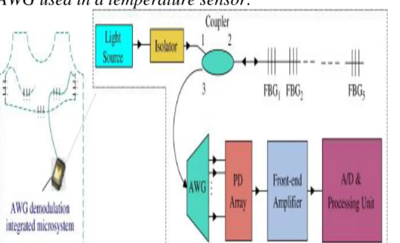
AWG used in a temperature sensor:
Fig 3. Smart clothing containing an AWG and other components used as a device for measuring body temperature. The figure 3 above shows a coat which uses an AWG in a demodulation integrated microsystem to implement temperature sensor. The FBGs are distributed on different locations inside the coat so as to get exposed to the body temperature of the different parts of the body. The light source emits light into a coupler through an isolator that prevents light to be reflected back into the source which might cause instability of the source. The light from the coupler goes to the different FBGs. The
wavelength of the light reflected from the FBGs is dependent on the grating period and refractive index which in turn depend on the temperature over which the FBGs have been exposed. The different wavelengths due to different temperature values are demultiplexed by an AWG then enter an array of photodetectors for conversion to electrical signal. The processing unit is capable of getting the electrical signal from the array of photodetectors and tell what body temperature corresponds to the received electrical signal.
AWG as a wavelength filter:
AWGs can be used as tunable wavelength filters or channel selectors. To be able to do this 2 AWGs are required, 1 to be used as a multiplexer and the other as demultiplexer, they have to be connected back to back and also connected to an array of N amplifiers as shown on the figure below [1] :
Fig 4. The use of AWG as a wavelength filter
The Semiconductor Optical Amplifier (shown on the fig 4 as SOA) can be selectively activated or deactivated depending on which wavelengths we want to filter out and which ones we want to go through. The SOAs which will be activated will have their wavelengths coupled to the multiplexer to the output where as for the ones deactivated will not be coupled to the output and hence considered as filtered.
AWG as a Spectrometer:
Due to its ability to demultiplex incoming light, an AWG can be used as a spectrometer where the incoming light beam can be demultiplexed into its constituent wavelengths. An example is the IOSS device in fig 5 described above [2].
IV. AWG SPECIFICATION PARAMETERS AND DATA ANALYSIS BY USING PYTHON PROGRAMS
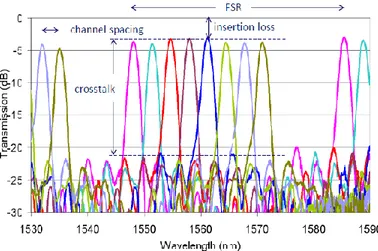
This section gives a detailed description of the parameters which are used to specify an AWG [8]. The aim of this work is to study those parameters/ characteristics for several AWG samples. For each of the below described parameter a python program has been developed in order to compute the parameter. The discussion of each parameter gives an idea of how each of them was implemented by using python programs. To visualize these ideas better I have included a simulation sample spectrum of an AWG in the figure below illustrating some of these parameters.
Fig 5. Spectrum of an AWG showing the different parameters Number of Channels:
This will be equal to the number of receiver waveguides the AWG is designed to work for. It may be 4, 8, 16 …. In the python program it is calculated automatically from the simulation data by counting the number of columns for the output power. Central wavelength:
This is the wavelength that is halfway between the two central channels. It can be calculated as the average of wavelength values corresponding to maximum power of the two central channels.
Channel Spacing:
In AWG spectrum it is the spacing in wavelength between two adjacent channels. It is calculated as the difference between two successive channel’s wavelength values corresponding to the maximum power in each of the channels.
Free Spectral Range:
It is the spacing in wavelength in AWG spectrum between a point in a channel to the same point of the same channel in the next or previous order of an AWG since the spectrum of an AWG is periodic. It can be calculated as the difference in wavelength between the wavelength value corresponding to maximum power of a channel and the wavelength value corresponding to maximum power of the same channel in the next or previous order.
Insertion loss:
This is the loss occurring at the junctions between the free propagation region and the array waveguides due to discontinuity of the free propagation region at the junctions.
It occurs on both the input free propagation region and output free propagation region.
For an AWG since all channels may have different insertion loss so it is important to speak of insertion loss per channel. Insertion loss per channel:
As illustrated by fig 5 above it is a measure of how far the maximum power emitted by a channel is from the reference. It can then be calculated by taking the 0dB minus the maximum power of the channel.
For an AWG it is therefore possible to specify the best insertion loss (the least value) as well as the worst insertion loss (the largest value).
Insertion loss nonuniformity:
In an AWG the channels have different power. The power difference in dB between the maximum power of the channel with highest power and the maximum power of the channel lowest power is the insertion loss nonuniformity. In the AWG simulation data it can be calculated in dB as the difference between the maximum power of the central channel with highest power and the maximum power of the outer most channel with lowest power.
3-dB bandwidth:
It can be defined as the bandwidth of the channel at a point which is 3 dB vertically down from the point of maximum power of a channel. If we draw a horizontal line which is 3 dB vertically down from the point of maximum power it will intersect the curve representing a channel on the AWG spectrum on the right side and on the left side. The difference in wavelength values at the points of intersection of the right and the left will give the 3dB bandwidth.
The 1-dB bandwidth is defined in the same manner with just 3 replaced by 1. Polarization dispersion:
This may be defined as the shift in wavelength of the maximum transmission of an AWG when the polarization of the optical signal through an AWG is changed from TE to TM.
Polarization dependent loss:
It is the difference in output power of the maximum transmission of an AWG channel when the polarization is changed from TE to TM or vice versa.
Cross talk:
There are two types of cross talk in AWGs, general crosstalk and adjacent channel crosstalk.
The general crosstalk can be calculated from figure 3 as the difference between the maximum power of the central channels and the power of the noise or background radiation [9]. It is mainly caused by phase errors due to nonuniformities in layer thickness, waveguide width, and refractive index which cause a noisy “crosstalk floor”
The adjacent channels crosstalk the contribution of the (unwanted) signal at frequency
𝑓
𝑖 to the (detected) channel i. It can be avoided by positioning the receiver waveguides sufficiently far apart. Usually a gap of 1–2 times the waveguide width is sufficient for more than 40 dB adjacent inter-channel crosstalk attenuation. Adjacent channel crosstalk is calculated as the difference between the maximum power of the channel under consideration and the power value of the adjacent channel within the 3dB bandwidth of the channel under consideration.V. MEASUREMENTS IN THE LAB AND ITS DATA ANALYSIS RESULTS
Fig 6. Experimental setup used for doing measurements
Figure
6 shows the experimental setup used in this work. It consists of a tunable laser which produces optical signal that can be tuned over a range of wavelengths (1260nm to 1360nm). The optical signal from the tunable laser enters the polarization controller which is required just to vary the polarization to achieve an optimum reading on the power sensor. The signal then enters the polarization beam splitter which splits the signal into two polarizations, one being TE polarized the other one TM polarized light. The device under test in this case a pigtailed AWG is connected to the beam splitter through its input side (any how would work since the device is reciprocal) and the output side is connected to the power sensor one channel at a time. Before starting any measurement calibration is done by removing the device under test (AWG) and taking the reading on the power meter as well as recording the power emitted by the laser from the laser settings. Then the AWG is then connected to the setup as described above to start the measurements. A Matlab program has been developed to command the laser to start sweeping the wavelengths over the desired range (1260nm to 1360nm) at a certain specified wavelength step (in this case 1nm can give enough resolution) and interval of time(1s). At the same time the detector is commanded by the same program to read the wavelength emitted by the laser at that instant of time. The detector also records and stores the value of the power and its corresponding wavelength on an excel file in a computer connected to both the laser and the detector via GPIB port. When the wavelength sweeping was completed, the data saved in the excel file was accessed through matlab. The data was then prepared in csv formatready for analysis by using python programs.As discussed in the experimental analysis and results subsection below the measurement setup described above which was used to obtain the experimental data used in the analysis leads to some experimental errors. Clearly the above setup needs
improvement to minimize the errors as much as possible. Below are the suggested improvements to be done on the setup to get measured data with much less errors.
i) Getting the proper connector between the pigtailed AWG and the LC fiber end. The connector which is being used now leads to imperfect contact between the fiber surfaces and possibly cause an air gap to exist between the fiber surfaces. The air gap causes losses by reflection and scattering which leads to errors in the measured data.
ii) Polarization converter is needed for switching from TE polarization to TM polarization and vice versa without disconnecting the setup.
iii) After the polarization converter the fiber to be used should be polarization maintaining fiber to avoid any possible changes in polarization which could lead to errors.
iv) A power tap has to be added just at the output of the laser to monitor the laser power and know if there is any laser power fluctuation when measurement is in progress
v) It is necessary to have an array of photodectectors /power sensors whose number will be the same as the number channels of the AWG to avoid disconnecting the AWG every time. The current setup has only one power sensor used for detecting power from all of the four AWG channels, one at a time. In order to be able to detect the power in another channel we need to disconnect the currently measured channel.
Experimental and Analysis Results:
In part one of this project five measurements were taken using the measurement setup described above. Below is a sample spectrum of one of the measurements (Experiment 5):
Fig 7.The spectrum of an AWG for experiment 5 plotted using the measured data(solid lines) and simulation data (dotted lines) Using the calibrated data as input the parameters shown on the table below were computed automatically using a series of python programs.
Table1. The parameters of an AWG for five different measurements performed on the same chip as output by python programs for measured and simulation data
To visualize the difference of the parameters in the above table scatter plots were plotted. Since the parameters are very different in value and too many to be displayed on a single scatter plot they have been put into four groups. Channel spacing, 3 dB bandwidth and 1 dB bandwidth will be in a group known as nm parameters, insertion loss, loss nonuniformity, general crosstalk and adjacent channel crosstalk will be in another group called dB parameters. FSR and central wavelength parameters will be in their separate plots. Below are the scatter plots of those four categories.
Fig 8. Scatter plot to visualize the difference of the parameters channel spacing, 1dB bandwidth and 3dB bandwidth among the five different measurements and simulation
Fig 9. Scatter plot to visualize the difference of the parameters insertion loss, loss nonuniformity,number of channels, general crosstalk and adjacent channel crosstalk among the five different measurements and simulation
Fig10. Scatter plot to visualize the difference of the central wavelength among the five different measurements and simulation
Fig11. Scatter plot to visualize the difference of the central wavelength among the five different measurements and simulation Looking at the above scatter plots we can see that the measured values of the parameters related to insertion loss are somehow different from the simulation ones. This is because in doing these measurements the pigtailed AWG require special connectors which were not available in tha lab, the available connector which was used causes an air gap to exist between the AWG pigtail fiber surface and the other fiber going to the measurement setup. The air gap causes losses by scattering and also by reflection between the two faces of the fibers. This problem can be solved by getting a proper connector as suggested above .
Curve fitting:
A close look of the first passband of the measured spectrum in figure 7 above shows a distorted passband which is very common for most of the experiments. Such distortion which comes as a result of experimental errors and can lead to errors in the values of the calculated parameters due to the algorithms adopted by the python programs.The effect of such distorted passbands can be mittigated by fitting the noisy data using some mathematical function which best describes the passband.Therefore further
improvement in the values of the parameters of insertion loss, loss nonuniformity, channel spacing, 1 dB bandwidth and 3dB bandwidth can be obtained by using curve fitting.
In this case the mathematical model chosen to best describe the passband is a translated parabola with the general equation: 𝑦 = 𝑎(𝑥 − ℎ)2+ 𝑘 (2)
Such a parabola has been translated from the origin to (h,k), where (h,k) are the vertices of the parabola. Since k is the y value of the vertex of the parabola, in a pass band it will correspond to the maximum power of the pass band which is the insertion loss of the channel. The value of ‘a’ tells if the parabola opens upwards (if a>0) or downwards (if a<0). It is known that the pass bands of the measured data open downwards so a<0. The axis of symmetry to the parabola is x=h, in this case the central wavelength of each of the pass bands will be given by its corresponding value of h. Overall central wavelength of the AWG will be the average of the two values of h for the two pass bands in the middle. The 3dB bandwidth can be obtained by substituting for the fitted values of a, h, k obtained from the program and y=k-3 into equation (2) above and solving for x to get two different values of x. The 3dB bandwidth is then obtained as an absolute difference of the two x values obtained.
Below is the table showing the values of a, h and k for each of the four channels before (proposed initial conditions) and after fitting for the data. Channel 1 is in the wavelength range 1260nm to 1295nm, channel 2 is in the wavelength range 1265nm to 1315nm, channel 3 is in the wavelength range 1280nm to 1335nm and channel 4 is in the wavelength range 1300nm to 1355nm.
Table2. Initial condition and optimized parameters of equation (2) for the channels 1, 2, 3 and 4 of an AWG.
Curve fitting is first done to the simulation data by fitting the simulation data to a parabola to be sure that parabola yields a good fit to the simulation pass bands. The results of the fitting to the simulation data are as shown in the passband below , the fitted passband is shown by the black dashed line.
Fig12. Fitted Simulation passbands
From the above passbands it can be seen clearly that the dashed black line (which represents the fitted passband) falls exactly on the dotted lines (which represents the simulation passbands). Therefore the parabola yields a good fit to the simulation data and hence I can proceed fitting the measured data using this mathematical model.
Sample results of the measurement fitted passbands are shown below for experiment 5. Curve fitting is only done on the upper part of the passband in order to mitigate the impact of errors in calculation of the parameters insertion loss, loss non uniformity, channel spacing, 3dB bandwidth and 1 dB bandwidth.
Fig13. Exeperiment 5 fitted passbands shown by black dashed lines
After fitting the measured data using the described mathematical model with the parameters described above the results shown on the table below were obtained.
Table3. The differences in the obtained parameters in the above table can be visualized using below scatter plots
Fig14. nm parameters scatter plot visualizing the difference in the parameters obtained after curve fitting.
Fig15. dB parameters scatter plot visualizing the difference in the parameters obtained after curve fitting.
Comparison of fitted versus non fitted parameters shows that the spreading of the measured parameters on the scatter plots of the fitted parameters is reduced. This is a desirable feature because it shows stability of the corresponding AWG parameter among the different AWGs.
Further the difference between the simulated and measured values for the fitted parameters is reduced.
For 3 dB bandwidth the simulation value of the first channel was way lower than measured values which was wrong and did not make sense with the unfitted data, the problem has been corrected in the fitting.
Before fitting some of the measured values for 1 dB bandwidth were higher than the simulation values which doesn’t make sense, fitting has cleared the problem.
VI. ANALYSIS OF DATA OBTAINED FROM STOCK
This part works on the analysis of data of 6 different types of AWGs with 28 AWGs from each type. 28 different measurements were performed, in each measurement the six types of AWGs were compared and in each type of AWG only one channel of the AWG was measured in a measurement. The types were named as AA, AB, AC, BA, BB and BC expected to be in decreasing order of quality due to the way they were designed. The AA, AB and AC were designed in such a way that the AWGs were separated from each other in position and hence better etching was possible during fabrication. For the AWGs types BA, BB and BC the AWGs were tightly positioned next to each other such that the etching efficiency was not so good and hence relatively poorer performance of the AWGs was expected. The different AWG types appeared to have either a spectrum that is split (true for AB, BA, BB and BC) or a non split spectrum (true for AA and AC) as shown in the figures below.
Fig16. Non split spectrum
Fig17. Split spectrum
To evaluate the performance of the different AWG types the following parameters were computed and used for performance comparisons of the AWG types:
i. The wavelength of the channel that has peak power ii. The distance between the main peak and side peak
iii. The power difference between the main peak and side peak
iv. The difference of the main peak of each AWG type from the maximum of the main peaks of all the AWG types in an experiment.
The first three can easily be visualized from the split spectrum as follows i) The wavelength of the channel that has peak power:
All the power values of a channel were stored in a numpy array and the maximum value in the array was found. The value of wavelength corresponding to this maximum was calculated using argmax function in python. For good performance of an AWG it is desirable that the wavelength at which the peak power happens doesn’t vary much when different AWGs of the same type are measured so that the central wavelength remains to be nearly the same for all AWGs.
To visualize the difference of this parameter among the 6 different AWG types for the 28 measurements we can use the scatter plots and box plots below.
Fig18. Scatter plot of peak power wavelength against the AWG type for the 28 different measurements. Below is the box plot of the above scatter plot:
Fig19. Box plot of peak power wavelength against the AWG type for the 28 different measurements
As stated above for this parameter it is desirable that the points of the scatter plot don’t spread much thus looking at the above box plot AA has the least spread since it has the smalllest box followed by AC the rest of the boxes are large in the order BA, BB, AB and BC.
ii) The distance between the main peak and side peak:
From the values of power stored in a numpy array explained in the first parameter above the function argrelextrema is used to get the indices of all local peak powers in the numpy array. The local peak power values are then stored in a list arr. The list is sorted in an increasing order, such that the overall maximum peak power (main peak) is the last element of arr i.earr[-1] and the next high peak power (the side peak) is in the last but one element i.e arr[-2] .Searching through the numpy array storing power
values will help to know the index of the numpy array having the value of arr[-2], then using this index the corresponding wavelength can be obtained by putting that same index in the array storing the wavelength values. The difference between this value of wavelength and the wavelength corresponding to maximum power gives the value of the distance between the main and side peaks. For good performance of an AWG it is desirable that the distance between the main peak and side peak is as high as possible so that the side peak can have much less impact on the main peak.
To visualize the difference of this parameter among the 6 different AWG types for the 28 measurements the scatter plots and box plots below can be used.
Fig20. Scatter plot of the distance between main peak and side peak against the AWG type for the 28 different measurements. Below is the box plot of the above scatter plot:
Fig21. Box plot of the distance between main peak and side peak against the AWG type for the 28 different measurements. As stated above for an AWG to perform well it is desirable that the distance between the main and side peak is as large as possble. Looking at the above box plot, the mean value shown by the green can be used to tell the value of this parameter, looking at the box plot AA has the highest value of this parameter followed by AC then BB and then BC, BA and AB.
iii) The power difference between the main peak and side peak:
From the above explanation the power difference between the main peak and side peak is obtained as the difference between the values arr[-1] (power of the main peak) and arr[-2] (power of the side peak) . For good performance of an AWG it is desirable that this power difference is as high as possible since the side peak is undesirable due to the crosstalk it causes to the main peak.
To visualize the difference of this parameter among the 6 different AWG types for the 28 measurements the scatter plots and box plots below can be used.
Fig22. Scatter plot of power difference between the main peak and side peak against AWG type for the 28 diffetent measurements.
Below is the box plot of the above scatter plot:
Fig23. Box plot of the difference between the main peak and side peak against AWG type for the 28 diffetent measurements As stated above for an AWG to be considered as a good one it should have a high value of this parameter, looking at the mean shown by green line in the above box plot, AA has the highest followed by AC and then BB and lastly BC, BA, AB in that order.
iv) The difference of the main peak of each AWG type from the maximum of the main peak of all the AWG types in an experiment:
To better describe this parameter I will consider the spectrum of one of the measurements which consists of the spectrum of all the six AWG types plotted together as shown below:
Fig24. Spectrum of the six AWG types compared in one of the 28 measurements
From the above spectrum it can be seen that the AWG type AC (red color) has the maximum power of all the other types. This metric is meant to calculate how much below this maximum each of the maximum power of the other AWG types is. So this parameter is calculated by taking the maximum of peak power of all the AWG types (in this case is the peak power of the AC type) minus the peak power of each AWG type. As seen from the spectrum the next one is AA. In fact AA and AC have good performance because the value of this parameter is small. Thus the smaller the value of this parameter the better the performance of the AWG. The rest of the types like AB, BA, BB and BC have relatively high value of this parameter and hence have
relatively poorer performance.
To visualize the difference of this parameter among the 6 different AWG types for the 28 measurements the scatter plots and box plots below can be used.
Fig25. Scatter plot of difference of channel peak power frommaximum peak power against AWG type for the 28 diffetent measurements.
Fig26. Box plot of difference of channel peak power from maximum peak power against AWG type for the 28 diffetent measurements.
For a good AWG the value of this parameter has to be low. Looking at the mean shown by the green line in the above box plot AC has the lowest value, followed by AA then BC, BB, BA and AB in that order.
A general conclusion which can be reached is that the AWGs AA and AC are good and hence will have good performance where as the AWGs AB, BA, BB and BC are bad and will have poor performance.
VII. AUTOMATINGTASKS AND ANALYSIS STEPS
One of the main goals of this project is to automate tasks. This is because in most cases companies manufacturing AWGs usually manufacture many AWGs and hence the number of AWG chips to be characterized is normally large. It would be difficult, boring, time consuming and errors prone if some of the tasks were done manually. In automating tasks with the measurement setup described above there was a big challenge of synchronization which was faced at the beginning when the laser was commanded from its buttons to sweep the wavelengths and separately at the same time the detector was commanded to record the readings. This synchronization problem was solved by commanding the laser and the detector simultaneously by using a single matlab program.
In performing measurements, one of the tasks where automation is done is in sweeping the wavelength from 1260nm to 1360nm at an interval of 1nm with a delay of 1 second. The second task automated is on the power sensor to read and display the power and the wavelength when the wavelength sweep is in progress. Data saving on an excel file is also automated where the values of power and their corresponding wavelengths received by a power sensor are recorded and saved. All the automation tasks
mentioned so far are done by a single matlab program which was developed as a part of this work.
The task of automatically determining all parameters of an AWG is done by using python programs. Python programs have been developed to compute automatically all the parameters discussed in section IV above. The input to these programs is the name of the csv file containing the calibrated measurement data which include the output power of each channel and their corresponding wavelength values. The output will be automatically exported to an excel file (all the 12 parameters discussed in part IV above) for each AWG. The number of excel files which are as many as the number of characterized AWGs are produced automatically by a single python program. The data exported to excel is in the form of a list and so no operation can be performed on them when having that form. So a python program to automatically split the list into its constituent elements for all the excel files produced by the previous step was developed. The next program took all the split parameters excel files discussed above and merged all the parameters into a single excel file in a tabular form giving table1 in section V. Using this excel file with data in table 1 as input a python program to automatically display the scatter plots discussed on section V above was developed. Below block diagram summarizes the analysis steps described above.
Fig27. Block diagram to summarize the data analysis steps by pthon programs CONCLUSION
The analysis procedures have to a large extent proven to be effective and automatic in determining the required parameters of an AWG. In the first part only five experiments and simulation data were analyzed but the analysis can easily be made scalable to any large number AWGs to be characterized by changing only few parts in the python programs. Testing the scaling up of the AWGs to be characterized, the second part of the work did a successful analysis on a total of 168 AWGs using similar python programs to those used in part one with just little modification on few areas of the programs. From the measurement setup point of view, despite having all the automation described in section VII, it still needs more improvement to become more automatic with minimized measurement errors as suggested in section V of this paper. After the suggestions on improving the measurement setup given in section V are implemented, it is my strong belief that through this work we will have achieved a measurement setup and analysis procedures which are effective and automatic enough to do characterization and analysis of any large number of AWGs with less hassle.
ACKNOWLEDGMENT
I would like to express my sincere thanks to my supervisor Dr. Nicola Calabretta and my co supervisor Dr. Ronald Brooke for their continuous support which they gave me in accomplishing this work.
REFERENCES
[1] Leiijtens X.J.M,Kuhlow.B & Smit,M.K “Arrayed Waveguide Gratings. Wavelength filers in fiber optics pp. 125–187” 01 January 2006. [2] Gloria Micó, “Integrated Optic Sensing Spectrometer:Concept and Design” . 27 February 2019
[3] P.Cheben “A high-resolution silicon-on-insulator arrayed waveguide grating microspectrometer with sub-micrometer aperture waveguides”. 22 February 2007
[4] Meint K. Smit, “PHASAR-Based WDM-Devices: Principles, Design and Applications” JUNE 1996.
[5] Daoxin Dai “Low-loss silicon nitride arrayed-waveguide grating (de)multiplexer using nano-core optical waveguides” 08 July 2011 [6] Jia Jiang “Arrayed Waveguide Gratings Based on Perfluorocyclobutane Polymers for CWDM Applications”. 28 October 2005
[7] Jingyao Li, Rui Yin, Wei Ji, “AWG optical filter with tunable central wavelength and bandwidth based on LNOI and electro-optic effect” 26 August 2019 [8] D. Seyringer and M. Bielik, “AWG-Parameters: new software tool to design arrayed waveguide gratings” 2013
[9] Daan Martens , “Compact Silicon Nitride Arrayed Waveguide Gratings for Very Near-Infrared Wavelengths” 17 October 2014 .
[10] S. T. S. Cheung1, B. Guan1, S. S. Djordjevic1, K. Okamoto2 “Low-loss and High Contrast Silicon-on-Insulator (SOI) Arrayed Waveguide Grating” May 2012
[11] Pradip gatkine,Sylvain Veilleuxa, “Arrayed waveguide grating spectrometers for astronomical applications: first results” 2006.
[12] Pradip gatkine, “Arrayed waveguide grating spectrometers for
astronomical applications: new results” 18 Jul 2017
[13] Zhao Lei, “16 channel 200 GHz arrayed waveguide grating based on Si nanowire waveguides,” February 2011 [14] Daoxin Dai, “Mode conversion / coupling in submicron silicon-on-insulator optical waveguides and the applications,”