1
A spatial econometric analysis of land use efficiency in large and small
municipalities
Abstract
We estimate the relationship between urban spatial expansion and its socio-economic determinants in Lombardy, the most urbanised region of Italy (and one of the most of the European Union), at the municipality level. Test results suggest that this relationship varies significantly among municipalities of different size and findings support the hypothesis that larger ones are more efficient in managing land take. In particular, we find that the marginal land consumption per new household is inversely related to the size of the municipality and we link this evidence to the fact that, since more space is often available, small municipalities pay less institutional attention to the issue of land take and consequently internalise less the environmental externalities. This evidence calls for a reflection on the role of planning policies and the effectiveness of undifferentiated measures to contain land take, especially in the case of Italy, where the municipalities, more than 99% of which have less than 50,000 inhabitants, decide on land use transformations.
Keywords: Land take; city size, threshold regression; spatial econometrics JEL: O18;Q15; R14
1.INTRODUCTION
Is the inefficient land use related to city size? With about 7.6% of land classified as artificial, against the European Union (EU) average of 4.6%, Italy is among the countries in Europe where the problem of land take is most severe. Like in many other countries, urbanisation – meaning industrial, commercial, and residential land use and transport infrastructures – is the main responsible of this land take, which primarily realises at the expenses of agricultural land. According to the last report of soil consumption in Italy (ISPRA, 2015), infrastructures and urban fabric account in fact for 41% and 30% of total land consumption respectively, hence the conversion of land from mainly agricultural (60%) and natural (20%) uses to urbanised area. Italy is a highly fragmented country from the administrative standpoint: large municipalities, with more than 50,000 inhabitants, represent less than 2% of the total (about 8,000) municipalities. With more than 30% of the Italian population, large municipalities concentrate less than 20% of the total artificial area: this means that medium-size and small municipalities, where the average population density is lower, are also mainly responsible for land take. For instance, more than 30% of the artificial area concentrates in municipalities with less than 5,000 inhabitants. The urbanization-driven land use change often impacts the environment and the ecosystems significantly. Hence, it is regarded as socially undesirable, especially by civic and political groups wishing to preserve the territory from soil sealing, as well as from noise and pollution generated by the transport system. Larger cities imply longer average commutes, more substantial air pollution and road congestion and, in turn, the deterioration of the environmental quality and the quality of life of individuals and communities. Studies documented also the effects on the ecological equilibrium (Alberti, 2005) and the potential for rural development, primarily through the direct effects on farmland loss and indirect effects on farmland prices (Delbecq et al., 2014; Guiling et al., 2009; Karlsson and Nilsson, 2014; Livanis et al., 2006).
2
Urban economists traditionally mitigated this strong negative sentiment against urban expansion upholding a rational justification for it, connected to the increased demand for housing generated by higher income, growing population, and the decline in transport cost (Brueckner, 2000). Grounding on the Mills-Muth theory of monocentric urban development (Mills, 1972; Muth, 1969), the economists' view advocates the predominant role of market forces in determining the optimal allocation of land across alternative uses, which benefits the households to the largest extent. Building on the comparative static analysis elaborated by Wheaton (1974), Brueckner and Fansler (1983) propose a regression approach to testing if some exogenous variables influencing the demand and supply of housing can explain the spatial size of cities. Their results provide support and justification for the economists' view, implicitly rejecting the hypothesis of sprawl, intended as a consumption of land not explained by a utility-based economic rationale. McGrath (2005), Paulsen (2012), Spivey (2008), and Wassmer (2006) extend this stream of empirical research on different samples of US cities. US-based evidence suggests that the variables of the Mills-Muth model, namely population, income, transport costs and agricultural rents, explain about 80% of the spatial variation in the urban city size (Paulsen, 2012). Results are similar in some European countries (Hortas-Rico, 2014; Oueslati et al., 2015; Pirotte and Madre, 2011) and in developing countries such as China (Deng et al., 2008; Song et al., 2014) and India (Brueckner and Sridhar, 2012).
Despite the robust empirical evidence endorsing the role of markets, the optimal land allocation is still influenced by externalities that may prevent the correct functioning of market mechanisms, impacting both the average and the marginal land consumption as well as the geographical distribution of urbanisation. For instance, landscape is a public good and its value is not considered an economic loss in the conversion of agricultural (or natural) land for real estate purposes. Congestion likewise causes negative externalities that the commuters are not asked to pay for in the cost of their trip. In theory, the cost of externalities could be internalised, as suggested by Brueckner (2000), but in fact, the use of a system of fiscal incentives as a remedy to market failures can be very difficult to implement and to manage in the case of land use (Knaap et al., 2007). As a partial result of market inefficiency, urban spatial expansion occurred even in circumstances of declining population and number of households (Haase et al., 2013). Often, in the past, local municipalities planned urban spatial expansion through greenfield building in response to a growing population. Less often, and more recently, some attention converged to the practices of residential densification (brownfield building), the process of urban restructuring functional to accommodate the increase in the demand for houses within the existing urban space (Broitman and Koomen, 2015). Densification is associated to a regain in residential attractiveness and occurred primarily in few inner-cities (Haase et al., 2010). Hence the cities become larger and their density lower, especially in the peripheries, for reasons that are weakly related to the socio-demographic trends. In contrast, evidence indicates that people value the high fragmentation of residential land use (Kuethe, 2012), which increases the demand for houses in the peripheries. Consequently, the controversial dispute about the call for urban planning practices is still unresolved, opposing those who believe that densities at the urban fringe are remarkably low to the detriment of agricultural and natural land and that the urban
3
densification should be encouraged, and the expansion discouraged, to those who consider that the restrictions about land-use will only narrow people's utility by limiting housing supply.
The divergences in the definitions of sprawl and the methods to assess the relevance for urban expansion of market-related factors contribute to fuelling this controversy. On the one hand, in defining sprawl, many (usually land-take opponents) refer to the mere increase in urbanised area (Patacchini et al., 2009), which is seen as a bad result independently from the extent to which is effectively driven by a growing demand for housing. Others refer more specifically to the fragmentation of the built-up area (Oueslati et al., 2015). In contrast, economists define sprawl as a land take that is excessive with respect to the optimal amount of urbanised area, and specifically to housing demand (Brueckner, 2000). In line with this approach, the OECD suggests measuring sprawl as the growth in built-up area adjusted for the growth of population (OECD, 2013). Furthermore, the economists' view recognise the peculiar character of urban sprawl, outlined primarily by declines in housing unit density and by increases in marginal land consumption per new household (Paulsen, 2014). On the other hand, regarding methodology, the Brueckner and Fansler (1983) approach only shows that urban size is related to market variables but does not reveal to what extent this relationship leads to consumption of land that could be defined excessive. To evaluate this point, consider the case of population, which probably has the largest impact on housing demand. Some cities respond to population growth encouraging densification and planning only small, and very dense, expansions; some other cities promote low-density building beyond the urban fringe. In both cases, the increase in urbanised area can be linked to population growth, but only in the second case the expansion takes the characters of sprawl, hence declining density and increasing marginal land consumption.
In this work we argue that the Brueckner and Fansler (1983) approach provided so far clear indications in favour of the economic rationale behind urban spatial growth, and implicitly against the hypothesis of excessive land take, since focused on large cities and metropolitan areas, while excluding the low-density peripheries (see Paulsen (2014)), and neglecting medium and small cities. In particular, we suggest that the price of land in large cities better internalises the negative externalities implicit in the process of land use change. Oppositely, unnecessary land take and sprawl phenomena likely appear in small cities, where the availability and the low price of land often lower the institutional attention on its efficient allocation and on the necessity to balance the negative environmental externalities. For instance, the countryside, which supplies open spaces and rural and natural amenities, is readily available in cities of limited size, and the urban landscape is hence less valuable. Moreover, the increase in commuting is not perceived as a problem, since urban traffic is still at levels which do not cause excessive congestion and air pollution. More available space and less institutional attention lower the competition for land use with two most important implications. First, an increase in income makes people more willing to leave their apartments in the city centre to buy larger houses in the periphery, determining an increase in urbanised area which is not motivated by the demographic dynamics. Second, relatively lower land prices translate into more substantial profits for the building sector,
4
stimulating the speculative behaviours of agents that also leverage on the lower fiscal capacity of the municipalities and on their need to use land conversion charges to finance their budgets.
We assess the structural differences in the behaviours of large and small municipalities using the case study of Lombardy region, the most urbanised region in Italy (and one of the most urbanised in the European Union). We build the analysis at the municipality level, because each municipality – regardless of the size – can decide (substantially) by itself on land transformations affecting its territory, and show that large municipalities are relatively more efficient in managing land use compared to medium-size and small ones. This evidence of relative inefficiency provides little support for an economic rationale behind the urban spatial expansion. On the contrary, the findings in this paper call for a deeper understanding of the territorial determinants of urban expansion, especially in those areas traditionally marginalised by the sprawl debate, to provide more effective policy instruments.
In the next section, we discuss the features of the Italian administrative structure, justifying the attention to the municipality level. Next, we illustrate the empirical model (section three), describe the data used (section four) and the empirical results (section five) and discuss the implications of these results in the conclusion (section six).
2.SPATIAL PATTERNS OF LAND USE IN ITALY
Italy is a country characterised by a high administrative fragmentation, with 20 (NUTS12) Regions, 110
(NUTS3) Provinces and 8,000 (LAU1) municipalities. The State and the Regions define the main regulatory frame for the planning policies, which are in fact differentiated by Region. The current legislation, however, puts the municipalities at the centre of the decision-making process concerning planning policies. In particular, the city council allows land use transformations through a land plan, establishing which zones are eligible for urbanisation; which type of transformation (residential, industrial, commercial) can take place; and the volumetric limits allowed. It follows that the national representation of the urbanisation processes is the result of the planning choices made by 8,000 decision-making centres that have the same power independently of their size, in terms either of surface or number of inhabitants.
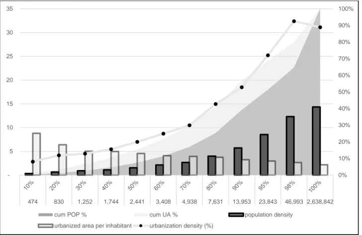
The vast majority of municipalities in Italy are small, with less than 5,000 inhabitants, and this clearly impacts urbanisation. Figure 1 illustrates the relationship between population and urbanisation for the different size percentiles: the horizontal axis indicates the percentile of population distribution and the associated absolute values. We compare the cumulative distributions of population and urban area (values in the right scale) and note that the cumulated urbanised area is always larger than the cumulated population in the graph but, in particular, the difference between the two areas widens in municipalities between 3,500 and 47,000 inhabitants. Not surprisingly we find that the group of municipalities with less than 3,500 inhabitants, which represents 60% of the total but only 11.5% of the total population, accounts for about 22% of the urbanized area, and the
5
group of municipalities with between 3,500 and 47,00 inhabitants, which represents 38% of the total and 53% of the population, accounts for 55% of the urbanized area.
Figure 1 about here
According to ISPRA (2015), in the last 60 years, urbanisation in Italy lost the connection with demographic changes, as soil consumption per new household more than doubled at the national level, increasing from 167 to 345 square meters per inhabitant. Such an increase is, at least in part, related to the spatial structure of municipalities, being the population density substantially lower in small municipalities compared to large ones. The possibility of low-density urbanisation also determined different urban morphologies, since a higher degree of urban fragmentation is found in small municipalities (ISPRA, 2015). From the figure emerges a positive relationship between urbanisation density (urbanized on total area) and population density (population over total area). However, with increasing urban size, the urbanised area grows proportionally less than population and, in fact, we note in the figure that the quantity of urbanised area per inhabitant in inversely related to the size of the municipality.
Hence, in Italy, as in many other countries, a substantial part of urbanisation geographically concentrates in few large municipalities. Still, the majority of urbanisation involves the medium-size and small municipalities and especially the very small ones where the share of urbanised area in unreasonably high and where the link with demography appears very weak.
3.METHODOLOGY
The empirical approach of economists to model the size of cities in relation to market forces derives from the tradition of Central Business District (CBD) models developed by Mills (1972) and Muth (1969). In this model, consumers maximise the utility associated with housing preferences and the consumption of goods subject to a budget constraint. The income earned as compensation for labour is spent for the ordinary good, the housing good and, also, the house-to-work commuting. Since the unitary cost of commuting is fixed, the total commuting cost for the household depends uniquely on the distance of the house from work. Furthermore, the price of the housing good lowers at larger distances from the CBD, where all the jobs concentrate. Based on these simple assumptions, the individuals make their optimal choice trading off between the quantity of housing (how large the house should be) and the cost of commuting (how far to live from the centre). In equilibrium, all the individuals have the same level of utility: people living far from the centre incur higher transportation costs, which the lower price of houses and the possibility to live in larger houses compensate. The size of the city is the optimal one and in the urban fringe the marginal return from real estate equals the marginal return from the agricultural activity. Wheaton (1974) summarises the main outcome of the model through the following set of comparative statics:
(1) 0; 0; 0; 0
u u u u
6
It is postulated that the equilibrium size of a city
u
positively depends on the total population
p
and the average income
i
, and negatively on the average value of agricultural land
r
in the urban fringe and the cost of transportation
t
. The economic insights behind the comparative statics are intuitive. An increase in the urban population shifts up the demand for housing and the house prices, forcing some people to move to the urban fringe to pay relatively less. As the willingness to pay for a house at the urban fringe increases, the marginal return from building exceeds that from agricultural activities, resulting in an urban expansion. An increase in income also shifts the demand for housing and causes urban expansion since with more income available households will demand larger houses. An increase in the price of agricultural land makes the city more compact because the higher housing price at the urban fringe lowers the households' gain in utility from moving far from the centre. An increase in the cost of transportation generates the double effect of discouraging commuting and of shifting down the demand for housing through a decrease in the disposable income for the housing good. With less income to spend on housing and lower willingness to commute, more people will leave close to the city centre.Brueckner and Fansler (1983) convey these insights into a simple model to be estimated econometrically for a cross-section of cities to measure how much of the variation in urbanised area could be explained by the market mechanisms described by the CBD model:
(2) u
0
1p
2i
3t
4r e .The model represents the starting point for the analysis of urban sprawl:
u
is the vector of the spatial extents of urbanized areas, measured in square kilometers or hectares;p
,i
,t
, and r are the vectors of independent variables, respectively total population of the city, average household income, a proxy for transportation costs and a proxy for agricultural land values. Holding the standard hypothesis of the linear model on the zero-mean and constant variance i.i.d. error terme
, the
parameters can be estimated via OLS. In particular, the hypothesis of uncorrelated residuals is expected to hold when comparing cities spread across a vast territory because the behaviour of a city is not suspected to influence that of the other cities, except for some impact of national and regional effects for which the regression should control for.The hypothesis of uncorrelated residuals is likely to be violated by the presence of territorial spillovers, when the cross-section sample includes contiguous areas, resulting in biased estimates of the model parameters. This is, specifically, the case of this paper because the theoretical Mills-Muth model is tailored on the conceptualisation of the city as a large urban agglomeration that includes the main municipality and also the geographically and functionally related ones and the actual empirical model is estimated using municipality data instead. Hence, we can expect a certain degree of interconnection between municipalities, especially in the nearby of urban agglomerations, as predicted by the Mills-Muth model. For instance, the commuting workers of the model face a trade-off between the house price and the commuting cost but, in picking the best location to live in, they generally look outside the border of the workplace municipality, because houses are
7
cheaper and maybe cross-municipality commuting is also less expensive, in terms of both time and cost, than commuting from the edge to the centre of the municipality. Additional justifications for the presence of spatial spillovers recall the structure of house prices and their transmission that, independently of the theoretical model predictions, overlap the administrative borders of neighbouring areas. The approach in this paper considers the geographical nature of these relationships but we cannot exclude that more complex dynamics related to functional linkages and hierarchical dependence may be more relevant2.
Spatial econometric models (Anselin, 1988a) are set up accounting explicitly for spatial spillovers in econometric modelling using a spatial contiguity matrix
W
, whose elements express the geographical contiguity relationships between the units in rows and columns. The spatial matrix is usually row-standardized in a way that, when it pre-multiplies a variable, it returns the average value of the variable in the neighbours. LettingX
[ , , , ]
p i t r
be the matrix of the model covariates and
T
1,
2,
3,
4
the vector of related coefficients, the model in equation (2) can be rewritten in compact form as u
0X
e. Common specifications of spatial econometric models are generalised restrictions of the Manski (1993) model:(3)
0
u Wu X WX ε ε Wε e .Spatial effect may enter endogenously through the spatial autoregressive term
Wu
to reflect the impact of urbanization in neighbours, exogenously to reflect the consequence for each unit of the change in exogenous variables
WX
, or may affect the unexplained part of the model through a spatial autocorrelation structure
Wε
due to unobserved environmental effects common to neighbouring units (Elhorst, 2010).As suggested by Manski (1993) and confirmed by Elhorst (2010), the spatial model in equation (3) cannot be estimated unless one out of the three spatial parameters
, ,
is set to zero. Otherwise, the parameters are not identified. LeSage and Pace (2009) suggest that, in general, excluding the spatial autocorrelation term is the best strategy because it preserves the estimates from the omitted variable bias problem. However, spatial heterogeneity turns out to be a crucial aspect of city size models. In particular, the predictions of the monocentric models describe an equilibrium condition which also reflects additional sources of spatial heterogeneity over which households have specific preferences (Irwin, 2010 p77). Such preferences are related, for instance, to the presence of local public goods such as open spaces (Turner, 2005; Wu and Plantinga, 2003), environmental amenities (Tajibaeva et al., 2008; Wu, 2006), or a combination of both (Kovacs and Larson, 2007), and agricultural amenities (Coisnon et al., 2014), and are likely clustered in space. Since we do not observe such features in our data, we are confident that unobserved spatial heterogeneity is2 While functional/hierarchical connectivity structures can probably best account for non-spatial configurations of the
system of relationships and a comparison of the results using differently constructed matrices can provide interesting insights, we leave the issue for future research because it is not strictly related to the objective of this research, which is the difference in land use efficiency in small and large cities.
8
an important issue in the econometric estimation and should be considered appropriately. In support of this, we conduct robust LM tests (Anselin, 1988a) on the linear model, and the results provide relatively stronger evidence for the spatial autocorrelation structure
0
compared to the spatial autoregressive structure
0
. In the spatial econometric literature, the model we estimate is labelled as Spatial Durbin Error Model3: (4)
u X WX Z ε ε Wε e .In addition to the standard market-related variables suggested by the theoretical and empirical literature, some additional control variables
Z
are included. The choice to exclude the spatial autocorrelation term and to include the spatial lag of the explanatory variables brings computational advantages in the estimation of the spillover effects
u
/
Wx
and the variance-covariance matrix (LeSage and Pace, 2009 p41), in particular when the coefficients may present structural instability as we suspect for this case.Structural instability of the coefficients and more specifically heterogeneity in some slope parameters is a very important issue in econometric models, and it is also highly relevant in the context of city size models because the market forces determining the equilibrium city size may operate differently in large and small cities. Structural instability is conventionally approached defining regimes or groups or sub-samples of observations characterised by a specific feature, and estimating multiple sets of group-specific slopes. Ex-ante sample splitting requires some knowledge about the nature of splitting, which may ground on theoretical arguments, as in the case of models explicitly allowing for multiple equilibria, or on the empirical observation of non-linearities in the effect of the covariates. This knowledge is further conveyed into a set of dummy variables to be used for sample splitting, modelling group-wise heterogeneity in slope parameters.
When the nature of splitting concerns a continuous variable, a convenient approach to identify the regimes is the threshold regression procedure suggested by Hansen (1996, 2000) for linear models. The method works as follows. Having defined a threshold variable, the population
( )
p
in our case, them
unique values of the variable are selected and, for each value, a dummy variable dm
pi p*m
is generated equal to one if the population of the city
p
i is larger than that critical value
p* . The following model:
3 Actually a pure Spatial Durbin Error Model would include also the spatial lags of the control variables. We restrict the
application of spatial lags only to the variables suggested by the CBD theory and employed in the previous empirical literature.
9 (5) 0 1 0 1 m m
u X WX Z ε ε Wε e d dis then estimated via standard Maximum Likelihood procedures
m
times and the concentrated sum of squares
*m m
S p are stored in an
m
-dimensional vector. The estimator of the threshold p1 is the value of p*m that minimises Sm
p*m .Having defined the thresholdp1, the model in the equation (5) is estimated with dm d1
pi p1
. Hansen (1996) argues that the procedure to test the null hypothesis of structural stability
1
1 0
when the threshold value is not known apriori cannot be a simple Wald test because the threshold parameter is not identified under the null hypothesis; thus, he suggests alternative Likelihood Ratio based tests for linear models. The test for structural instability in spatial models conducted here is the Likelihood Ratio based spatial version of the Chow test (Anselin, 1988, 1990) that compares the full model (with the threshold) with the restricted one (without the threshold).After a rejection of the hypothesis of structural stability, the search continues for the second threshold. Using the
m
1
values of the threshold variable, a new dummy variable is generated dm
pi pm*
, taking positive values if the population is above the threshold. This new dummy is used in the model:(6) 0 1 1 2 0 1 1 2 m m
u X WX Z ε ε Wε e d d d dand the estimator of the second threshold, p2, is the value of
p
that minimises Sm
pm* | p1
.After finding the value of the second threshold, the model in equation (6) is estimated substituting
2 2
m i
d d p p , and the spatial Chow test is conducted comparing the unrestricted model (with two thresholds) with the restricted model (with one threshold). The search then continues for additional thresholds and stops whenever the spatial Chow test rejects the hypothesis of further structural instability.
4.DATA
We conduct our empirical analysis on the municipalities of the Lombardy region in Italy. Lombardy hosts the second largest Italian city, Milan, and this favoured the rapid economic growth of the last decades. Such growth
10
was accompanied by relevant infrastructural investments and today the territories of the region, about 24,000 km2, are connected by a network made of more than 600 km of motorways and more than 11,000 km of other roads4.
Growth and infrastructural development determined substantial consequences regarding the spatial expansion of urbanisation. To date, 14.5% of the total regional territory is urbanised land, almost twice the national average. The figure was estimated at 12.6% in 1999, meaning that approximately 45,000 ha of land has been urbanised in less than 15 years. 90,000 square meters, almost nine football fields, of agricultural and natural land are being lost every day to leave space for commercial and residential areas5. In the meanwhile, the
population increased, but less than proportionally, and the average density in 2012 was 180 inhabitants per ha. Such a trend is clearly unsustainable in the long run, especially considering that urbanisation and land use change are concentrated in tiny portions of the territory, among which, of course, the Milan area.
There are 1,543 municipalities in the dataset, which are very heterogeneous regarding population. For instance, Milan is the largest municipality, with more than 1,250,000 inhabitants, followed by Brescia (191,465) Monza (119,890) and Bergamo (115,499). Only 14 municipalities have more than 50,000 inhabitants and more than 50% of the municipalities in the sample have less than 3,000 inhabitants, largely below the sample average. Table 1 summarises the whole distribution through the values of the deciles. Overall, the distribution of the population, which is the threshold variable in this model, is notably concentrated in the left tail, with a very long and thin right tail.
Table 1 about here
Table 2 describes the variables employed in the model and presents also the sample mean and the standard deviation. The dependent variable
( )
u
is the urban municipality size and is measured as the sum of the residential, commercial and industrial area. Among the explanatory variables, those predicted by the theoretical model and widely employed in the literature are the total population living in the municipality( )
p
and the average income earned by households in the municipality( )
i
6. Although predicted by the theoretical model,agricultural land values
r
and transport costs
t
are less frequently employed in the empirical estimation because there are no sufficiently valid proxies. Here we measure transportation costs as the inverse of the number of cars per inhabitants and agricultural land values as farmland values. Relatively to transportation costs, we follow Glaeser and Kahn (2004) who suggest that cars reduce transportation costs and that, in fact, the increased speed of urbanisation is, at least in part, the consequence of the easier and cheaper commuting4 Source: elaborations made by the Italian Government - MIT (Ministry of Infrastructures and Transport), ANAS
(Motorways Management Society) and ISTAT (National Institute of Statistics). Data available at http://www.asr-lombardia.it/ASR/regioni-italiane/trasporti/reti-infrastrutturali-e-impianti/tavole/1679/2012/.
5 More details at http://lombardia.legambiente.it/temi/territorio/consumo-di-suolo.
6 More recent evidence suggested that urban growth has differentiated effects on spatial expansion depending on
individual sectors and growth mechanisms (Burnett, 2012) and, accordingly, median income may be a poor proxy of the economic development of a city. Nonetheless, in absence of more detailed information on the economic structure of cities, we follow the empirical literature that uses median income.
11
introduced with the diffusion of cars7. Concerning agricultural land values, the national institute of agricultural
economics releases statistics on farmland values at the provincial level8 and by type of crop. The farmland
value at the municipality level corresponds to the weighted average of the prices of land for different crops, using the municipality level area shares as weights; this guarantees sufficient variation in the value of this variable, especially among municipalities in the same province9. To control for additional variation in urban
size not explained by the covariates, we include some control variables expected to capture the incidence of physical infrastructures and the presence of construction sites.
Table 2 about here
5.RESULTS
Table 3 summarises the estimation results for the city size model in the absence of threshold effects using four different models. From left to right we present the linear model, which does not consider the spatial effects; the Spatial Durbin Error Model (SDEM), which includes all the spatial lags of covariates but the controls and, in addition, assumes spatial autocorrelation of the disturbances; the Spatial Error Model (SEM) which assumes a spatial autocorrelation of the disturbances only and, finally, the Spatial Lag Model (SLM), which assumes a spatial autoregressive dependent variable. For the estimation of all the models, the same contiguity matrix
W
is used. This is constructed assuming that all the municipalities within a given distance band from the origin municipalities are considered neighbouring, and the distance band is selected in a way that each municipality has at least an adjacent one. The inverse of the distance between municipalities weights the elements of the matrix and, as usual, the matrix is row standardised.The value of the intercept shows the expected positive sign only in the SDEM, and it is statistically significant. The estimated effect of population on the urban size is consistent throughout the models and indicates that, on average, an increase in population by 1000 inhabitants causes an increase in urban size of 11 hectares. In the case of income, we have a similar consistency: the coefficient is always correctly sloped and significant, and its magnitude varies little. Only the SLM returns an estimate lower than the other models. There is also little variation in the transport costs related coefficient in spatial models. The sign is consistent with the theoretical prediction, confirming that the use of cars remains a good proxy for the cost of commuting from the edge of the city to the centre, but the coefficient is estimated larger in absolute value in the non-spatial model compared
7 Brueckner and Fansler (1983) use a similar proxy for transportation costs while all the other major studies on the US
either do not include a proxy for transportation costs or find insignificant results. However, we are aware of problems of potential endogeneity of this variables, based on the evidence presented in Vance and Hedel (2008) suggesting that the urban morphology has an impact on the use of automobiles.
8 This corresponds to the third level of the NUTS.
9 Also in this case there may be some potential problems of endogeneity because agricultural land values may be
determined by the proximity to important urban centres and, more specifically, to the levels of population and income in these centres (Guiling et al., 2009). In this respect the use of prices at the provincial level is expected to mitigate substantially the endogeneity bias in the estimation.
12
to spatial models. Finally, the coefficient related to the value of agricultural land is estimated positive in all models except in the SDEM, in which case it is not significant.
The evidence put forward by the comparison of a non-spatial model and different spatial models suggests that the SDEM is the best specification, strengthening the theoretical motivations for this choice which are discussed in the previous section. The SDEM specification takes into appropriate account (and corrects for) the omission of spatially related attributes of municipalities from the model, allows a direct interpretation of spillover effects and greater flexibility in the modelling of coefficient instability, and also ensures that all the model coefficients, including the intercept, are correctly sloped. About the spatial effects, only two of the four spillover coefficients in the SDEM model are significant, while the spatial autocorrelation
and autoregressive
coefficients are always positive and statistically significant. The lowest part of Table 3 reports the Robust LM statistics (Anselin, 1988a) for the spatial model specification against the null hypothesis of no spatial effects. Although the test statistics reject the null when both the SLM and the SEM are considered as alternative hypotheses, the value of the statistic is higher (and the p-value lover) in the case of a SEM alternative, suggesting that a spatial autocorrelation structure of the disturbances is preferred to the spatial autoregressive dependent variable.Table 3 about here
The sample splitting procedure identifies the first threshold at 47,000 inhabitants10. The spatial Chow test
statistics comparing the full model under Ha (with one threshold) with the restricted model under H0 (without any threshold) equals 2,204.96, with 14 degrees of freedom11, and is statistically significant at 0.1% level. The
search for additional thresholds continues and Table 4 illustrates the results of the spatial Chow test for each threshold examined. The search stops at four thresholds, the equivalent of 5 size regimes because the spatial Chow test rejects the hypothesis of an additional regime.
Table 4 about here
Table 5 summarises the estimates of the model with five size regimes. In the table, it is possible to distinguish the direct effects from the indirect effects, associated with the spatial lag of the explanatory variables. The spatial lags of the control variables are not part of the regression because there are no good reasons to assume that the effects generated by these variables on the size of municipalities can extend to the neighbouring ones. The estimated intercept has always the expected sign, is statistically significant, and monotonically decreases with the average size of the municipalities in the regime, as expected.
Considering the direct effects, the estimated slopes for the population are also all positive, and largely significant in all cases, except in the second regime, which includes the municipalities between 34 and 47
10 Threshold values are rounded to the nearest integer in thousands.
11 The Degrees of Freedom (DoF) of this statistic is the number of parameters of the restricted model excluding the spatial
13
thousand inhabitants. Compared to the model without thresholds, where the estimated average response to an increase in the number of inhabitants by 1000 is approximately 11 hectares, here the estimated response varies between 10 and 60 hectares, being much larger in small municipalities and increasing with the average size of the municipality in each regime. Thus, an increase in the demand for housing generates differentiated effects in small, medium and large municipalities. One explanation for that heterogeneity grounds on the functioning of markets and in particular on the role of market failures in relatively small municipalities, which causes high fragmentation of urbanisation, lower densities and indeed higher marginal consumption of land per new household.
The estimated direct income effect turns insignificant in four of the five regimes, suggesting that average income does not affect the urban size, or at least that median income is a poor proxy for the economic development of the municipality. The findings on transportation costs confirm the theoretical prediction and the previous findings of the full model. Cars reduce transportation costs and hence more cars correspond to larger municipalities. The incidence of transportation costs is particularly relevant in the municipalities with more than 34,000 inhabitants, as expected. Finally, the estimated effect of agricultural land values is negative and significant but only in the muniucipalities with more than 34,000 inhabitants. We conclude that the market mechanisms that characterise the urban fringe as the area where the return from agricultural activities equals that of real estate work well in middle size and large municipalities and are not as effective in small ones, strengthening the argument of market failures in these municipalities.
Indirect spillover effects provide interesting insights on the dynamics of urbanisation in small and large municipalities and on their spatial effects. For instance, an increase in the size of urban area corresponds to a) a small population; b) low average income; c) low transportation costs (high average number of cars) and d) high agricultural land values, in the neighbouring municipalities. We relate these facts to the evidence that the magnitude of all these indirect effects, expressed by the absolute value of the coefficients, declines monotonically with the average size of the municipality in the group and hence that these effects are stronger in large municipalities compared to small ones12. In summary, the size of middle and large municipalities
increases because people move from neighbouring municipalities. The movements are linked to the low population in nearby municipalities, which may indicate the scarce availability of services there, and to low income levels, which we interpret as an indicator of poor economic opportunities. Further, the extent of a municipality is related to the possibility for people in the neighbourhood of large cities to move by car, reducing their travel cost and time. Finally, if the value of agricultural land in neighbouring municipalities is high, this discourages building in there and affects the spatial extent of a municipality positively.
All the control variables have the expected sign and are significant. The dummy for the presence of a port represents an exception, but the result is clearly justifiable by the fact that the region is not contiguous with any sea. Thus, the only ports are either fluvial or located in lakes, and one cannot expect a substantial impact
14
on urban spatial extent. In summary, the average spatial extent is larger in municipalities where there are road infrastructures and lower in municipalities where there are train infrastructures, other things being equal. The location of airports contributes positively to the expansion of the municipality size, and the presence of construction sites does as well.
Table 5 about here
6.CONCLUSION
Land use changes substantially impact individuals, communities and the environment. Urban growth hampers agriculture in peri-urban and rural areas, causing a loss of farmland and an increase in its price, which capitalises the profitability of land conversion, threatens the ecological equilibrium, deteriorates the landscape, and is responsible for increases in pollution and road congestion. Nonetheless, cities continue to grow and spread, sometimes even when the population does not increase and possibly declines. The purpose of this paper is to address the relationships between urban growth and its determinants, paying specific attention to the structural differences between municipalities of different sizes.
This study uses the sample of municipalities in the Lombardy region (Italy) to extend the traditional city size model including also small municipalities. The choice of Lombardy as case study appears adequate for at least two reasons. The first is that Lombardy is among the regions where the potential damages of excessive urbanisation seem most severe, being the area already among the most urbanised in the country and in Europe, as the percentage of urbanised area demonstrates, and being urbanisation continuously expanding. The second is that Lombardy well represents the heterogeneity in municipality size characterising Italy, with a predominant role of medium-sized, small, and very small municipalities. In particular, we emphasise the role of these municipalities because, according to the Italian legislation on land planning, they have the same administrative authority that large municipalities have, and they contribute in a significant manner to the overall land use change in the region. We argue that they are also less efficient in managing land use since the large availability and the low price of land lower the institutional attention toward an efficient use of this resource.
The study sets up an econometric framework aiming to analyse the determinants of the urban spatial expansion accounting for spatial relationships between neighbouring municipalities and structural heterogeneity related to their size, as measured by the total population. Findings suggest that the relationship between the size of the urban area and the market-related variables varies significantly across the regimes of municipalities of different sizes. The response of municipalities to population growth monotonically increases as the average size of the municipality decreases: an increase of population by 1000 inhabitants translates into an increase of urbanised area by 10 hectares in large municipalities; the figure is estimated three to six times larger in small and medium-sized municipalities. Likewise, the effect of transport costs on urbanisation appears sizeable only in medium and large municipalities. Finally, we find evidence of spatial influences in the geographical distribution of urbanisation. That is, the size of large municipalities is determined by movements of citizens from
15
neighbouring areas, and a larger size is associated with low levels of income and population and the availability of cars for cross-cities commuting in the adjacent municipalities.
The first implication of these results for policy is that land use transformations occurring in medium-size and small municipalities contribute substantially to the overall land use change. Since the planning decisions in these municipalities follow trajectories only partially related to the market dynamics, it is important to pay specific attention to these areas, by adopting specific regulatory frameworks that, at least, fix the limits for land use changes to the historical and perspective demographic dynamics.
A second and related implication concerns the importance of the heterogeneity of the results. Many academic and policy studies define the city focusing on the concept of functional area, which usually does not correspond to an administrative definition but instead delimits the area characterised by functional dependence from a large core municipality. Even accepting that the unit of observation of the phenomenon (the functional area) does not correspond to the administrative and political decision-making centres (the municipalities), observing the aggregate functional area masks considerable heterogeneity and neglects important information on the spatial distribution of urbanisation within the area. Analysing the single municipalities, and accounting for the relationships between related cities, also enriches the analysis linking the dynamics of urban spatial expansion to the geographical distribution of urbanisation. The heterogeneity related to both dimensional and geographical aspects constitutes a valuable information set for the definition of adequate land planning policies.
The third and most important implication is that an excessive administrative fragmentation may cause (partially) inefficient land use planning. An improved administrative coordination of the land planning policies between municipalities may certainly hold up the transformation of land and the overall soil sealing. Italy seems to acknowledge the problem and, after decades of political discussion about reforming local authorities, in 2014 finally adopted a new legislation about Metropolitan Cities (MCs), which came into force in 2015. MCs replaced the old provinces (NUTS III) in few designated large urban agglomerations, including the Milan Metropolitan Area (Guastella and Pareglio, 2016), absorbing their functions and performing new ones related to the network infrastructure management and the strategic territorial planning, with the aim to improve the coordination on land planning between municipalities. Unfortunately, a similar (future) coordination will not involve the provinces not transformed in MCs, about 90%, where, in contrast, their progressive disappearance and the transfer of their function to the regional (NUTS II) authorities will likely result in a reinforcement of the local autonomy on land planning. In light of the evidence in this paper, policy initiatives aimed at promoting the coordination of spatial planning policies among municipalities can substantially benefit the preservation of land also in non-metropolitan contexts.
REFERENCES
Alberti M (2005) The Effects of Urban Patterns on Ecosystem Function. International Regional Science Review 28(2): 168–192.
16
Anselin L (1988a) Lagrange Multiplier Test Diagnostics for Spatial Dependence and Spatial Heterogeneity. Geographical Analysis 20(1): 1–17.
Anselin L (1988b) Spatial Econometrics: Methods and Models. Springer Netherlands.
Anselin L (1990) SPATIAL DEPENDENCE AND SPATIAL STRUCTURAL INSTABILITY IN APPLIED REGRESSION ANALYSIS*. Journal of Regional Science 30(2): 185–207.
Broitman D and Koomen E (2015) Residential density change: Densification and urban expansion. Computers, Environment and Urban Systems 54(0): 32–46.
Brueckner JK (2000) Urban Sprawl: Diagnosis and Remedies. International Regional Science Review 23(2): 160–171.
Brueckner JK and Fansler DA (1983) The Economics of Urban Sprawl: Theory and Evidence on the Spatial Sizes of Cities. The Review of Economics and Statistics 65(3): 479–482.
Brueckner JK and Sridhar KS (2012) Measuring welfare gains from relaxation of land-use restrictions: The case of India’s building-height limits. Regional Science and Urban Economics 42(6): 1061–1067. Burnett P (2012) Urban Industrial Composition and the Spatial Expansion of Cities. Land Economics 88(4):
764–781.
Coisnon T, Oueslati W and Salanié J (2014) Urban sprawl occurrence under spatially varying agricultural amenities. Regional Science and Urban Economics 44(0): 38–49.
Delbecq BA, Kuethe TH and Borchers AM (2014) Identifying the Extent of the Urban Fringe and Its Impact on Agricultural Land Values. Land Economics 90(4): 587–600.
Deng X, Huang J, Rozelle S, et al. (2008) Growth, population and industrialization, and urban land expansion of China. Journal of Urban Economics 63(1): 96–115.
Elhorst JP (2010) Applied Spatial Econometrics: Raising the Bar. Spatial Economic Analysis 5(1): 9–28. Glaeser EL and Kahn ME (2004) Sprawl and urban growth. In: Henderson JV and Thisse J-F (eds), Cities and
Geography, Handbook of Regional and Urban Economics, Elsevier, pp. 2481–2527. Available from: http://www.sciencedirect.com/science/article/pii/S1574008004800130.
Guastella G and Pareglio S (2016) SPATIAL ANALYSIS OF URBANIZATION PATTERNS: THE CASE OF LAND USE AND POPULATION DENSITY IN THE MILAN METROPOLITAN AREA: Urbanization Patterns: Milan MC. Review of Urban & Regional Development Studies. Available from: http://doi.wiley.com/10.1111/rurd.12060.
Guiling P, Brorsen BW and Doye D (2009) Effect of Urban Proximity on Agricultural Land Values. Land Economics 85(2): 252–264.
Haase A, Kabisch S, Steinf??hrer A, et al. (2010) Emergent spaces of reurbanisation: exploring the demographic dimension of inner-city residential change in a European setting. Population, Space and Place 16(5): 443–463.
Haase D, Kabisch N and Haase A (2013) Endless Urban Growth? On the Mismatch of Population, Household and Urban Land Area Growth and Its Effects on the Urban Debate. PLoS ONE 8(6): e66531.
Hansen BE (1996) Inference When a Nuisance Parameter Is Not Identified Under the Null Hypothesis. Econometrica 64(2): 413–430.
17
Hortas-Rico M (2014) Urban sprawl and municipal budgets in Spain: A dynamic panel data analysis. Papers in Regional Science 93(4): 843–864.
Irwin EG (2010) NEW DIRECTIONS FOR URBAN ECONOMIC MODELS OF LAND USE CHANGE: INCORPORATING SPATIAL DYNAMICS AND HETEROGENEITY*. Journal of Regional Science 50(1): 65–91.
ISPRA (2015) Il consumo di suolo in Italia. Roma: ISPRA. Available from: http://www.isprambiente.gov.it/it/pubblicazioni/rapporti/il-consumo-di-suolo-in-italia-edizione-2015 (accessed 21 June 2016).
Karlsson J and Nilsson P (2014) Capitalisation of Single Farm Payment on farm price: an analysis of Swedish farm prices using farm-level data. European Review of Agricultural Economics 41(2): 279–300. Knaap G-J, Hacco? HA, Clifton KJ, et al. (2007) The Role of States and Nation-states in Smart Growth
Planning: The Role of States and Nation-states in Smart Growth Planning. Edward Elgar.
Kovacs KF and Larson DM (2007) The influence of recreation and amenity benefits of open space on residential development patterns. Land Economics 83(4): 475–496.
Kuethe TH (2012) Spatial Fragmentation and the Value of Residential Housing. Land Economics 88(1): 16– 27.
LeSage J and Pace RK (2009) Introduction to Spatial Econometrics. Press CRC (ed.).
Livanis G, Moss CB, Breneman VE, et al. (2006) Urban Sprawl and Farmland Prices. American Journal of Agricultural Economics 88(4): 915–929.
Manski CF (1993) Identification of Endogenous Social Effects: The Reflection Problem. The Review of Economic Studies 60(3): 531–542.
McGrath DT (2005) More evidence on the spatial scale of cities. Journal of Urban Economics 58(1): 1–10. Mills ES (1972) Urban Economics. Scott Foresman, Glenview, Illinois.
Muth richard F (1969) Cities and Housing. University of Chicago Press, Chicago.
OECD (2013) OECD regions at a glance. OECD, Publishing. Available from: http://dx.doi.org/10.1787/reg_glance-2013-en.
Oueslati W, Alvanides S and Garrod G (2015) Determinants of urban sprawl in European cities. Urban Studies 52(9): 1594–1614.
Patacchini E, Zenou Y, Henderson JV, et al. (2009) Urban Sprawl in Europe. Brookings-Wharton Papers on Urban Affairs: 125–149.
Paulsen K (2012) Yet even more evidence on the spatial size of cities: Urban spatial expansion in the US, 1980-2000. Regional Science and Urban Economics 42(4): 561–568.
Paulsen K (2014) Geography, policy or market? New evidence on the measurement and causes of sprawl (and infill) in US metropolitan regions. Urban Studies 51(12): 2629–2645.
Pirotte A and Madre J-L (2011) Determinants of Urban Sprawl in France: An Analysis Using a Hierarchical Bayes Approach on Panel Data. Urban Studies 48(13): 2865–2886.
Song W, Chen B and Zhang Y (2014) Land-use change and socio-economic driving forces of rural settlement in China from 1996 to 2005. Chinese Geographical Science 24(5): 511–524.
18
Spivey C (2008) The Mills-Muth Model of Urban Spatial Structure: Surviving the Test of Time? Urban Studies 45(2): 295–312.
Tajibaeva L, Haight RG and Polasky S (2008) A discrete-space urban model with environmental amenities. Resource and Energy Economics 30(2): 170–196.
Turner MA (2005) Landscape preferences and patterns of residential development. Journal of Urban Economics 57(1): 19–54.
Vance C and Hedel R (2008) On the Link between Urban Form and Automobile Use: Evidence from German Survey Data. Land Economics 84(1): 51–65.
Wassmer RW (2006) The Influence of Local Urban Containment Policies and Statewide Growth Management on the Size of United States Urban Areas*. Journal of Regional Science 46(1): 25–65.
Wheaton WC (1974) A comparative static analysis of urban spatial structure. Journal of Economic Theory 9(2): 223–237.
Wu J (2006) Environmental amenities, urban sprawl, and community characteristics. Journal of Environmental Economics and Management 52(2): 527–547.
Wu J and Plantinga AJ (2003) The influence of public open space on urban spatial structure. Journal of Environmental Economics and Management 46(2): 288–309.
19 Table 1: Distribution of city size (thousands of inhabitants)
Quantile 0% 10% 20% 30% 40% 50% 60% 70% 80% 90% 100% Quantile
threshold
20
Table 2: Descriptive Statistics - Mean and Standard Deviation - of Variables
Variable Description of the variable Mean (SD) u Urbanized (residential, industrial and commercial) area - hundreds of hectares (DUSAF 2012) 2.79
(4.62) p Total Population - thousands of inhabitants (ISTAT 2011) 6.31
(33.92) i Average income - thousands of euros (MEF 2012) 19.51
(3.12) t Transport costs - inverse of the number of vehicles (cars) per inhabitant (ACI 2012) 1.65
(0.36) r Farmland value - thousands of euro per hectare (INEA 2012 and DUSAF 2012) 31.04 (16.37) road Area occupied by the road network - hundreds of hectares (DUSAF 2012) 7.22
(38.35) train Area Occupied by the rail network - hundreds of hectares (DUSAF 2012) 1.8
(15.73) aeroD Dummy - 1 if a portion of soil is occupied by airports (DUSAF 2012) 0.03
(0.18) portD Dummy - 1 if a portion of soil is occupied by ports (DUSAF 2012) 0.05
(0.21) constr Area occupied by construction sites- hundreds of hectares (DUSAF 2012) 3.75
(11.79) Notes to Table 2
DUSAF - Database of Agricultural and Forestry Land Use, Lombardy Region, Italy ISTAT - National Institute of Statistics, Italy
MEF - Ministry of Economics and Finance, Italy ACI - Automobile Club, Italy
21 Table 3: City size model and spatial extensions
Linear SDEM SEM SLM
const
-0.904 ** 3.481* -0.876* -0.499 (0.4) (2.029) (0.482) (0.395) population
0.113 *** 0.112*** 0.112*** 0.111*** (0.006) (0.007) (0.007) (0.006) income
0.137 *** 0.130*** 0.139*** 0.087*** (0.018) (0.026) (0.023) (0.019) transportcost
-0.448 *** -0.386*** -0.334** -0.369** (0.150) (0.148) (0.146) (0.146) farmlandvalue
0.024 *** -0.004 0.018*** 0.012*** (0.004) (0.010) (0.006) (0.004) population
-0.012 (0.012) income
0.003 (0.059) transportcost
-2.803 *** (0.992) farmlandvalue
0.039 *** (0.013) road
0.027 *** 0.021*** 0.022*** 0.023*** (0.005) (0.005) (0.005) (0.005) train
-0.09 *** -0.074*** -0.075*** -0.077*** (0.011) (0.011) (0.011) (0.01) airport
1.693 *** 1.660*** 1.578*** 1.437*** (0.300) (0.297) (0.296) (0.293) port
1.228 *** 1.281*** 1.249*** 1.304*** (0.253) (0.267) (0.268) (0.246) construction
0.045 *** 0.043*** 0.044*** 0.043*** (0.006) (0.006) (0.006) (0.006)
0.523*** 0.540*** (0.049) (0.048)
0.304*** (0.038) LAG RLM 6.587 [0.010] ERR RLM 71.856 [0.000] Notes to Table 3:22 Table 4: Spatial Chow tests
Threshold
regimes under Ha Spatial Chow statistic DoF p-value
47,000 2 2,204.96 14 0.000
12,000 3 451.24 23 0.000
4,000 4 93.72 32 0.000
34,000 5 66.93 41 0.006
23
Table 5: Spatial city size model with parameter heterogeneity
Threshold
47, 000
47, 000 34, 000 34, 000 12, 000 12, 000 4, 000 4, 000
constant
191.47 *** 89.137*** 34.994*** 11.639*** 1.948** (14.472) (9.208) (2.664) (1.523) (0.978) Direct effects population
0.101 *** 0.058 0.272*** 0.424*** 0.606*** (0.003) (0.065) (0.014) (0.021) (0.029) income
-0.216 0.47 0.127 *** -0.013 0.01 (0.182) (0.363) (0.042) (0.021) (0.013) transportcost
-22.608 *** -16.549*** -4.492*** -2.055*** -0.147** (5.183) (3.434) (0.789) (0.425) (0.062) farmlandvalue
-0.177** -0.862** -0.022 -0.001 -0.003 (0.083) (0.389) (0.015) (0.006) (0.005) Indirect effects population
-0.082 ** -0.09*** -0.046*** -0.048*** -0.024 (0.035) (0.027) (0.007) (0.009) (0.023) income
-1.627 *** -0.298 -0.477*** -0.152*** -0.065** (0.401) (0.335) (0.059) (0.038) (0.032) transportcost
-70.028 *** -31.378*** -12.033*** -2.901*** -0.257 (7.851) (5.627) (1.56) (0.848) (0.458) farmlandvalue
0.637 *** 0.824*** 0.086*** 0.027*** 0.006 (0.074) (0.263) (0.018) (0.009) (0.007) Controls road
0.015 *** (0.002) train
-0.038 *** (0.005) airport
0.209 * (0.124) port
0.131 (0.112) construction
0.008 *** (0.003) Notes to table 5:24
Figure 1: Distribution of population and urbanised area in Italy, 2012
Own elaborations based on ISPRA land use data
The horizontal axis reports the deciles of the distribution of population and the related threshold values. cum POP and cum UA are the cumulated distribution of population and urbanised area respectively (values in the right scale). Population density (values in the left scale) is the ratio between population and total area (n of inhabitants per ha). Urbanization density (values in the left scale) is the ratio between urbanized and total area, in percentage points. Urbanized area per inhabitant (values in the left scale) is the ratio between urbanized area and population (n of ha per inhabitant).
0% 10% 20% 30% 40% 50% 60% 70% 80% 90% 100% 5 10 15 20 25 30 35 474 830 1,252 1,744 2,441 3,408 4,938 7,631 13,953 23,843 46,993 2,638,842
cum POP % cum UA % population density