SCUOLA DOTTORALE IN INGEGNERIA SEZIONE SCIENZE DELL'INGEGNERIA CIVILE
CICLO DEL CORSO DI DOTTORATO
XXVII
Analysis of open graded pavement performance through
microstructure and hydraulic simulation
Dottorando:
__________________
Andrea Umiliaco
Docente Guida:
__________________
Prof. dott. ing. Andrea Benedetto
Coordinatore:
__________________
Collana delle tesi di Dottorato di Ricerca In Scienze dell‟Ingegneria Civile
Università degli Studi Roma Tre Tesi n° 54
“Due cose contribuiscono ad avanzare:
muoversi più rapidamente degli altri o andare per la buona strada” (René Descartes)
Sommario
Nell‟ambito della presente tesi vengono affrontate le problematiche relative agli approcci tradizionali di progetto e verifica delle miscele di conglomerato bituminoso drenante che, a causa dell‟assenza di procedure standardizzate ed affidabili in grado di valutarne le caratteristiche durante la fase di mix design, determinano notevoli svantaggi sia da un punto di vista economico che ambientale.
Alla luce di queste criticità, si cerca di individuare un procedimento valido di supporto alla realizzazione di tali miscele al fine di ottenerne un progetto efficace ed efficiente. Tale procedimento si ottiene attraverso dei modelli di simulazione numerica che, utilizzando differenti algoritmi da implementare nel linguaggio di programmazione C++, consentono di definire le caratteristiche principali della miscela sia in termini di proprietà fisiche, attraverso la generazione numerica della microstruttura del campione, sia in termini di caratteristiche idrauliche, attraverso la simulazione del flusso d‟acqua all‟interno del campione numerico, sia in termini di performance acustiche, attraverso l‟introduzione di nuovi parametri di correlazione, valutate nel corso del tempo di vita utile della pavimentazione.
Entrando nello specifico dei procedimenti adottati, con riferimento alla generazione numerica della miscela, sono illustrati i differenti modelli adottati in grado di simulare numericamente un provino di conglomerato bituminoso drenante. Tali modellazioni numeriche, che differiscono in funzione dello spazio dimensionale adottato, della forma dei grani considerata e del metodo di compattazione ipotizzato, consistono in una micro simulazione della struttura fisica della miscela del provino. A partire da alcuni dati di input in termini di tipologia e quantità dei materiali, attraverso differenti algoritmi logici di disposizione casuale, denominati R.S.A. (Random Sequential Adsorption), si ottengono informazioni sulla microstruttura interna del campione stesso in termini di posizionamenti degli aggregati e distribuzione del bitume coerentemente con la curva granulometrica di riferimento.
A partire dalla generazione numerica del campione, vengono descritti i modelli adottati ai fini della stima delle caratteristiche idrauliche della miscela di conglomerato bituminoso drenante, simulando il flusso dell‟acqua all‟interno del provino numerico. Tali modellazioni si basano
sul metodo Lattice Boltzmann che consente di definire i percorsi idrici discretizzando lo spazio su un reticolo di nodi equidi stanziati e lo spazio delle velocità su un insieme discreto di velocità. In particolare, sono stati adottati, nell‟ambito della presente tesi, due modelli differenti in grado di simulare sia il flusso non stazionario dell‟acqua, considerando un fronte che avanza ad istanti di tempo successivi, che il flusso stazionario dell‟acqua, a partire dalle condizioni di saturazione del provino numerico consentendo in tal modo di applicare le ipotesi di Darcy.
In riferimento alle performance acustiche della miscela, vengono descritte le procedure utilizzate al fine di predire, a partire dalla distribuzione granulometrica delle miscele di conglomerato bituminoso drenante e dalla relativa generazione numerica della microstruttura, un parametro caratteristico delle proprietà acustiche stesse denominato coefficiente d‟assorbimento, stimato durante il tempo di vita utile della pavimentazione. Riguardo quest‟ultimo aspetto, secondo gli standard definiti dal metodo della pressa giratoria, l‟algoritmo di generazione numerica simula l‟invecchiamento dei provini, modellando la miscela ai differenti numeri di giri della pressa, corrispondenti a differenti istanti della vita utile del provino. A partire dagli output di simulazione, si determina per ogni miscela un parametro rappresentativo dell‟intera distribuzione granulometrica denominato dimensione frattale, valutato nei differenti istanti di vita utile. Tale dimensione rappresenta un indice di complessità del modello investigato ed è funzione del numero di grani inseriti virtualmente nel dominio numerico per ogni frazione granulometrica considerata. Attraverso la dimensione frattale si definisce il coefficiente d‟assorbimento della miscela, applicando delle correlazioni tra le due grandezze.
L‟affidabilità dei modelli adottati per l‟analisi delle performance di conglomerati bituminosi drenanti è stata verificata attraverso la realizzazione di prove standardizzate di laboratorio ed attraverso il confronto con delle equazioni analitiche, considerando le principali formule empiriche presenti in letteratura. In particolare si evidenzia come, attraverso l‟analisi dei risultati delle simulazioni, i differenti modelli utilizzati siano in grado di approssimare le condizioni reali di prova eseguite su campioni di conglomerato bituminoso drenante. Questo si può considerare un eccellente risultato se si pensa che nei test di laboratorio, ottenendo risultati differenti per campioni che presentano le stesse caratteristiche, si adottano i valori medi per definire le proprietà delle
miscela. In queste condizioni essendo i modelli numerici un‟approssimazione dei casi reali è possibile estrarre medie più stabili e rappresentative dei provini così da migliorare o addirittura sostituire i test di laboratorio in un‟ottica di ottimizzazione della miscela.
Abstract
The infiltration of water causes lots of adverse effects on flexible pavement and reduces its performance. Moisture related damage in asphalt pavements, that consists in the loss of strength and durability caused by the presence of water, is global concern. This kind of damage is induced by the loss of bond between aggregate and binder surface and loss of bond within the binder itself. These two modes of failure occur in asphalt pavements as stripping, ravelling, cracking and even permanent deformation.
To prevent these problems and to control the conditions of the mix, one of the primary requirements for a flexible pavements, since the advent of asphalt paving technology, is that hot mix asphalt are impermeable. By minimizing moisture infiltration, adequate support from the underlying unbound materials is obtained. In 1993, Superior Performing Asphalt Pavement was introduced as a part of Strategic Highway Research Program. With the adopting of Superpave mix design system, open-graded pavements have been produced with coarser gradation. This application of novel material limited distresses, however other issues related to higher permeability values have to be considered. The traditional approach used to evaluate the expected drainage capability of open-graded pavement is controversial. It is based on laboratory tests using hydraulic permeameters or measures on the field, and it is unable to estimate correctly the permeability due to many approximations in measurement and to the wide variety of variables that influence the hydraulic behavior of asphalt pavement. It often happens that the mixture is designed adopting an overestimated value for hydraulic conductivity. It increases the susceptibility to moisture induced damage in the asphalt pavement, promoting the oxidation of asphalt, and it produces many disadvantages and problems from an economic and environmental point of view.
Mix design has consequently to be approached as an optimization problem. In order to solve this problem in the last decades several researchers have attempted to calculate permeability of porous media through analytical model, by defining empirical formulas derived from experimental experiences. These formulas are not able to define exactly
and univocally the infiltration process, causing uncertainty and approximation of prediction. Recently, in order to investigate fluid flow in open-graded mixes, some studies, based on numerical hydrodynamic simulations at the micro-structural levels, have been carried out. These models require the knowledge of the internal microstructure, that produce expensive and onerous experimental procedures. In this thesis a novel simulation approach is proposed, based on different numerical algorithms, in order to predict the properties of an open-graded asphalt pavement during its service life. This novel approach reduce computational complexity of the numerical models and increase the reliability of empirical methods.
The simulation model allow to investigate three main characteristics of open-graded pavement, namely: i) physical characteristics, through generation of the physical microstructure of the mixture from the design inputs using RSA algorithm; ii) hydraulic properties, by the simulation of flow of water within the numerical sample, based on the Lattice– Boltzmann method; iii) acoustic performance, by the creation of a new experimentation and by the definition of additional variables.
The results of the new procedures, validated through experimental data and analytical prediction, are encouraging in order to support and to optimize the design of the open-graded asphalt mixes.
Contents
LIST OF FIGURES ... XI LIST OF TABLES ... XXI LIST OF SYMBOLS ... XXIII LIST OF ACRONYMS AND ABBREVIATIONS... XXVIII
1. INTRODUCTION ... 1 1.1 PROBLEM STATEMENT ... 8 1.2 OBJECTIVES ... 10 1.3 DISSERTATION OUTLINE ... 11 REFERENCES ... 12 2. LITERATURE REVIEW ... 15
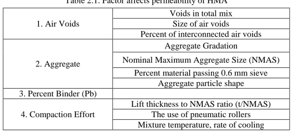
2.1 FACTOR AFFECTING HMA PERMEABILITY ... 15
2.2 STATE OF THE ART – TRADITIONAL APPROACH ... 23
2.3 STATE OF THE ART – PERMEABILITY MODELS ... 32
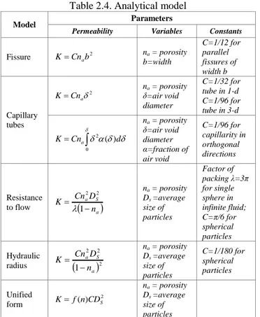
2.3.1 ANALYTICAL MODELS ... 33
2.3.2 PROBABILISTIC MODELS ... 41
2.3.3 NUMERICAL MODELS ... 43
2.3.4 MORPHOLOGICAL ANALYSIS MODELS ... 49
REFERENCES ... 63
3. NUMERICAL GENERATION OF THE MICROSTRUCTURE ... 75
3.1 RSA ALGORITHM ... 76
3.2 CIRCULAR SHAPE OF THE GRAINS ... 80
3.3 ELLIPTICAL SHAPE OF THE GRAINS ... 97
3.4 THE COMPACTION PROCEDURE ... 120
3.5 MONTE CARLO PROCEDURE ... 124
REFERENCES ... 127
4.1 LATTICE BOLTZMANN METHOD IN MODELING FLUID FLOW ... 129
4.2 STEPS OF THE LATTICE BOLTZMANN ALGORITHM ... 137
4.3 UNSTEADY FLOW SIMULATION OF WATER ... 143
4.4 STEADY FLOW SIMULATION OF WATER ... 152
REFERENCES ... 163
5. MODEL VALIDATION ... 166
5.1 EXPERIMENTAL TEST ... 166
5.2 SIMULATION RESULTS: UNSTEADY FLOW SIMULATION ... 171
5.3 SIMULATION RESULTS: STEADY FLOW SIMULATION ... 178
5.4 AGGREGATE SIZE DISTRIBUTION AND HYDRAULIC PERMEABILITY ... 186
REFERENCES ... 189
6. ACOUSTIC CHARACTERISTICS OF OPEN GRADED PAVEMENTS .. 190
6.1 TIRE PAVEMENT NOISE ... 190
6.2 DETERMINATION OF SOUND ABSORPTION COEFFICIENT ... 200
6.3 FIRST EXPERIMENTATION ... 204
6.4 FRACTAL GEOMETRY AND DIMENSION ... 212
6.5 SECOND EXPERIMENTATION ... 220
REFERENCES ... 231
7. CONCLUSIONS AND RECOMMENDATIONS... 234
7.1 CONCLUSIONS ... 234
7.2 RECOMMENDATIONS ... 239
ABOUT THE AUTHOR ... 240
LIST OF FIGURES
1.1 Pavement damage: (a) bleeding; (b) rutting. 3
1.2 Pavement distress: (a) early stages; (b) advanced stages. 3
1.3 Pavement distress - raveling: (a) early stages; (b) advanced
stages. 3
1.4 Pavement distress – localized failures. 3
1.5 Actual design of mix of open-graded pavement. 9
2.1 Darcy’s apparatus. 16
2.2 Schematic curve relating hydraulic gradient and velocity. 17
2.3 Typical Laboratory Regression Line for Permeability
(Choubane et al., 1998). 19
2.4 Internal Voids Structure for Coarse-Graded and
Fine-Graded Mixes (Cooley et al., 2003). 20
2.5 Best Fit Curves for Air Voids versus Permeability for
Different NMAS (Mallick and Cooley, 2003). 20
2.6 Comparison of Permeability at Different Percent Binder
(Giompalo, 2010). 21
2.7 Relationship between Permeability and t/NMAS (Brown et
al., 2004). 22
2.8 Constant Head Permeability Device (Maupin, 2000). 24
2.9 Karol-Warner Falling Head Permeability Device (Daniel et
2.10 NCAT Permeameter by Gilson Company. Inc., Model
AP-1B. 27
2.11 Kuss Field Permeameter (a); Schematic of Kuss Field
Permeameter (b) (Williams, 2006). 29
2.12 Kentucky AIP (Williams et al., 2006). 30
2.13 Schematic of Romus Permeameter (Retzer, 2008). 31
2.14 Some details of hydraulic permeameter (Benedetto et al., 2007).
32
2.15 Different values of porosity in a medium correlated to
hydraulic interconnection among voids. 41
2.16 Nonlinear model of a neuron (Haykin, 2009). 48
2.17 Simulation of HMA mix (Sepehr et al., 1994). 50
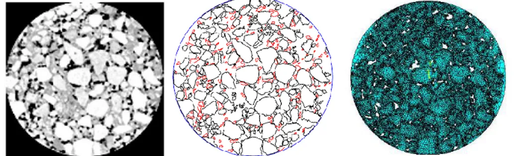
2.18 CT image of an asphalt mixture; CAD image of a polygon model; Digital model after self-adapting meshing (Masad et
al. 2001). 51
2.19 Asphalt modelling concept (Sadd et al., 2003). 52
2.20 The asphalt mixture image and the three-node triangle FEM meshes for the aggregate and mastic subdomains. (a) A scanned image of the specimen surface, (b) The finite element meshes of the specimen surface, (c) Enlarged
meshes for the aggregates and mastic (Dai and You 2007). 54
2.21 Results of Ball model (Cundall and Strack, 1970). 56
2.22 Example to illustrate the AC model particle generation (a) mastic particles in blue, (b) aggregate particles in red, and
(c) AC PFC2D mixture model. 57
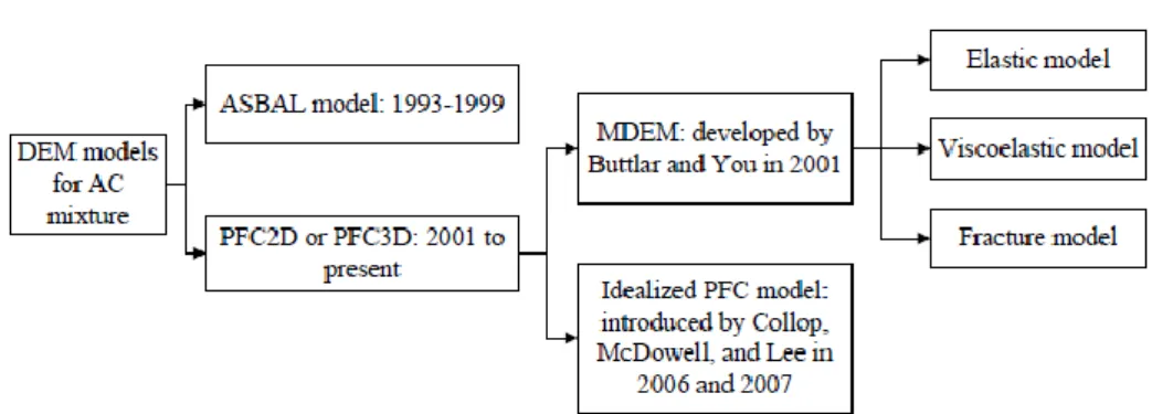
2.24 Summary of DEM models for simulating AC mixtures. 61
3.1 Jamming limit versus aspect ratio. 78
3.2 RSA Algorithm. 79
3.3 Tangency model. 81
3.4 No overlap model. 81
3.5 An example of a grading curve. 83
3.6 Volumes of the grains vs diameters (3d model). 83
3.7 Areas of the grains vs diameters (2d model). 84
3.8 Probability of the choice of grains (3d model). 84
3.9 Probability of the choice of grains (2d model). 84
3.10 Iterative process for the model of bitumen. 89
3.11 Checking the no overlap (2d model). 90
3.12 Checking the no overlap (3d model). 90
3.13 Checking the belonging to the domain (2d model). 91
3.14 Checking the belonging to the domain (3d model). 92
3.15 Architecture of the process. 93
3.16 Extract of output file (Input data). 94
3.17 Extract of output file (coordinates of the inserted particles). 94
3.18 Extract of output file (two-dimensional model). 95
3.19 Extract of output file (three-dimensional model). 95
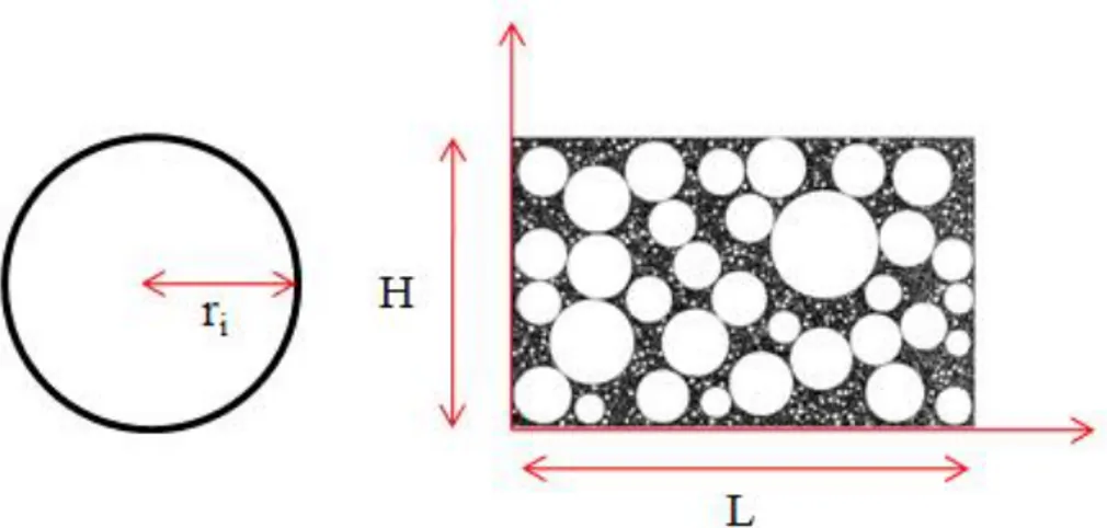
3.21 Ellipse model of the grain. 98
3.22 Matrix model. 99
3.23 The boundary problem. 101
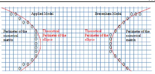
3.24 Approximation of the ellipse. 101
3.25 Area of the three circles. 102
3.26 Area of the ellipse. 102
3.27 Approximation of the ellipse with three tangent circles. 102
3.28 Analytical model. 104
3.29 General equation of the ellipse. 107
3.30 Normal equation of the ellipse. 107
3.31 P-coordinates in a normal ellipse and roto-translate ellipse. 107
3.32 New reference system. 108
3.33 Centered and aligned of the second ellipse to the first. 109
3.34 Solutions of the fourth order polynomial. 111
3.35 Study of the sign of the fourth order polynomial. 112
3.36 Possible conditions for the complex solutions of the
polynomial. 113
3.37 Belonging to another ellipse. 113
3.38 Flow chart of the algorithm. 115
3.39 The model of the thickness of bitumen layer. 116
3.41 Grain’s area and bitumen’s area. 118
3.42 Output on the distribution of grains (txt file). 119
3.43 Output indicators of numerical simulation (txt file). 119
3.44 Visualization of numerical sample. 120
3.45 Marshall compactor. 121
3.46 Superpave gyratory compactor. 122
3.47 Marshall compaction. 123
3.48 Superpave gyratory compaction. 124
3.49 Monte Carlo procedure. 126
4.1 Coalescence between two droplets. 130
4.2 Droplet formation. 131
4.3 (a) Binary image of aggregates, white area representing
aggregates and black area representing the pores, (b)
creation of lattice nodes at the center of each white pixel. 131
4.4 Top-down versus bottom-up approach in fluid flow
simulation. 132
4.5 DxQy lattice microscopic velocity directions. 133
4.6 Flow chart of LB algorithm implemented in this study. 137
4.7 (a) Orientation of components of equilibrium distribution
function calculated in the previous time step, (b) illustration of nonequilibrium distribution function calculated in Step II. 139
4.8 No-slip boundary conditions; half-way bounce back, and
unknown components of the distribution function streaming
4.9 The Lattice in the unsteady flow simulation model. 144
4.10 The Lattice in the unsteady flow simulation model. 145
4.11 The geometry of the numerical sample in the simulation of
the unsteady flow of water. 147
4.12 The first and the last simulation step of the model of the
unsteady flow of water. 148
4.13 The velocity of the particles at the first and the last
simulation step. 149
4.14 Predicted versus measured K-values for different soils. 151
4.15 Track of bands (a) and measure of the length (b) of most
probable water paths (unsteady flow of water). 152
4.16 Extract of the output file of the steady simulation of fluid
flow. 159
4.17 The geometry of the reference domain in the steady
simulation of fluid flow (MATLAB). 159
4.18 The first and the last simulation step of the model of the
steady flow of water. 160
4.19 Δρ during the simulation step. 161
5.1 Permeability test equipment – cross section of pipe. 149
5.2 Permeability test equipment – frontal and lateral view. 149
5.3 Hydraulic transient to saturation – K versus time [s]. 150
5.4 Test of repeatability K versus hydraulic load [10-2 m] two
measurements. 150
5.5 Simulation steps to define the flow paths (step 0 – step 50 –
step 20000) – circular shape of the grains.
5.6 Laboratory results (K – measured) versus theoretical
permeability (K – predicted) – circular shape of the grains. 154
5.7 Simulation steps to define the flow paths (step 0 – step 1000
– step 10000 – step 100000 – step 500000 – step 1000000)
–elliptical shape of the grains. 155
5.8 The last simulation step – elliptical shape of the grains. 156
5.9 Simulation of the water path for the calculation of tortuosity
– elliptical shape of the grains. 156
5.10 Laboratory results (K – measured) versus theoretical permeability (K – predicted) – circular and elliptical shape
of the grains. 157
5.11 Simulation steps in the steady flow simulation model. 159
5.12 Deviations with experimental data (Mix A – 5%). 162
5.13 Deviations with experimental data (Mix A – 5.5%). 162
5.14 Deviations with experimental data (Mix A – 6%). 163
5.15 Deviations with experimental data (Mix B – 5%). 163
5.16 Deviations with experimental data (Mix B – 5.5%). 164
5.17 Deviations with experimental data (Mix B – 6%). 164
5.18 Measured permeability vs predicted values. 165
5.19 Grading area. 166
5.20 K – D50 Regression. 168
6.1 Contributions of the various sub-sources of highway traffic
noise (Donovan, in press) 191
6.2 Vibration caused by tread block/pavement impact 192
6.3 Air pumping at the exit of the contact patch 192
6.4 Air pumping at the entrance of the contact patch 193
6.5 Slip-stick motion of the tread block on pavement 193
6.6 Adhesion between the tread block and pavement at the exit
of the contact patch 194
6.7 The horn effect created by the tire and pavement 194
6.8 Sound amplification caused by organ pipe and Helmholtz
resonator geometries within the contact path 195
6.9 Vibration of the tire carcass around the tread band and at
the sidewall of the contact patch 196
6.10 Acoustic resonance in the air space inside the tire 196
6.11 Exterior noise test results for Wisconsin pavement surfaces
(Kuemmel et al., 2000) 197
6.12 Systematic of acoustically relevant civil engineering
properties of road pavements 198
6.13 Characteristics and parameters that help to describe the
acoustical properties of road pavements 199
6.14 Stationary wave device - Kundt's tube. 200
6.15 Scheme of the Kundt's tube. 201
6.16 Selected grading curves for first experimentation. 204
6.18 Absorption coefficient (α) versus voids content. 206
6.19 Graphical and conceptual framework of the indicators. 208
6.20 I15 versus voids content. 208
6.21 I15 versus absorption coefficient (α). 209
6.22 Conceptual model to explain the increasing dispersion of
data. 210
6.23 Voids content versus absorption coefficient (α). 210
6.24 I15 versus α for each grading curve. 211
6.25 Cantor bar. 213
6.26 Koch curve. 213
6.27 Menger sponge. 214
6.28 Grain dimensions. 216
6.29 Determination of the fractal dimensions for the real mixes. 219
6.30 ω vs fractal dimensions. 219
6.31 α0 vs fractal dimensions. 220
6.32 Selected grading curves for second experimentation. 221
6.33 Average values of absorption coefficient for difference
frequency of measurement. 222
6.34 Noise spectrum for different HMA gradations. 223
6.35 An example of simulation model (chapter 3). 225
6.36 Decreasing trend of the percentage as the number of
6.37 Fractal dimension calculated for the grading curve PA5 at
the time Ndes. 226
6.38 Absorption coefficient versus fractal dimension (200 Hz). 228
LIST OF TABLES
2.1 Factor affects permeability of HMA. 19
2.2 Effect of sawing on permeability (Maupin, 2000). 21
2.3 Advantages and disadvantages of NCATWP and AIP. 27
2.4 Analytical model. 34
2.5 Empirical or Semi-analytical Kmodel. 40
2.6 Summary of the models for rebuilding AC microstructures. 62
3.1 Power law exponents and saturation coverage. 79
4.1 Properties of various LB models. 136
4.2 Relations for the unknowns at the boundaries for D2Q9
model. 142
5.1 Distributions of aggregates dimensions for A and B mixes
(Benedetto, 2007). 167
5.2 Average values of the main physical characteristics of
samples for A and B mixes. 168
5.3 Average values and standard deviations of the measured
permeability for A and B mixes. 171
5.4 Average values and standard deviations of tortuosity for A
and B mixes. 173
5.5 Values of parameters of Walsh and Brace equation from the
output of numerical generation of the asphalt mix sample. 173
5.6 Predicted average values and standard deviations of
5.7 Average values and standard deviations of tortuosity –
elliptical shape of the grains. 175
5.8 Average values and standard deviations of permeability –
elliptical shape of the grains. 177
5.9 Compaction rate obtained by different methods. 178
5.10 Predicted average values and standard deviations of permeability for A and B mixes in the steady flow simulation
model. 180
5.11 Predicted average values of permeability. 180
5.12 Predicted permeability for empirical equations. 181
5.13 Gradings of the samples. 187
5.14 Tortuosity and permeability vs D50. 187
6.1 Noise reduction of different road pavements. 197
6.2 Examples for various types of road pavements. 198
6.3 The absorption values determined through the Kundt’s tube. 205
6.4 The indicators extracted from simulated samples. 207
6.5 Fractal dimensions of grading curves. 219
6.6 Gradations of HMA surfaces teste (Hanson et al., 2004). 223
6.7 Absorption Coefficient α (200 Hz). 224
6.8 Absorption Coefficient α (600 Hz). 224
LIST OF SYMBOLS
The following list shows the key symbols used in the Chapters of this thesis.
a(A), b(B) Semi-major and semi-minor axis of the ellipse A Cross-sectional area of specimen
Ad Area of the domain
Afr Area of the inserted sieve fraction Aifr Limit area of the analyzed size fraction Atotb Total area of bitumen in the sample Atotg Total area occupied by particles b Bitumen content
BF Body force per unit mass of Lattice-Boltzmann equation cS Lattice speed of sound
C Sorting coefficient
Cr Random number
Cs Shape factor of probability models de Effective size of grain
d10 Diameter of grain such that 10 percent of the material is of smaller grains and 90 percent is of larger grains)
D Selected diameter
Dmax Maximum diameter of the reference sieve fraction Ds Average size of the particles
DSy Dimensionless system
DxQy Number of dimensions and number of microscopic velocity directions in Lattice-Boltzmann model
D30 Grain diameter at 30% passing of the reference grading curve D50 Grain diameter at 50% passing of the reference grading curve E* Dynamic axial modulus
fr Fractal dimension
F Distribution function of Lattice-Boltzmann equation g Gravitational acceleration
Gi Distribution of the characteristic dimensions of the grains G* Dynamic shear modulus
hi height of the bitumen film around the grain i-th h1 Initial head of water
h2 Final head of water
Hd Height of the three dimensional domain H12 Transfer function
i Hydraulic or pressure gradient K Permeability coefficient L Length of the specimen
M Number of total particles n Porosity of the porous medium Nc Cumulated number of the elements
Ndes Number of gyration at the initial mixture compaction Nint Number of gyration at the half of the service life Nmax Number of gyration at the end of the service life pˆI Magnitudes of the incident wave
pˆR Magnitudes of the reflecting wave P Physical system
Pb Percent of binder
Pg Compaction rate of grains Psb Specific density of the bitumen
Psg Bulk specific density of the generic particle Ptfr Retained percentage of the analyzed size fraction
Q Flow rate
R Reflection coefficient Rd Radius of the domain Re* Reynolds number
Re’ Modified Reynolds number
Ri Radius of the ith grain belonging to that sieve fraction Sc Particle surface
Sv Specific surface area t Interval of time
T Tortuosity
u Velocity of the fluid uref Reference velocity U0 Superficial velocity Vd Volume of the domain
Vfr Volume of the inserted sieve fraction VIfr Limit volume of the analyzed size fraction Vtotb Total volume of bitumen in the sample Vtotg Total volume occupied by particles
wi Weight factor of Lattice-Boltzmann equation ZS Surface impedance of the material
Z0 Acoustical characteristic impedance of air α Absorption coefficient
αr Aspect ratios
γ Unit weight of the fluid γb Bitumen bulk specific density δx and δt Discrete variables
ε Shape coefficient of the ellipse
θ Jamming limit
v Kinematic viscosity of the fluid ρ Fluid density
τ Relaxation time
τf Cohesion force per area unit
Ω( f ) Collision function of Lattice-Boltzmann equation ∇p Pressure gradient
List of Acronyms and Abbreviations
The following list shows the acronyms and abbreviations used in the Chapters of this thesis.
2-D Two dimensional 3-D Three dimensional AC Asphalt Concrete
AIP Air Induced Permeameter ANN Artificial Neural Network ASF Available surface function CAD Computer Aided Design CFD Computational Fluid Dynamics DEM Discrete element modeling DSR Dynamic Shear Rheometer
FDOT Florida Department of Transportation FEM Finite element modeling
HMA Hot mix asphalt HRA Hot rolled asphalt
KSHFP Kuss Constant Head Field Permeameter LB Lattice Boltzmann
MVR Multivariate Regression
NCAT National Center for Asphalt Technology Permeameter NMAS Nominal maximum aggregate size
PFC Particle Flow Codes PSP Pore size permeameter PVC Polyvinyl Chloride RAP Romus Air Permeameter RMSE Root mean square error RSA Random Sequential Adsorption SGC Superpave Gyratory Compactor SHRP Strategic Highway Research Program SMA Stone matrix asphalt
TLU Threshold Logic Unit UC Unit cell
VDOT Virginia Department of Transportation VTM Percent air voids
1. Introduction
Hot mix asphalt (HMA) is a porous material that has three components: asphalt, aggregates, and air voids. One of the primary factors controlling pavement performance is the ability of HMA to prevent water from remaining within the pavement system.
Moisture related damage in asphalt pavements, that consists in the loss of strength and durability in HMA caused by the presence of water, is global concern.
This kind of damage can be caused by two different mechanisms: adhesive and cohesive failure. Adhesive failures occur when the asphalt binder separates from the aggregate, typically in the presence of water. Cohesive failures occur because of a weakening within the asphalt binder film coating the aggregate, generally owing to moisture effects.
The literature describes five primary mechanisms that lead to either of these failure modes: detachment, displacement, pore pressures, hydraulic scouring, and spontaneous emulsification (Kiggundu, 1988; Asphalt Institute, 1981).
Detachment is described by a microscopic separation of the asphalt film from the aggregate by a thin layer of water without any obvious breaks in the film (Asphalt Institute, 1981; Majidzadeh, 1968; Taylor, 1983). Detachment is believed to be caused by incomplete drying of the aggregate during plant production. Excessive moisture not removed from the aggregate can later migrate within the interstitial pores of an aggregate and lead to detachment of the asphalt film.
Displacement is described as the preferential removal of the asphalt film from the aggregate surface by water (Kiggundu, 1988; Asphalt Institute, 1981; Majidzadeh, 1968). This occurs when water is absorbed into an aggregate through a break in the asphalt film, owing to incomplete coating of the aggregate, rupture of the asphalt film, or loss of dust coatings around the aggregates. Rupture of the asphalt film can occur as a result of fracturing of the aggregates during field compaction, in-service traffic, or environmental action such as freeze–thaw (Kiggundu, 1988). The pore pressure mechanism occurs from the presence of water in the interconnected voids of the HMA (Lottman, 1971). Densification of the HMA under traffic causes the interconnected voids to become isolated (no longer interconnected), and the water is trapped within these isolated
voids. As traffic passes over the HMA, pore pressure increase and then decrease again after the load passes. This continuous increase–decrease of pore pressure can rupture the asphalt film and lead to displacement or hydraulic scour. Hydraulic scour occurs in surface mixes from the application of vehicle tires on a saturated HMA (Kiggundu, 1988; Asphalt Institute, 1981). Water is compressed into the pavement in front of the tire, resulting in a compressive stress within the interconnected void structure. Once the tire passes, a vacuum forms, pulling water back out of the interconnected voids. This compression–tension cycle occurs every time a vehicle passes over the pavement and can lead to moisture damage due to displacement or spontaneous emulsification. Spontaneous emulsification occurs when an inverted phase emulsion (water suspended within asphalt) forms within the HMA (Kiggundu, 1988; Asphalt Institute, 1981).
These modes of failure occur in asphalt pavements as the following types of distress:
Bleeding, cracking, and rutting: These distresses are caused by a partial or complete loss of the adhesion bond between the aggregate surface and the asphalt cement. This may be caused by the presence of water in the mix due to poor compaction, inadequately dried or dirty aggregate, poor drainage, and poor aggregate–asphalt chemistry. It is aggravated by the presence of traffic and freeze–thaw cycles and can lead to early bleeding, rutting, or fatigue cracking. Figures 1.1 and 1.2 show some of the various manifestations of this type of moisture-related distress. Raveling: Progressive loss of surface material by weathering or
traffic abrasion, or both, is another manifestation of moisture-related distress. It may be caused by poor compaction, inferior aggregates, low asphalt content, high fines content, or moisture-related damage, and it is aggravated by traffic. Figure 1.3 shows different stages of this type of moisture-related distress.
Localized failures: This type of distress can be the end result of either of the types discussed above. It is progressive and can be due to the loss of adhesion between the binder and the aggregate or the cohesive strength in the mix itself. Figure 1.4 shows this type of distress.
Structural strength reduction: This is a result of a cohesive failure causing a loss in stiffness in the mixture.
(a) (b) Figure 1.1 – Pavement damage: (a) bleeding; (b) rutting.
(a) (b)
Figure 1.2 – Pavement distress: (a) early stages; (b) advanced stages.
(a) (b)
Figure 1.3 – Pavement distress - raveling: (a) early stages; (b) advanced stages.
To prevent these infiltration related distress and to control the fundamental parameters of the mix, in 1993, Superpave (Superior Performing Asphalt Pavement) mix design system was introduced as a part of Strategic Highway Research Program (SHRP). Hot mix asphalt (HMA) pavements have been produced with coarser gradation than previously used mix design methods (open-graded pavement). Open graded pavements are considered potentially to be effective solutions. These asphalt mixes with high degrees of porosity (open-graded mixes) drain significantly better than normal pavement materials presenting a high value of the index of the voids and hydraulic interconnection among them but provide also some disadvantages related to the cost and the maintenance of the pavement.
Advantages and disadvantages of porous asphalt have been well established in the literature (Younger et al., 1994), and they can be summarized as follows.
Advantages - Reduction in splash and spray, reduced aquaplaning: compared to dense mixes, surface water can drain through porous asphalt due to the large amount of continuous pores in the structure. The material provides good visibility under rainy conditions, thus preventing the reduction in traffic flow volumes, which normally accompany rain. In addition, the absorption of surface water is effective in reducing aquaplaning which occurs when vehicles move at high speeds on a thin water layer. It has been shown that porous asphalt contributes to the reduction of the number of accidents in rainy days (Maupin, 1976).
Reduction in light reflection and headlight glare: because porous asphalt
acts as a drainage layer, enabling rainwater to percolate through the mix, thus light reflection and headlight glare, some of the dangerous factors for drivers especially in night time, decrease dramatically and lane markings are enhanced clearly on wet surfaces.
Improvement in Skid Resistance, Reduction in vehicle rolling resistance:
increasing skid resistance under wet conditions is one of the main reasons for using porous asphalt. Assuming that a rougher wearing course would increase frictional properties. In Oregon friction properties of porous asphalt were compared with dense graded asphalt. The data accumulated indicated that porous asphalt mixes had slightly improved friction properties in dry conditions and a much improved friction properties during rainy conditions when free water was present on the pavement (Moore et al., 2001). Skid resistance is a function of macro and micro textures. At high speeds, the contribution of the macro texture is more
dominant. In the A38 Burton trial section, 1987, Porous asphalt showed a skid resistance at least as good as that of the HRA (hot rolled asphalt) (Daines, 1992). In Japan, it is reported that the skid resistance of porous asphalt was initially the same as conventional nonporous asphalt, but this value increased gradually during the service life, whereas the dense mixes did not show any significant change. In addition, fresh porous asphalt layers may have a reduced skid resistance due to the bitumen film on the aggregates exposed to the surface. It is noteworthy to mention that some Swiss experts recommend not using porous asphalt with aggregate size in excess of 16 mm on wearing courses. According to their experience, the use of larger top size aggregates may provide less skid resistance on wet road surfaces.
Rut-resistance: in Japan, despite its high porosity, a number of trial
sections show lower permanent deformation on porous asphalt than other dense mixes. Tighter aggregate skeleton in porous asphalt may contribute to withstand the load under traffic (EHRFJ, 1993). On the 1987 Burton trial in the UK, the deformation rate of this porous asphalt section in the near side lanes was less than 2 mm/year and 0.5 mm/year on average after 8 years trafficking. This result was evaluated as an acceptable rate in Britain. Although deformation of pavement depends on several conditions, such as climate, traffic intensity and loads, porous asphalt may provide acceptable rut resistance compared to other dense mixes (Daines, 1992).
Noise Reduction: road surfaces are laid with coarse macro-texture, which
are in contact with the tire tread. This texture is known to contribute to the noise absorption between the surface and the tire. Many trial sections show lower noise levels on porous asphalt, which may be 6 dB(A) lower than concrete layers (Tesoriere et al., 1989) or 2 to 6 dB(A) lower than the HRA (Nicholls, 1996). According to the Swiss standards, under dry conditions in a 70 dB(A) area by using porous asphalt a noise reduction of 5 dB(A) can be achieved (SN 640 433b, 2001). Swiss experience also indicates an advantage on the high speed traffic lanes in excess of about 80 km/h. Although the noise level of porous asphalt on the lower speed lanes is almost the same as other conventional dense mixes, porous asphalt is still effective in reducing the noise in the frequency range of 1.25 to 2 kHz at 60 km/h (Köster, 1991). The experience in the Netherlands indicates that on the lower traffic speed lanes less than 70 km, the noise level of porous asphalt is even higher than dense mixes due to its rough macro-texture on the surface. To improve this aspect, 2 layer
porous asphalt (twinlay) was developed (Bochove, 1996). It consists of a bottom layer of the porous asphalt with a coarse single grained aggregate (11/16 mm) and a thin top layer of fine graded porous asphalt (4/8 mm).This double-layer structure can contribute to reduce the traffic noise at any vehicular speed. According to their report, additional advantages of the twinlay are better clog resistance against dirt and better cleaning properties. Therefore, this unique structure is expected to be introduced in their urban areas on a regular basis to meet the high environmental demand. Japanese experience reveals that porous asphalt is effective in noise reduction, but that this advantage is gradually lost over the years due to a decrease in mix porosity, especially in snowy areas where tire chains are used (JHPC, 1994). As an example from the USA in Oregon, two types of noise measurements were taken. The first was roadside noise and the second was interior vehicle noise. The results indicated that porous asphalt pavements reduce the noise in the higher-frequency zones. This conclusion is supported mostly from the roadside measurements and not from those taken in the interior of the vehicle, possibly since the higher frequencies are dampened by the vehicle
Disadvantages - Aging and Ravelling: although porous asphalt has many obvious advantages, there are also some disadvantages. One of the most critical factors in the performance of bituminous mixes is the tendency of the binder film on the surface of the aggregate to be continuously exposed to oxygen, sunlight, water etc. This results in binder hardening and a reduction in pavement service life (Hoban et al., 1985). When bitumen hardens, aggregates can be stripped easily from the asphalt mixes. It is well known that, due to its high porosity, porous asphalt ages much faster than conventional dense mixes. In full-scale road trials in the UK, the results conclude that the life of porous asphalt is ultimately limited by binder hardening with likely failure when its penetration drops below 15 pen (Daines, 1992).Another potential disadvantage of porous asphalt is the water sensitivity of the mix. Rainwater can penetrate through the porous matrix. Sometimes the water remains in the structure keeping the asphalt in wet condition for a long time. This moisture can cause some extra damage in porous asphalt by ravelling the binder film from the aggregate surfaces.
Reduction in Porosity: during service life, the pores tend to be clogged by
dirt, dust or other clogging agents. On high speed lanes, tires produce a self-cleaning effect (Van Heystraeten et al., 1990). Thus clogging is more serious on low speed lanes or minor roads. With the loss of pores, the
advantages of noise reduction and drainage function will gradually disappear. This is another serious problem for road maintenance. To overcome this disadvantage many types of cleaning methods, including vacuum vehicles with hydraulic jet water, have been developed to maintain the advantage of porous asphalt long term. However, no conclusion on the optimum type of cleaning method can be recommended. Porosity loss is also caused by secondary traffic compaction, especially on heavy routes.
Shorter Service Life: due to the above listed disadvantages, the service life
of porous asphalt surfaces is shorter than that of dense mix layers. In addition, it depends on several factors such as binder content and type, aggregate gradation, traffic volume and climate. Although previous experiences show an optimistic life expectancy of around 15 years, some maintenance should be necessary within about 5 to 8 years according to the results in many countries. Such maintenance costs for porous asphalt (from cleaning the clogged pores to replacement of those layers, which lost their drainage function) are considered higher than for the conventional asphalt. However, this does not mean that cost-effectiveness of porous asphalt surface is lower than that of other surface mixes. When this issue is discussed, the significant contribution of this pervious layer for social benefits, such as traffic safety and environmental issues, can not be ignored.
Winter Maintenance: snow and ice removal from porous surfaces requires
at least twice the quantity of de-icing salt treatment compared to that of other dense mixes. However, the damage to porous asphalt due to salt is still unclear. Vehicular tire chains, spiked tires and snow ploughing sometimes cause severe damage on the open textured mixes requiring additional repair when the aggregates are stripped from the surface. Swiss standards recommend explicitly that porous asphalt not be used in areas where chains and spiked tires are used (SN 640 433b, 2001). CEN suggests an abrasion test by studded tires to evaluate the chain damage (EN13108-7, 2006).Japan also applies either a similar test for porous asphalt, which was originally developed for dense mixes in snowy areas, or a decrease in the temperature down to - 20 °C in the Cantabro test (Japan Highway Public Corporation, 1994). It should be noted that, because of the lower thermal conductivity of the porous asphalt, in winter this surface may colder than dense asphalt (Köster, 1991). Therefore, on the porous asphalt surface, snow tends to settle earlier and remain longer, also ice forms earlier when the roads are wet (Nicholls, 1996).
1.1 Problem Statement
All these aspects and several research and applications (Qi et al., 1995; Kandhal and Mallick, 1998) show that one of the most important factor that influence the performance of the open-graded asphalt pavement and its behavior during the service life is the design of the mix, that affects also its durability and its safety. In particular one of the main challenge in designing an open graded pavement is determining a reasonable compromise between mechanical and hydraulic characteristics of open graded mixtures. They depend on the road materials and mix design as on how the pavement is developed. Traditionally a conceptual approach, physically based, is followed to identify materials requirements and construction standards. Conceptual models are generally approximated and, consequently, laboratory tests on the mixes or measurements on the real scale are performed to check the final characteristics of pavement. More in depth, this approach is mostly effective if the design objective is univocal, but if the mixture must respect different and concurrent requirements as mechanical and hydraulic standards the approach is not of great effectiveness (Nukunya et al., 2001). In particular, the case of hydraulic and mechanical properties of mixes is very intriguing because two different objectives are concurrent. In fact an adequate hydraulic permeability is possible if the voids content is high and the voids system is open (Cooley et al., 2003; Masad et al., 2003). On the contrary the mechanical characteristics depend on cohesion and friction among aggregates and low levels of voids content are required. The mix design appears in this case as an optimization problem. However, because there are no analytical nor empirical model available, it often happens that the mixture is designed adopting a minimum standard for mechanical characteristics and the hydraulic permeability is overestimated (figure 1.5). This oversize produces many disadvantages and problems from an economic and environmental point of view (Benedetto et al., 2007). It is very difficult to solve this optimization problem. In fact, while the mechanical properties can be investigated through standardized laboratory measurements, the traditional approach used to evaluate the expected
drainage capability of pavement is controversial. It is based on laboratory tests using hydraulic permeameters (Kanitpong et al., 2001) or measures on the field (Cooley, 2003), and it is unable to reach a correct estimation of permeability due to many approximations in measurements and to the wide variety of devices, described in the following chapter, that work under different conditions and measuring different parameters.
Figure 1.5 – Actual design of mix of open-graded pavement
In order to solve these problems in the last decades several researchers have attempted to calculate permeability of porous media through analytical model, by determining correlations with some fundamental parameters of the mix. These correlations, however, because not considering all the factors, are not able to define a univocal process, causing uncertainty and approximation of prediction. For this reason, recently, in order to determine the performance of HMA mixes some studies, based on numerical simulations at the micro-structural levels, have been carried out (Masad et al., 2000, Al Omari et al., 2002), as shown in the following chapter. These models return reliable values of permeability but require expensive and onerous experimental procedures for the knowledge of the internal microstructure.
In this study, considering these approaches, we propose a novel simulation approach based on different algorithms, written in C++ language, in order to predict the properties of an open-graded asphalt pavement during its service life. These novel approaches reduce computational complexity of the simulation models and increase the reliability of empirical methods, described in the following chapter. More in depth the proposed methods integrate different numerical models. These models allow to determine:
1) physical characteristics, through generation of the physical micro - structure of the mixture from the design inputs using RSA algorithm;
2) hydraulic properties, by the simulation of flow of water within the numerical sample, based on the Lattice– Boltzmann method (LB) (Montessori et al., 2014);
3) acoustic performance, by the creation of a new experimentation and by the definition of additional variables.
The new procedures are validated comparing the results of numerical simulations with the experimental data and analytical predictions.
1.2 Objectives
The overall objective of this study is to develop a new numerical procedure to predict pavement performance in order to support the design and to optimize the mixture. This procedure is obtained through the numerical simulation, that allows a wide reproducibility of the tests, an ease of manipulation of the phenomena and significant improvements from an environmental and economic point of view.
The specific objectives of this study are summarized as follows:
a) Develop a numerical model for the characterization of the physical microstructure of sample using RSA algorithm;
b) Use different algorithms for the compaction of the samples in order to represent the real conditions adopted in laboratory for the packaging of the mixture, according to the standards of Marshall test and Superpave gyratory method;
c) Develop numerical models for the simulation of fluid flow (steady and unsteady) in the synthetical microstructure of asphalt mixes; d) Calculate the drainage capability of the simulated open-graded
asphalt samples using the developed numerical models;
e) Validate the developed models through comparing their results to HMA measurements and empirical predictions;
f) Determination of acoustic performance at different time of the service life of the pavement using a new measuring device;
g) Predict the acoustic properties starting from the grain size distribution through the characterization of the microstructure of the samples.
1.3 Dissertation Outline
The dissertation consists of seven chapters. In Chapter 1, an introduction to the dissertation is presented. The introduction includes the problem statement, the specific objectives of the research, and the dissertation outline.
Chapter 2 describes the literature review that is relevant to the subject. Factors affecting permeability of porous materials are discussed. The different experimental methods for measuring permeability of HMA in the field or in the laboratory are reviewed. Permeability models including the analytical, probabilistic, and numerical models are also presented. Empirical models, based on analytical equations, are showed.
Chapter 3 describes the algorithms used for the numerical generation of the microstructure of samples of open-graded pavement. The compactions methods that are applied to synthetical samples are also included in this chapter.
Chapter 4 includes the derivation of the numerical model for fluid flow simulation. The development of two different models that simulate the unsteady, in the first approach, and the steady, in the second one, fluid flow are also included.
In Chapter 5, the outputs of the numerical model are discussed. These outputs include the permeability values obtained numerically that are compared to measured permeability of HMA mixes and analytical predictions of empirical models.
Chapter 6 describes the measurement of acoustic properties of open-graded asphalt samples. The comparison between these properties and some numerical indicators extracted from the simulated samples is also included in this chapter.
The last chapter, Chapter 7, is the dissertation summary that reviews the main tasks of this study and includes the dissertation conclusions and some recommendations for future work.
References
1. Al-Omari, A., Tashman, L., Masad, E., Cooley, A., and Harman, T. (2002). Proposed Methodology for Predicting HMA Permeability. Journal of Association of Asphalt Paving Tech., 71, 30-57.
2. Asphalt Institute (1981). Cause and Prevention of Stripping in Asphalt Pavements. Educational Series No. 10., College Park, Md..
3. Benedetto, A. (2007). Open graded asphalt mixes: permeability and mechanical characteristics. International Journal of Pavement, 6, 63-74.
4. Bochove, G.G. (1996). Twinlay, a New Concept for Porous Apshalt. Proc. Eurasphalt & Eurobitume Congress.
5. Cooley, L.A.Jr., Mallick, R.B., Teto, M.R., Bradbury, R.L., Peabody, D. (2003). An Evaluation of Factors Affecting Permeability of Superpave Designed Pavements. NCAT Report, 2-3, 29p.
6. Daines, M.E. (1992). Trials of porous asphalt and rolled asphalt on the A38 at Burton, Department of transport TRRL Re-port RR323, Transport and Road research Laboratory, Crowthorne.
7. EN13108-7, (2006). Provisional European Standard, Bituminous mixtures material specifications Part 7- porous asphalt (PA).
8. Express Highway Research Foundation of Japan, (1993). Report of Study and Research for Porous Asphalt. Tokyo.
9. Hoban, T. W. S., Liversedge, F., and Searby, R., (1985). Recent Developments in Pervious Macadam Surfaces. Proc. 3rd Eurobitumen Symp., The Hague, 635-640.
10. Japan Highway Public Corporation, (1994). Design and Execution Manual for Porous Asphalt. Tokyo.
11. Kandhal, P.S. and Mallick, R.B., 1998. Open Graded Friction Course: State of the Practice. NCAT Report, No. 98-7.
12. Kanitpong, K., Benson, C. H., and Bahia, H. U. (2001). Hydraulic conductivity (permeability) of laboratory compacted asphalt mixtures. Transportation Research Record, 1767, 25-33.
13. Kiggundu, B. M., and Roberts F. L. (1988). Stripping in HMA Mixtures: State-of-the-Art and Critical Review of Test Methods.
Report 88-2. National Center for Asphalt Technology. Auburn University, Auburn, Ala.
14. Köster, H., (1991). Observation of the behavior of porous asphalt under traffic. VSS report Nr. 218.
15. Lottman R. (1971). The Moisture Mechanism that causes asphalt stripping in asphalt pavement mixtures. University of Idaho.
16. Majidzadeh, K., and F. N. Brovold (1968). Special Report 98: State of the Art: Effect of Water on Bitumen-Aggregate Mixtures. HRB, National Research Council, Washington, D.C.
17. Masad, E. A., Muhunthan, B., and Martys, N. (2000). Simulation of fluid flow and permeability in cohesionless soils. Water Resources Research, 36(4), 851–864.
18. Masad, E.A., Birgisson, B., Al-Omari, A., Cooley, A. (2003). Analysis of Permeability and Fluid Flow in HMA. Proceedings of the 82nd Transportation Research Board, Washington, DC.
19. Maupin G W., (1976). Virginia‟s Experience with Open-Graded Surface Mix. Transportation research Record, 595, 48-51.
20. Montessori, A, Falcucci, G, Prestininzi, P, La Rocca, M, Succi, S. (2014). Regularized lattice Bhatnagar-Gross-Krook model for two- and three-dimensional cavity flow simulations. Physical Review E, 89, 5.
21. Moore, L.M., Hicks, R.G., and Rogge, D.F., (2001). Design, Construction, and Maintenance Guidelines for Porous Asphalt Pavements. Transportation Research Record 1778.
22. Nicholls J.C., (1996). Review of UK porous asphalt trials. TRL Report 264, Transport Research Laboratory, Crowthorne.
23. Nukunya, B., Roque, R., Tia, M., and Birgisson, B. (2001). Evaluation of VMA and other volumetric properties as criteria for the design and acceptance of Superpave mixtures. Proc. of AAPT, 70, 38-69.
24. Qi, X. and Sebaaly P.E., (1995) Evaluation of Polymer- Modified Asphalt Concrete Mixtures. Journal of Materials in Civil Engineering, 117-124.
25. SN 640 433b., (2001). Drainasphaltschichten, Konzeption An-forderung, Ausführung. Swiss, Standards for porous asphalt Original in German and French.
26. Taylor, M. A., and Khosla N. P. (1983). Stripping of Asphalt Pavements: State of the Art. Transportation Research Record 911, National Research Council, Washington, D.C., 150–158.
27. Tesoriere, G., Canale, S., and Ventura, F. (1989). Analysis of Draining Pavements from a Point of View of Phono-Absorption. Proc. 4th Europian Symp., Madrid, 878-881.
28. Van Heystraeten, G., and Moraux, C. (1990). Ten Years‟ Experience of porous Asphalt in Belgium. Transportation Research Record 1265: 34-40.
29. Younger, K., Partl, M., and Hicks, R.G. (1994). Evaluation of porous pavements for road surfaces. Interim Report, Oregon State University, department of civil engineering, Corvallis.
2. Literature Review
This chapter presents a review of the literature pertinent to the topic of this dissertation on the performance of porous materials with emphasis on open-graded asphalt mixes. The basics that govern the permeability of porous media are discussed first. Then, a review of permeability models (analytical, probabilistic, morphological, and numerical models) is presented.
Permeability measurement devices and empirical methods are presented briefly to develop appreciation of the experimental factors that influence the ability to compare the permeability of different HMA mixes. Finally, recent studies on the permeability of HMA are summarized.
2.1 Factor affecting HMA permeability
Permeability of porous media is defined as the ability to transmit fluids through the voids of the porous material when it is subjected to different hydraulic loads. Hydraulic conductivity is numerically defined by Darcy‟s Law, derived from the Darcy‟s experiments (Figure 2.1), which states that the fluid discharge velocity is directly proportional to the hydraulic gradient (Darcy, 1856). It can also be considered as the flow rate (Q), in units of volume, passing through a cross-sectional area of the porous medium in unit time, under the influence of a pressure gradient (i). Darcy‟s law depends on the flow condition and it is expressed in the following form:
KiA
Q (2.1)
where, K is the proportional factor called hydraulic conductivity (or permeability coefficient), Q is the flow rate in unit of volume, A is the
cross-sectional area, i is the hydraulic or pressure gradient, defined as the pressure difference (Δh) divided by the length of the hydraulic path (L).
Figure 2.1. Darcy‟s apparatus
The flow rate divided by the cross-sectional area represents the average velocity of the fluid flow (v). Permeability coefficient (K) is expressed in velocity units for a given hydraulic head.
Darcy‟s law, applied to a porous medium, is valid when the fluid travels at a very low speed and no turbulence occurs. More in depth the classification of fluid flow into steady, transient, or turbulent flow depending on the variability of flow velocity in time or direction. Fluid flow in porous media is driven by two different mechanisms. The first one is known as the creeping flow, which is due to the fluid viscosity. The second one is convection flow, which is due to the inertial forces. The significance of either one of these terms depends on the value of the modified Reynolds number (Re*), which combines fluid density (ρ), viscosity (μ), velocity of flow (v), and a characteristic dimension of the particles of porous media (D), (Scheidegger 1974). It is expressed in the following form: vD * Re (2.2)
For the same fluid and porous material, the velocity changes as a function of the applied pressure gradient in the direction of the flow as illustrated in figure 2.2. The linear part of the curve represents the region of small Re* where creeping flow is the dominant mechanism.
Since fluid flow in porous materials is considered as laminar flow, then, permeability of most porous materials is usually calculated assuming small Re* in the linear range of the curve shown in figure 2.2. This
assumption has been verified in numerical simulations of fluid flow in the internal structure of porous media such as sandstone, cement paste, and sands (Adler et al. 1990; Martys et al. 1994). Scheidegger (1974), therefore, showed that permeability of porous materials depends on the properties of the porous material and the fluid, following this expression:
k
K (2.3)
where k is a component of the absolute permeability tensor; K is the Darcy‟s permeability coefficient, as defined previously, γ is the unit weight of the fluid and μ is the viscosity of the fluid.
Figure 2.2. Schematic curve relating hydraulic gradient and velocity
It can be seen from Eq. (3) and as reported by Scheidegger (1974) that permeability of porous materials depends on the properties of the porous material and the permeative fluid. The properties of the porous material are presented by the absolute permeability (K) which is a function of the porous material only. The properties of the permeative fluid are presented, on the other hand, by its unit weight and viscosity. As Dullien (1979) pointed out, it is more scientific and more useful to separate the contribution of porous material from that of the permeative fluid.
Since permeability of porous materials depends on the properties of the fluid and those of the porous material, permeability will be affected by any changes in their properties. The viscosity and the unit weight of the permeative fluid are mainly affected by temperature. The porous material,